Integrated approaches to climate–crop modelling: needs and challenges

Abstract

This paper discusses the need for a more integrated approach to modelling changes in climate and crops, and some of the challenges posed by this. While changes in atmospheric composition are expected to exert an increasing radiative forcing of climate change leading to further warming of global mean temperatures and shifts in precipitation patterns, these are not the only climatic processes which may influence crop production. Changes in the physical characteristics of the land cover may also affect climate; these may arise directly from land use activities and may also result from the large-scale responses of crops to seasonal, interannual and decadal changes in the atmospheric state. Climate models used to drive crop models may, therefore, need to consider changes in the land surface, either as imposed boundary conditions or as feedbacks from an interactive climate–vegetation model. Crops may also respond directly to changes in atmospheric composition, such as the concentrations of carbon dioxide (CO₂), ozone (O₃) and compounds of sulphur and nitrogen, so crop models should consider these processes as well as climate change. Changes in these, and the responses of the crops, may be intimately linked with meteorological processes so crop and climate models should consider synergies between climate and atmospheric chemistry. Some crop responses may occur at scales too small to significantly influence meteorology, so may not need to be included as feedbacks within climate models. However, the volume of data required to drive the appropriate crop models may be very large, especially if short-time-scale variability is important. Implementation of crop models within climate models would minimize the need to transfer large quantities of data between separate modelling systems. It should also be noted that crop responses to climate change may interact with other impacts of climate change, such as hydrological changes. For example, the availability of water for irrigation may be affected by changes in runoff as a direct consequence of climate change, and may also be affected by climate-related changes in demand for water for other uses. It is, therefore, necessary to consider the interactions between the responses of several impacts sectors to climate change. Overall, there is a strong case for a much closer coupling between models of climate, crops and hydrology, but this in itself poses challenges arising from issues of scale and errors in the models. A strategy is proposed whereby the pursuit of a fully coupled climate–chemistry–crop–hydrology model is paralleled by continued use of separate climate and land surface models but with a focus on consistency between the models.

1. Introduction

In modelling studies of climate change and its impacts, including impacts on crop production, the climate system is typically represented as a number of sub-systems such as the atmosphere, croplands, natural ecosystems and hydrology. The interactions between these sub-systems can be treated with two different methods. The traditional, disciplinary method is to assume a linear cause–effect chain in which one sub-system is simulated first, and the resulting state is then applied as input to a second sub-system model, and so on. For example, projections of radiatively forced climate change and its impacts on crops, generally, consist of such a linear sequence of simulations with models of different components of the climate system. Scenarios of greenhouse gas and aerosol emissions are derived with models, which follow scenarios of future changes in population, technology and economic state. These emissions scenarios are then translated into scenarios of greenhouse gas concentrations in the atmosphere, using models which consider the processes acting to reduce concentrations either by chemical processes in the atmosphere or uptake at the land and ocean surfaces. These scenarios of greenhouse gas rise are then applied as inputs to climate models such as General Circulation Models (GCMs), which compute the radiative forcing due to the greenhouse gas rise and the consequent changes in climate. The resulting climate scenarios are then applied to further models, which simulate the response of crops (Gitay et al. 2001).

The scenarios of future climate change simulated with global GCMs and Regional Climate Models (RCMs) are typically applied only to the issue of radiatively forced climate change, in order to provide general assessments of climate change and its impacts in order to assess the need for limiting fossil fuel emissions. These models, generally, focus on processes that are important for large-scale climate. However, planning for adaptations to climate change such as changes in farming systems will require information on specific local climate changes. Although, this need is partly addressed through the use of RCMs, which provide finer-scale climate change simulations and better resolve regional-scale processes such as orographic effects, the current generation of RCM simulations only consider the responses to large-scale radiative forcings. Local climatic drivers such as human-induced landscape and water budget changes and the physiological responses of vegetation to carbon dioxide (CO₂) rises are not routinely considered. The models also neglect climatically induced landscape changes, which may provide feedbacks on local climate change. These landscape, water budget and plant physiological changes may all be affected by crop-related processes. If these simulations are used to inform studies of the impacts of climate change on food crops, the local climate changes may, therefore, be inconsistent with the nature of cropland which would be associated with the climate change. The resulting predictions of crop production may therefore be unrealistic. Sections 2 and 3 of this paper discuss the potential implications of these omissions.

Croplands may also play a role in large-scale climate feedbacks. Simulations with coupled climate–carbon cycle models have suggested the potential for significant feedbacks on climate change involving the terrestrial carbon cycle and methane emissions from wetlands. Since, a large proportion of the global land surface consists of croplands and paddy rice makes significant contribution to methane emissions from wetlands, the strength of the global feedbacks on climate change from carbon dioxide and methane fluxes may depend on crop-related processes. These are discussed in §4.

Another issue which requires consideration is the direct effects of changes in atmospheric composition on crops, for example, through CO₂ fertilization or Ozone (O₃) damage, in addition to the indirect effects of these atmospheric constituents on climate through radiative forcing. It may also be necessary to consider the interaction between food crops and other impacts sectors. For example, if crop properties modify the surface water budget, the hydrological responses to climate change may be modified by the responses of crops. Furthermore, crop management activities such as irrigation may affect other impacts sectors such as water resources or flood risk. The implications of these interactions are discussed in §§5 and 6.

Studies of climate change impacts on crops are also subject to a number of practical difficulties. Although climate models, generally, operate on timesteps of under 1 hour so can produce sub-daily information, this information has been largely under-exploited because the sheer quantity of output data can present technical difficulties in transferring and processing for use as input to impacts models. In some cases, quantities of interest to crop research such as potential evapotranspiration or thermal time could be calculated within GCM land surface schemes, thus saving on data transfer and post-processing, but this is not routinely done because such quantities are not required for the atmospheric model. Furthermore, the sequential approach to performing climate model simulations first followed by impacts model simulations later can mean that a long period of time is required for assessments of the impacts of climate change on crops. This can cause difficulties in presenting a consistent assessment of the latest results in both the climate modelling and crop modelling fields; at any given time, the most recent set of crop model results may well have been driven by output from an older set of climate model results. These issues are discussed in §7.

The above issues could be addressed through the full integration of crop models into climate system models, to make a climate–crop system model in which all relevant forcings, feedbacks and synergisms are considered. However, such integration would itself be not without its difficulties, as will be discussed in §8. This paper concludes with a discussion of the trade-off between the advantages and disadvantages of a fully integrated climate–crop model, and presents recommendations for future progress in simulating climate change impacts on crops.

2. Overlooked forcings of regional climate change

Although, the forcing by increasing greenhouse gas emissions includes a contribution from deforestation, this is only one means by which land cover change can influence climate. Vegetation also influences the surface fluxes of radiation, heat, moisture and momentum, so if the large-scale character of the vegetation cover is modified, changes to the climate can result. Conversion of forest to cropland or pasture can reduce the aerodynamic roughness of the landscape and decrease both the capture of precipitation on the canopy and the root extraction of soil moisture; these changes tend to decrease evaporation and hence the fluxes of moisture and latent heat from the surface to the atmosphere, which act to reduce the return of moisture to the atmosphere for precipitation and increase the temperature near the surface. Also, a forested landscape, generally, has a lower surface albedo than open land, particularly in conditions of lying snow when shortwave radiation is trapped by multiple reflections within the forest canopy (Bonan et al. 1992; Thomas & Rowntree 1992; Harding & Pomeroy 1996). Deforestation can, therefore, lead to increased shortwave reflection, which provides a cooling influence. The relative importance of these processes depends on the local background climatic conditions and can vary with season and location (Betts 1999; Bounoua et al. 2002).

Deforestation of the boreal and temperate forests would, therefore, exert a cooling influence on climate (Douville & Royer 1997), and indeed from the global perspective, most deforestation until the mid-twentieth century occurred in the temperate regions (figure 1). Model results suggest that this has exerted an overall local cooling effect (Brovkin et al. 1999; Betts 2001; Govindasamy et al. 2001) (figure 2). However, in more recent decades, land abandonment in Western Europe and North America is leading to reforestation which would cause a warming influence. This is projected to continue in the temperate regions in most of the scenarios currently considered by the Intergovernmental Panel on Climate Change (IPCC), and in some scenarios reforestation also features in other regions such as China (Watson et al. 2000) (figure 3). Reforestation in temperate regions would be expected to exert a warming influence through decreased surface albedo (Betts 2000).

Figure 1.

Present-day distribution of croplands derived from satellite remote sensing and inventory data (Ramankutty & Foley 1999).

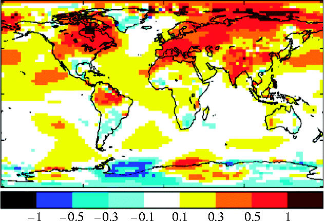
Figure 2.

Effects of historical land cover change on near-surface temperature (K) simulated with the HadAM3 GCM. Difference in temperature (K) between simulations with current vegetation and potential natural vegetation (Betts 2001).

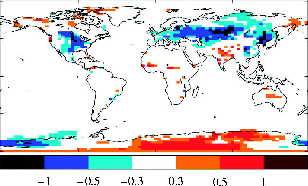
Figure 3.

Two scenarios of fraction of land under agriculture at 2100, consistent with the IPCC Special Report on Emissions Scenarios (Nakićenović et al. 2000). (a) Scenario ‘A1b’ (global population peaks mid-century; very rapid economic growth; more efficient technologies; advancements balanced across energy sources). (b) Scenario ‘A2’ (continuous population growth; fragmented, slower, regionally oriented economic growth). Scenarios from the IMAGE model (Alcamo et al. 1998); data supplied by Detlef van Vuuren, RIVM.

In contrast, the tropical forests are, currently, subject to a rapid rate of deforestation (figure 3), and this would also be expected to exert different influences on climate at both local and global scales. The effects may be different to those resulting from changes in the boreal forests. A large number of modelling studies have examined the climate sensitivity to total deforestation in tropical regions such Amazonia. There is general agreement among these studies that complete deforestation would cause a warming of surface temperature and reduction in precipitation, due to a reduced level of transpiration from the deforested landscape (Lean & Warrilow 1989; Kleidon & Heimann 2000. See Lean & Rowntree (1997) for a summary of several studies). The smaller flux of moisture due to reduced transpiration causes an increase in the ratio of sensible to latent heat fluxes (the Bowen ratio), so the air near the surface is warmed. Since much of the rainfall in the Amazon basin relies on water transported from over the oceans through the repeated cycling of water through rainfall and evaporation (Salati & Vose 1984), the reduced transfer of moisture to the atmosphere also decreases the recycling of moisture across the continent. Less moisture is, therefore, available for precipitation in the centre and west of the Amazon basin. In addition, an increase in surface albedo results in a smaller heating of the surface by the net radiation balance, suppressing ascent and hence causing less moisture to be drawn into the region (Charney 1975). A reduced frictional drag exerted by the deforested landscape will also act to reduce this moisture convergence. All these mechanisms will tend to reduce precipitation (figure 4). Assessments of the impacts of climate change in the tropics should, therefore, also take account of the effects of changes in land cover on climate. Simulations of the impacts of climate change on crop production in both temperate and tropical regions should, therefore, take account of the effects of the associated changes in land cover on climate (Pielke 2002; Pielke et al. 2002).

Figure 4.

Effects of total Amazonian deforestation on precipitation in the South American region (mm d⁻¹) simulated with the 1993 version of the Hadley Centre GCM. Difference in precipitation (mm d⁻¹) between simulations with totally deforestated Amazonia and current forest (Lean & Rowntree 1993).

Irrigation can also increase the surface moisture flux and hence reduce the Bowen ratio, exerting a cooling influence on local near-surface temperatures. Boucher et al. (2004) introduced present-day patterns of irrigation into the LMD GCM and found a simulated surface cooling of up to 0.8 K in some regions (figure 5).

Figure 5.

(a) Present-day water vapour flux from irrigation (kg m⁻² yr⁻¹). Data from Döll & Siebert (2000, 2002) as presented by Boucher et al. (2004). (b) Effect of present-day irrigation on surface temperature (K) in the LMD GCM. Difference in temperature (K) between simulations with and without irrigation. Boucher et al. (2004), copyright Springer-Verlag.

A further anthropogenic climate forcing which is often overlooked is the direct effect of CO₂ on plant physiology, which can affect the surface energy and moisture budgets and hence influence climate. A number of studies have shown that plant stomata open less under higher CO₂ concentrations (Field et al. 1995), which directly reduces the flux of moisture from the surface to the atmosphere (Sellers et al. 1996). If this were to occur on scales of hundreds of kilometres or more, this could have a significant impact on the surface water balance of the landscape, affecting the supply of moisture to the atmosphere. In regions where much of the moisture for precipitation is supplied by evaporation from the land surface, reduced stomatal opening may also contribute to decreased precipitation (Betts et al. 2004) and increase the Bowen ratio. A decrease in stomatal opening may, therefore, cause an increase in near-surface air temperature through this physiological forcing alone (figure 6), independent of any radiative forcing. Sellers et al. (1996), Betts et al. (1997) and Cox et al. (1999) simulated temperature rises of 0.4–0.7 K over land under doubled CO₂ as a result of physiological forcing alone. This compares with the radiatively forced land warming of 1.7–3.1 K in these models. The temperature response to doubling CO₂ was, therefore, increased by between 12 and 41% due to physiological forcing.

Figure 6.

Effect of physiological forcing (reduced stomatal opening under higher CO₂) on global temperature patterns (K) simulated with the HadSM2 GCM. Difference between simulations with stomata experiencing doubled CO₂ and present-day CO₂. Both simulations are subject to doubled CO₂ radiative forcing. Betts et al. (1997), British Crown Copyright.

In climate models, the non-uniform patterns of warming associated with reduced transpiration also modify atmospheric circulation patterns (Betts et al. 2004). This combines with changes in the surface–atmosphere moisture flux to modify the large-scale patterns of precipitation (figure 7), in addition to the precipitation changes expected as a result of radiatively forced climate change.

Figure 7.

Effect of physiological forcing (reduced stomatal opening under higher CO₂) on global precipitation patterns (mm d⁻¹). Difference between simulations with stomata experiencing CO₂ projected for the 2080s (IS92a scenario) and present-day CO₂. Both simulations are subject to CO₂ induced radiative forcing projected for the 2080s. Betts et al. (2004), British Crown Copyright.

Although stomatal responses may be partly offset by increases in leaf area, this offset may not be total (Betts et al. 1997; 2000). The study by Betts et al. (2004) included such effects, and still found a physiological influence on climate. While it is yet to be established whether such responses are universal, it is therefore possible that rising CO₂ concentrations could exert two forcings on the climate system: (i) radiative forcing of global climate modifying atmospheric circulation patterns and (ii) physiological forcing modifying near-surface temperature and also reducing the supply of moisture for precipitation. The latter may depend on the nature of the vegetation. Climate system models simulating the effects of increasing CO₂ should therefore consider both of these forcings (Pielke 2002), with appropriate levels of detail on the types of vegetation including crops. Climate simulations would benefit from improved representation of this process, as would crop model simulations driven by these climate models. Full consistency of the crop and the overlying climate will require a close coupling of the crop physiological processes and atmosphere.

3. Biogeophysical feedbacks on regional climate change from crop responses

Changes in ecosystems under climate change may themselves exert further effects on climate, with changes in leaf area and crop canopy height modifying regional climates through the surface energy and water budgets.

Lawrence & Slingo (2004) showed that the seasonality of vegetation could exert significant influences on climate, in agricultural areas as well as naturally vegetated areas. In the central USA, for example, the large-scale replacement of fixed annual-mean vegetation characteristics with seasonally varying leaf area (figure 8) affected both summer and winter climates. Winters were colder with seasonal vegetation (figure 9), because the absence of vegetation cover resulted in an increased surface albedo when snow was present on the cultivated landscape (figure 9). Summers were also cooler but for a different reason; the higher summertime leaf area of the seasonal crop led to an increased proportion of the available energy being transported away from the surface in the form of latent heat instead of sensible heat, which acted to cool the air near the surface (figure 10). Furthermore, the increased return of moisture to the atmosphere with seasonal vegetation led to an increase in summertime precipitation and improved the timing of the seasonal peak in precipitation in comparison with observations (figure 11).

Figure 8.

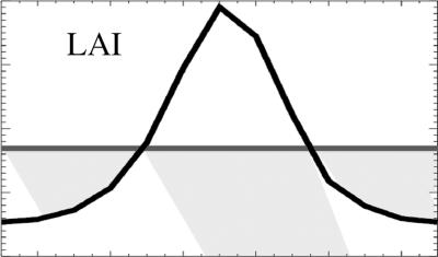
Seasonal cycle of Leaf Area Index (LAI) in central USA prescribed in the HadAM3 model by Lawrence et al. (2003) (black line), and fixed annual mean LAI used in standard version of HadAM3 (grey line).

Figure 9.

Seasonal cycles of (a) 2 m air temperature, (b) latent heat flux and (c) surface albedo in the central USA, with seasonally varying LAI (black line) and fixed LAI (grey line) as shown in figure 8.

Figure 10.

Seasonal cycles of (a) precipitation, (b) evaporation, (c) soil moisture content and (d) runoff in the central USA, with seasonally varying LAI (black line) and fixed LAI (grey line) as shown in figure 8.

Figure 11.

Time-series of European growing season (a) begin date B, (b) end date E and (c) length L. Data from Chmielewski & Rotzer (2001) presented by Lawrence & Slingo (2004).

The effect of vegetation seasonality on climate is important in a climate change context because climate change already appears to be modifying the phenology (timing of key stages of the seasonal cycle) of many species. In temperate regions, there is a general tendency towards earlier bud-burst and leaf-out, and a later leaf fall. Overall, the growing season appears to be lengthening (Chmielewski & Rotzer 2001) (figure 12). Continued climate change may, therefore, lead to further changes in the seasonal cycle of crops, modifying the patterns of change in land surface characteristics and hence providing a feedback on climate change.

Figure 12.

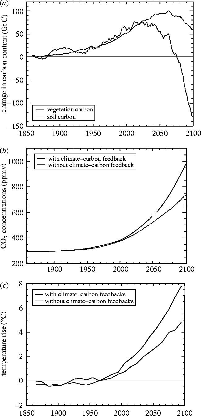
Changes in terrestrial carbon storage simulated over the twenty-first century and the implications for CO₂ rise and climate change, from simulations with the HadCM3LC coupled climate–carbon cycle model driven by the IS92a emissions scenario (Cox et al. 2000). (a) Time-series of changes in global mean vegetation carbon (black) and soil carbon (grey) (Gt C) relative to 1860, in the fully coupled climate–carbon cycle simulation. (b) CO₂ rise (ppmv) simulated as a result of the IS92a emissions scenario, with the effects of climate change on land and ocean carbon fluxes included (black) and excluded (grey). (c) Global land mean temperature rise (°C) relative to 1860, with CO₂ simulated including climate–carbon cycle feedbacks (black) and with CO₂ imposed from projections which exclude climate–carbon cycle feedbacks (grey).

These feedbacks may occur naturally through direct effects of meteorological changes on crops, or via the responses of farmers to observable changes in the growing season. Changes in mean climatic conditions may also exert an influence by altering the viability of particular crops in a given region. For example, a milder UK climate could favour new crops which are not currently widespread, such as grapes or maize. If significant numbers of farmers move towards different crops as a consequence of climate change, this would modify the physical properties of the landscape and act as a further feedback on climate change. As well as modifying properties such as aerodynamic roughness and albedo, changing crop types may also lead to a shift in the proportion of vegetation undergoing C₃ and C₄ photosynthesis. Wheat, for example, undergoes C₃ photosynthesis while maize undergoes C₄ photosynthesis. These photosynthetic pathways lead to different responses of transpiration to changes in CO₂ so may affect the physiological forcing of climate as discussed in §2.

The integration of crop models into GCM land surface schemes would therefore appear to be crucial maintaining consistency between the overlying seasonal climatic conditions and the seasonal state of the cropped landscape (Tsvetsinkaya et al. 2001a,b), both of which may change as a result of climate change.

4. Biogeochemical feedbacks on global climate change from crop-related processes

Enhancement of photosynthesis by increased CO₂ plays an important part in the response of the climate system to anthropogenic carbon emissions (Conroy et al. 1994; Mauney et al. 1994; Kimball et al. 1995; Gitay et al. 2001; Prentice et al. 2001). Along with increased uptake in the oceans, this increased uptake of CO₂ by enhanced photosynthesis provides a partial buffer against the anthropogenic emissions, such that the atmospheric CO₂ concentration, currently, rises at approximately only 50% of the rate of emissions (Prentice 2001). This ‘airborne fraction’ of emissions is a crucial component of projections of future CO₂ rises, and any changes in this fraction could significantly influence the rate of CO₂ rise. A saturation of photosynthesis at high CO₂, as observed in experimental studies, would contribute to an increase in the airborne fraction. Moreover, the return of carbon dioxide to the atmosphere through plant and soil respiration is observed to increase exponentially with temperature (Knorr et al. 2005). These responses have major implications for climate change, as the current 50% airborne fraction may be providing only a temporary buffering of the full effect of anthropogenic CO₂ emissions.

Cox et al. (2000) incorporated models of non-agricultural land and marine ecosystems into a climate model to create a coupled climate model with a fully interactive carbon cycle. Cox et al. (2000) found the saturation of photosynthesis and increase in respiration to significantly increase the rate of CO₂ rise and hence the rate of global warming (figure 12). In a simulation driven by the IPCC IS92a emissions scenario without climate–carbon cycle feedbacks, the atmospheric CO₂ concentration rose from 280 ppmv in 1850 to approximately 750 ppmv by 2100, with a mean warming over land of approximately 5 K. When the feedbacks were included, the same emissions scenario resulted in CO₂ rising to approximately 1000 ppmv by 2100 with global land mean warming being approximately 8 K. Friedlingstein et al. (2001) and Thompson et al. (2004) also found positive feedbacks from the carbon cycle on climate change, but weaker than those found by Cox et al. (2000)

Cox et al. (2000) considered only potential natural vegetation, whereas Friedlingstein et al. (2001) assumed present-day vegetation distributions throughout the simulation. However, in all these studies, the particular responses of croplands were not explicitly considered. The nature of the crops and associated management practices such as irrigation, fertilization and tillage may all affect the local carbon budget and its response to CO₂ rise and climate change. With croplands covering such a significant proportion of the Earth's surface, crop-related processes should be included in coupled climate–carbon cycle models.

Croplands may also play a key role in the response of methane emissions to climate change. In a climate model including wetlands and methane emissions, Gedney et al. (2004) found methane emissions from wetlands to increase as a consequence of climate change, mainly as a result of rising temperatures but partly owing to increases in wetland area (figure 13). The additional emissions and associated radiative forcing were of a similar magnitude to those expected as a direct consequence of human activity in the emissions scenario, suggesting that the standard projections may only account for half of the future methane emissions (Gedney et al. 2004). Rice cultivation may play a significant part in this feedback, with the extent of paddies, the choice of cultivar and other aspects of the management practice all being important. The explicit representation of paddy rice within climate system models may, therefore, be important.

Figure 13.

Feedbacks between climate change and CH₄ emissions from wetlands. (a) CH₄ emissions excluding (solid red line) and including (dashed red line) the effects of climate change on wetland extent and temperature. CO₂ concentrations (blue line) for comparison. (b) Global mean radiative forcing from CH₄ (red lines), CO₂ (blue line) and all species (black line), with effects of climate change on CH₄ emissions excluded (solid lines) and included (dashed lines). (Gedney et al. 2004), British Crown Copyright.

5. Synergistic impacts of climate change and changes in atmospheric composition

Section 2 noted that as well as exerting a radiative forcing on the climate system, increasing concentration of atmospheric CO₂ may also exert a forcing through direct effects on plant physiology. In addition to modifying transpiration, photosynthesis generally increases with CO₂ concentration, a mechanism often termed ‘CO₂ fertilization’.

Cramer et al. (2001) used six Dynamic Global Vegetation Models (DGVMs) to simulate vegetation responses to a scenario of climate change and CO₂ rise over the 21st Century. They found CO₂ fertilization and climate change to interact non-linearly in their influences on natural vegetation. By 2100, climate change alone, generally, led to a negative net atmosphere–land carbon flux or net ecosystem productivity (NEP) which is the difference between the carbon uptake by photosynthesis and the release through plant and soil respiration. However, CO₂ increase alone led to positive NEP. The linear sum of these effects was a general increase in NEP, but in simulations driven by both CO₂ and climate change together, negative NEP was simulated in many parts of the tropics (figure 14). Synergistic effects of climate change and CO₂ rise are already considered in many assessments of future changes in crop production (Matthews et al. 1997; Gitay et al. 2001).

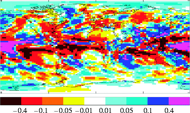
Figure 14.

NEP simulated under changes in CO₂ and climate in various combinations. Column 1: NEP under climate change simulated by the HadCM2 GCM for the IS92a scenarios, with CO₂ fixed at a pre-industrial concentration. Column 2: NEP under CO₂ increasing according to IS92a, under pre-industrial climate. Column 3: NEP under climate change and CO₂ imposed together. Column 4: linear combination of columns 1 and 2. Top row: present-day NEP. Middle row: state simulated for the end of the twenty-first century. Bottom row: state simulated for 100 years after a hypothetical stabilization at 2100. Individual maps are means of the output from six DGVMs. Cramer et al. (2001), copyright Blackwell.

Another atmospheric constituent which directly affects plant productivity is ozone (O₃). Excessive O₃ concentrations near the surface can damage plant cells and therefore reduce productivity, with the risk of decreasing crop yield (McKee & Long 2001; Morgan et al. 2003, 2004) (figure 15). As an illustration of this, Sitch et al. (2005) used an offline vegetation model driven by changes in climate, CO₂ and O₃ consistent with the IS92a emissions scenario, and compared the terrestrial carbon storage in simulations with and without O₃ physiological effects. Ozone concentrations were projected to increase by 10–20% over the most populated parts of the temperate and tropical regions, and this was simulated to reduce terrestrial carbon storage by up to 4 kg C m⁻² in the eastern USA, Europe, north and southeast Asia and the tropics, a reduction of approximately 25% (figure 16). When O₃ effects were investigated with and without CO₂ effects, it was found that O₃ damage was reduced under higher CO₂ concentrations as a result of CO₂-induced stomatal closure reducing the flux of O₃ into stomatal cavities. However, in the one case where this synergism was investigated with a field experiment, this amelioration of O₃ effects by CO₂ was not observed (S. Long, personal communication).

Figure 15.

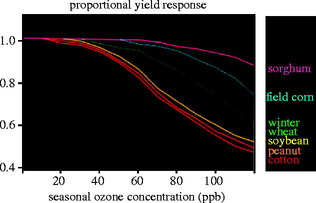
Yield response of selected crops to ozone.

Figure 16.

Simulated gross primary productivity at 2100 under climate change and CO₂ rise, with (a) ozone fixed at present-day concentrations and (b) varying according to the emissions scenario. Sitch et al. (2005), British Crown Copyright.

The various human perturbations to the climate system therefore have the potential to produce major impacts either individually or in combination. The combined effect of these perturbations acting together may be very different to the linear sum of the individual perturbations acting in isolation. Crop models used for climate change impacts assessments should therefore consider the other effects of changes in atmospheric composition which act directly on crop physiology.

6. Interactions between land use change, crop responses and other impacts sectors.

Sections 2 and 3 discussed how crop changes can modify the surface water budget. As well as affecting climate, surface water budget changes will also affect hydrology, so changes in crop characteristics may modify the hydrological impacts of climate change such as the risks of drought and flooding. Changes between forest and cropland, changes in the seasonal cycle of crop leaf area, and changes in stomatal conductance may all influence the hydrological responses to climate change in addition to the better known effects of changes in precipitation and evaporation arising from radiative forcing.

Major changes in land cover such as conversion of forest to croplands or pasture have been shown to potentially impact evaporation and precipitation, so it follows that such activities would also impact runoff. Lean & Rowntree (1993) found an 8% reduction in simulated runoff from Amazonia following complete deforestation, as a result of decreased precipitation outweighing the decrease in evaporation. However, surface runoff was simulated to increase by 27% at the expense of sub-surface runoff, because infiltration rates were assumed to decrease after deforestation. Infiltration rates in forest soils were assumed to be high due to the presence of litter and tree root systems, while infiltration in land deforested for pasture was assumed to be low due to soil compaction during the deforestation process and by the presence of livestock. Similarly, Twine et al. (2004) found conversion from forest to cropland in the southern USA to increase runoff by up to 45% in winter, while conversion from natural grassland to cropland was found to decrease summer runoff by 25% in the northern USA. Since land cover changes such as deforestation for cultivation or pasture are included in the generation of climate change scenarios through their contribution to emissions and uptake of CO₂, a consistent approach to hydrological impacts studies in agricultural areas will require consideration of the effects of converting between forest and croplands on runoff.

A further mechanism through which croplands may modify hydrological impacts is via the response of the crop transpiration to elevated CO₂ concentrations. Reduced transpiration implies an increase in the proportion of water remaining at the land surface, and this implies an increase in runoff as a consequence of the physiological impact of rising CO₂ on vegetation (Wigley & Jones 1985).

In simulations with DGVMs including hydrology under the IS92a scenario of CO₂ increase, ignoring any associated radiatively forced climate change, Cramer et al. (2001) found all but one of their models to simulate an increase in global runoff due to the physiological effects of CO₂ rise alone. The simulated changes in runoff ranged from −3 to +47% (figure 17). It should be noted that the simulations included dynamic vegetation, so the physiological forcing could also exert an impact through changes in leaf area and vegetation distribution. This is important, because such changes in vegetation structure may affect climate through changes in land surface properties as well as through stomatal closure (Betts et al. 1997). The changes in runoff, therefore, arose from physiological impacts on plant stomata, leaf area and vegetation distribution.

Figure 17.

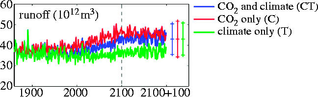
Time-series of global mean runoff simulated with six DGVMs, with climate change alone (green line), CO₂ physiological forcing alone (red line) and both CO₂ and climate change (blue line). Cramer et al. (2001), copyright Blackwell.

With the DGVMs driven by climate change alone without CO₂ physiological forcing, Cramer et al. (2001) simulated a change in runoff of −1 to +9%. When both climate change and physiological forcing were included, the changes in runoff were +1 to +45% (figure 17). This suggests that rising CO₂ could increase global mean runoff more through physiological forcing of transpiration than radiatively forced climate change. In regions where radiatively forced climate change does not significantly increase local precipitation, increased runoff may still occur as a result of physiological forcing.

Cramer et al. (2001) only considered the effects of natural vegetation responses on hydrology, using models which simulated potential vegetation which is often forest in regions which are currently under agriculture. The importance of stomatal resistance in determining the overall flux of moisture between the land and the atmosphere in a given location may vary according to the character of the land cover, particularly its aerodynamic roughness length. A forested landscape with a high roughness length may induce a high degree of turbulence and hence contribute a small aerodynamic resistance to the turbulent transfer of moisture, and hence changes in stomatal resistance due to CO₂ changes may be more significant for a forest than for croplands which generally have a relatively small aerodynamic roughness length. The processes investigated by Cramer et al. (2001) should therefore be further studied with models of the interactions between climate, land cover and surface hydrology. Moreover, the stomatal response to CO₂ may itself vary according to the particular crop type present. Therefore, assessments of the hydrological impacts of CO₂-induced climate change, such as changes in drought and flood risk, should consider the physiological responses of vegetation including crops.

7. Difficulties with applying climate model output to offline impacts studies

As well as omitting a number of key processes as described in §§2–6, the current practice of applying GCM or RCM output to separate (‘offline’) crop models presents a number of practical difficulties. In particular, the quantity of output data is vast. A typical GCM will output approximately 200 variables on more than 15 000 grid points with 20–60 atmospheric layers at each point. The models typically use a 30 min timestep and perform simulations of up to 250 years in length, with large numbers of simulations being employed to examine multiple forcing scenarios and investigate model uncertainties with multi-member ensembles of 16–128 simulations per scenario. Contemporary modelling studies produce several tens of terabytes of output, and with current technology this quantity of data is not easy or cheap to store, transmit and process in its entirety.

This difficulty can be partly addressed through the use of spatial and temporal averages and statistics on the extreme values. However, crop models often require input data at a high spatial and temporal resolution. For example, short periods of heat stress can be critical (Matsui & Horie 1992; Ferris et al. 1998; Vara Prasad et al. 2000), but may not be adequately represented in averaged data. Short-time-scale detail is often regenerated from the average GCM and RCM output with ‘weather generator’ software which uses information on the statistics of weather variability (Soltani et al. 2000). The high temporal resolution data produced by the climate models is, therefore, often effectively discarded and then regenerated using statistical techniques. However, this technique relies on the assumption of stationarity in the climate system which may not always be valid (Challinor et al. 2005) so the resulting crop simulation may not be the same as that which would be obtained by driving the crop model with the original high-resolution climate data. This would be avoided if the crop processes were simulated within the climate model itself.

A further issue is that output variables produced by climate models do not always include the input variables required by crop models, meaning that further processing of data is required in order to translate climate model output into crop model input. This may present problems when the processes are non-linear, such as potential evapotranspiration (Plentinger & Penning de Vries 1996) or thermal time (Challinor et al. 2004), as the use of mean data may not adequately represent the true implications of the original high temporal resolution climate model data (Loomis & Connor 1992; Osborne 2004). In many cases, such processes could be simulated by the climate model itself, but often are not because they do not directly affect the climate. Again, this problem would be avoided if the climate models were used to generate output variables of direct relevance to impacts studies.

Another problem with using crop models driven by climate model output is that the crop models often represent some of the same processes as the climate models, but with different methods. For example, atmospheric models simulate surface moisture fluxes in order to maintain a conservative water cycle (e.g. Cox et al. 1999). Many crop models also simulate surface moisture fluxes, but often at a higher spatial resolution and/or with different treatments of the details of processes such as transpiration (e.g. Trevasso & Delécolle 1995). If the moisture fluxes simulated by a crop model are different to those simulated by the atmospheric model from which its input data is derived, the meteorology may be inconsistent with the crop simulation. These inconsistencies can be reduced if the crop and climate simulations are at the same resolution (Hansen & Jones 2000; Challinor et al. 2003; Donner & Kucharik 2003; Donner et al. 2004) or avoided altogether if the crop model forms an integral part of the climate model land surface scheme (Osborne 2004).

The use of separate climate models and impacts models, with large quantities of data being transferred in between, can lead to a long delay between producing climate model output and obtaining impacts results. Since both fields are evolving rapidly in parallel, this creates difficulties in producing an internally consistent assessment of the state-of-the-art projections of climate change and its impacts. For example, the IPCC assessment reports for the physical science and impacts aspects of climate change are written concurrently, which means that the impacts projections being assessed may not have been produced with the climate models being assessed at the same time. Although this is a recognized problem and steps are taken to ensure maximum consistency under the current constraints, this problem would be easier to address if there were a shorter delay between the production of climate model output and impacts results. The use of a crop model implemented within a climate model would eliminate this delay.

8. Challenges for a coupled climate–crop model

Sections 3–7 have demonstrated the need for a more integrated approach to the modelling of climate change and its impacts on crop production. The most complete integration would be achieved by full coupling of a crop model to a climate model with sufficient resolution and complexity to adequately represent climatic processes such as precipitation which are critical to crop production, therefore, allowing for the full range of interactions described above. However, this is not trivial as there are a number of potential difficulties associated with such integration.

One difficulty is that complex climate models such as GCMs and RCMs require significant computing resources to perform even one simulation, with century-scale simulations requiring between 1 and 6 months of real time depending on the computing platform. This may, therefore, impose a practical constraint on the number of simulations which can be performed, limiting the ability to explore the implications of uncertainties in the driving scenarios or model formulation. It will often be necessary to explore uncertainties associated more directly with the crops than with the atmosphere, such as uncertainties in future management practice, crop modelling methodology or crop model parameter values. In a fully coupled climate–crop model, exploration of such uncertainties would require multiple simulations of the entire climate modelling system, and implementation of different crop models or model versions within the climate model. This would require significant investment of resources for programming and significant periods of time between implementation and final results. In many cases, it may be judged more efficient to seek initial guidance on the importance of the uncertainties through the use of a crop model separate from the GCM and driven by GCM output data.

Another difficulty is that climate models often feature significant biases in their simulations of present-day climate in comparison with observations, particularly at the regional scale (Slingo et al. 2003). In offline impacts modelling studies, this is typically addressed by taking the simulated climate change anomalies from the climate model and adding these to observed climatology, to generate bias-corrected data which is then provided to the impacts model. The biases are usually identified in climate model output data averaged over periods of days or months, rather than in the timestep data, since observational data are more, generally, available and easier to process at daily and monthly time-scales. Although, this approach relies on the assumption that the bias in the present-day simulation represents a systematic bias which continues into the future simulation, which may not actually be the case, it does provide one means to avoid the generation of unrealistic impacts simulations at the present-day. Such a correction technique may be difficult to apply to a fully coupled climate–crop model because it would involve the identification of biases in the timestep data which would require large quantities of observational data at the time-scale of minutes to one hour.

A further issue is the disparity in temporal and spatial scales between typical examples of climate and crop models (Osborne 2004). As noted above, climate models typically operate on timesteps of minutes (5–30 min in current examples) whereas crop models often require daily or monthly data. Conversely, the spatial resolution of climate models is, generally, much coarser than that of crop models, with current climate models operating at resolutions of 50 km to 2° while crop models are often designed to operate at scales of metres or a few kilometres. Tsvetsinkya et al. (2003) and Carborne et al. (2003) found that crop models can produce significantly different results at different spatial scales. Offline impacts studies usually down-scale the climate data to a spatial scale appropriate to the crop model, generally, assuming uniform relationships between large-scale and small-scale features of climate and weather. Full coupling of climate and crop models must either find some way of calibrating these scale relationship at the level of the climate model timestep, or use models which are specifically designed to operate at common scales (Hansen & Jones 2000; Donner & Kucharik 2003; Donner et al. 2004; Challinor et al. 2004).

9. Options for a more integrated approach

Given the potential difficulties with coupling crop models to climate models, the challenge is to find the most appropriate method or combination of methods for modelling the impacts of climate change on crop production which are both realistic and practical. The methods need to capture the interactions between the physical and chemical states of the atmosphere, land surface properties, crop physiological processes, soil processes and hydrology at the appropriate spatial and temporal scales, and also represent direct human interventions such as land cover conversion and crop management.

One option, the online impacts approach, is to implement a crop model as an integral component of a climate model (Osborne 2004). This is probably the only way to account for feedbacks from crop changes to climate, and is also an effective means of overcoming the difficulty in transferring large quantities of timestep data between models. If other impacts models, such as hydrological models, are also implemented in the climate model, this also facilitates an integrated treatment of climate change impacts on crops and other sectors. Furthermore, the online approach would allow impacts results to be obtained at the same time as the climate change results, rather than some time later. However, some method is required for dealing with the disparity of scales, such as designing a crop model to operate at climate model scales (Challinor et al. 2003). Furthermore, the biases in the climate simulation either need to be corrected while the simulation is in progress, or their presence simply accepted. In the latter case, the trade-off between these biases and the biases arising from neglecting feedbacks needs to be judged (Osborne 2004).

Another option is to continue with the offline impacts approach, but with greater focus on the end product. This involves ensuring that the climate model outputs meet the input needs of the crop models, and also that the experimental design is appropriate to the question being addressed. The output data needs can be addressed as part of the development of the climate model by considering the crop models to which the output will be applied and implementing code to diagnose the appropriate quantities in the climate model while the simulation is in progress. For example, potential evapotranspiration and thermal time can easily be simulated/calculated within the climate model land surface scheme. The experimental design should be drawn-up with full consideration of the reason for performing the impacts study; if the purpose is to assess the impacts of radiatively forced climate change alone, then the climate models can be driven by scenarios of greenhouse gas and aerosols concentrations. If, however, the purpose is to assess climate change impacts in the context of other aspects of global change, these other aspects must be taken into account in the experimental design. Section 2 discussed the need to consider land cover change as a driver of climate change, especially at the global scale. This can be accounted for in GCMs and RCMs by modifying the vegetation distribution and properties within the land surface scheme, according to scenarios of future land use change which are often implied by the emissions scenarios (Feddema et al. in press; Johns et al. 2005). The regional climates provided to offline crop models would therefore be consistent with any changes in croplands and other land cover implied by the global change scenarios used to provide emissions.

While the offline approach neglects any feedbacks from crops to climate, and may still present difficulties in transferring large quantities of data, it is more flexible than the online approach in allowing more crop model simulations to be driven with one climate model simulation. This is valuable for investigating the robustness of simulated crop responses efficiently, assuming that crop–climate feedbacks are of secondary importance for this robustness. The offline approach also allows biases in the climate simulation to be accounted for more easily.

Current offline impacts studies typically neglect the interactions between different impacts sectors because separate models (usually developed by different research groups) are used to study each sector. However, this need not necessarily be the case, as a number of impacts models could be implemented in a land surface model outside of a GCM. If such a model were driven offline by climate model output, this would offer the advantages of the offline approach whilst also allowing an integrated treatment of a number of impacts sectors such as crops, hydrology and natural ecosystems as discussed in §6. This would allow for the models of the different sectors to consider the constraints imposed by the other sectors; for example, the available water may need to be shared amongst the crop, water resources and natural ecosystem models with the demands of each affecting the supply to the others.

The use of a land surface model as a framework for impacts modelling would potentially allow greater consistency between the treatments of processes in the impacts and climate models. If the underlying land surface model were the same as that used in the climate, albeit with some additional processes included, the simulation of the key surface processes is likely to be similar in the offline model and climate model. This would help to reduce the problem of inconsistencies discussed in §7. With careful experimental design of both the climate modelling and offline land surface modelling aspects, the use of a crop model within an integrated offline land surface model could also address the issue of land cover change forcing discussed in §2 and the synergistic drivers of impacts discussed in §5.

Nevertheless, the integrated offline model would still neglect feedbacks between crops and climate, so the climate and crop simulations may not be truly consistent with each other. The issues discussed in §§2 and 4 would, therefore, remain. Ultimately, a fully coupled climate–crop model with minimal biases would be expected to provide the most comprehensive and internally consistent simulation of global change impacts on crops. The availability of computing resources would provide the main limitation on a full exploration of uncertainties in predictions with such a model.

10. Conclusions and recommendations

A more integrated approach to climate–crop modelling would increase the robustness of projections of the impacts of climate change on crop production and also the projections of climate change itself. There are, currently, a number of challenges in coupling crop models to climate models, but such a coupling is the only way to achieve a fully consistent view of the effects of global change on crop production. We, therefore, require a strategy for progress towards a fully integrated climate–crop modelling system in parallel with the production of new insights using more practical and immediately accessible tools.

On the basis of the arguments presented here, I recommend a strategy consisting of three parallel streams of model development and application.

1. The first stream consists of the further development of global and RCMs for use with offline crop models, taking full account of the end use when developing the outputs of the model and experimental design of the simulations. This could allow for other climate forcings such as land cover change and provide specific outputs for driving crop models.

2. The second stream involves the implementation of crop models into offline land surface models, to allow interaction with models of other impacts. Careful use in conjunction with the climate models of stream 1 could allow for multiple stresses on crops and consistency between cropland changes and climate.

3. The third stream involves the implementation of crop models within climate models to allow a fully interactive representation of global change impacts on crops (e.g. Osborne 2004). This is more complete than the models developed in streams 1 and 2, but present its own drawbacks.

In practice, progress is likely to be best maintained by pursuing all three streams in parallel.

References

- Alcamo J, Kreileman G.J.J, Bollen J.C, van den Born G.J, Gerlagh R, Krol M.S, Toet A.M.C, De Vries H.J.M. Baseline scenarios of global environmental change. In: Alcamo J, Leemans R, Kreileman E, editors. Results from the IMAGE2.1 model. Elsevier Science; Amsterdam: 1998. pp. 97–139. [Google Scholar]
- Betts R.A. Self-beneficial effects of vegetation on climate in a General Circulation Model. Geophys. Res. Lett. 1999;26:1457–1460. doi:10.1029/1999GL900283 [Google Scholar]
- Betts R.A. Offset of the potential carbon sink from boreal forestation by decreases in surface albedo. Nature. 2000;408:187–190. doi: 10.1038/35041545. doi:10.1038/35041545 [DOI] [PubMed] [Google Scholar]
- Betts R.A. Biogeophysical impacts of land use on present-day climate: near-surface temperature change and radiative forcing. Atmos. Sci. Lett. 2001;2:39–51. doi:1006/asle20010023 [Google Scholar]
- Betts R.A, Cox P.M, Lee S.E, Woodward F.I. Contrasting physiological and structural vegetation feedbacks in climate change simulations. Nature. 1997;387:796–799. doi:10.1038/42924 [Google Scholar]
- Betts R.A, Cox M, Woodward F.I. Simulated responses of potential vegetation to doubled-CO2 climate change and feedbacks on near-surface temperature. Global Ecol. Biogeogr. 2000;9:171–180. doi:10.1046/j.1365-2699.2000.00160.x [Google Scholar]
- Betts R.A, Cox P.M, Collins M, Harris P.P, Huntingford C, Jones C.D. The role of ecosystem–atmosphere interactions in simulated Amazonian precipitation decrease and forest dieback under global climate warming. Theor. App. Climatol. 2004;78:157–175. [Google Scholar]
- Bonan G.B, Pollard D, Thompson S.L. Effects of boreal forest vegetation on global climate. Nature. 1992;359:716–718. doi:10.1038/359716a0 [Google Scholar]
- Boucher O, Myhre G, Myhre A. Direct influence of irrigation on atmospheric water vapour and climate. Climate Dyn. 2004;22:597–603. doi:10.1007/s00382-004-0402-4 [Google Scholar]
- Bounoua L, DeFries R, Collatz G.J, Sellers P, Khan H. Effects of land cover conversion on surface climate. Climatic Change. 2002;52:29–64. doi:10.1023/A:1013051420309 [Google Scholar]
- Brovkin V, Ganapolski A, Claussen M, Kubatzki C, Petoukhov V. Modelling climate response to historical land cover change. Global Ecol. Biogeogr. 1999;8:509–517. doi:10.1046/j.1365-2699.1999.00169.x [Google Scholar]
- Carborne G.C, Kiechle W, Locke C, Mearns L.O, McDaniel L, Downton M.W. Response of soybean and sorghum to varying spatial scales of climate change scenarios in the Southeastern United States. Climatic Change. 2003;60:73–98. doi:10.1023/A:1026041330889 [Google Scholar]
- Challinor A.J, Slingo J.M, Wheeler T.R, Craufurd P.Q, Grimes D.I.F. Toward a combined seasonal weather and crop productivity forecasting system: determination of the working spatial scale. J. Appl. Meteorol. 2003;42:175–192. doi:10.1175/1520-0450(2003)042<0175:TACSWA>2.0.CO;2 [Google Scholar]
- Challinor A.J, Wheeler T.R, Slingo J.M, Craufurd P.Q, Grimes D.I.F. Design and optimisation of a large-area process-based model for annual crops. Agric. Forest Meteorol. 2004;124:99–120. doi:10.1016/j.agrformet.2004.01.002 [Google Scholar]
- Challinor A.J, Wheeler T.R, Slingo J.M, Craufurd P.Q, Grimes D.I.F. Simulation of crop yields using the ERA40 re-analysis: limits to skill and non-stationarity in weather-yield relationships. J. Appl. Meteorol. 2005;44:516–531. doi:10.1175/JAM2212.1 [Google Scholar]
- Charney J.G. Dynamics of deserts and droughts in the sahel. Q. J. R. Meteorol. Soc. 1975;101:193–202. doi:10.1256/smsqj.42801 [Google Scholar]
- Chmielewski F.M, Rotzer T. Response of tree phenology to climate change across Europe. Agric. Forest Meteorol. 2001;108:101–112. doi:10.1016/S0168-1923(01)00233-7 [Google Scholar]
- Conroy J.P, Seneweera S, Basra A.S, Rogers G, Nissenwooller B. Influence of rising atmospheric CO2 concentrations and temperature on growth, yield and grain quality of cereal crops. Aust. J. Plant Physiol. 1994;21:741–758. [Google Scholar]
- Cox P.M, Betts R.A, Bunton C.B, Essery R.L.H, Rowntree P.R, Smith J. The impact of new land surface physics on the GCM simulation of climate and climate sensitivity. Climate Dyn. 1999;15:183–203. doi:10.1007/s003820050276 [Google Scholar]
- Cox P.M, Betts R.A, Jones C.D, Spall S.A, Totterdell I.J. Acceleration of global warming due to carbon-cycle feedbacks in a coupled climate model. Nature. 2000;408:184–187. doi: 10.1038/35041539. doi:10.1038/35041539 [DOI] [PubMed] [Google Scholar]
- Cramer W, et al. Global response of terrestrial ecosystem structure and function to CO2 and climate change: results from six dynamic global vegetation models. Global Change Biol. 2001;7:357–374. doi:10.1046/j.1365-2486.2001.00383.x [Google Scholar]
- Döll P, Siebert S. A digital global map of irrigated areas. ICID J. 2000;49:55–66. [Google Scholar]
- Döll P, Siebert S. Global modeling of irrigation water requirements. Water Resour. Res. 2002;38:1037. [Google Scholar]
- Donner S.D, Kucharik C.J. Evaluating the impacts of land management and climate variability on crop production and nitrate export across the Upper Mississippi Basin. Global Biogeochem. Cycles. 2003;17:1085. doi:10.1029/2001GB001808 [Google Scholar]
- Donner S.D, Kucharik C.J, Foley J.A. The impact of changing land use practices on nitrate export by the Mississippi River. Global Biogeochem. Cycles. 2004;18:GB1028. doi:10.1029/2003GB002093 [Google Scholar]
- Douville H, Royer F.J. Influence of the temperate and boreal forests on the Northern Hemisphere climate in the Météo-France climate model. Climate Dyn. 1997;13:57–74. [Google Scholar]
- Feddema, J., Oleson, K., Bonan, G., Mearns L., Washington W., Meehl, G., Nychka, D. In press. A comparison of a GCM response to historical anthropogenic land cover change and model sensitivity to uncertainty in present-day land cover representations. Climate Dyn (doi:10.1007/s00382-005-0038-z)
- Ferris R, Ellis R.H, Wheeler T.R, Hadley P. Effect of high temperature stress at anthesis on grain yield and biomass of field-grown crops of wheat. Ann. Bot. 1998;82:631–639. doi:10.1006/anbo.1998.0740 [Google Scholar]
- Field C, Jackson R, Mooney H. Stomatal responses to increased CO2: implications from the plant to the global scale. Plant, Cell Environ. 1995;18:1214–1255. [Google Scholar]
- Friedlingstein P, Bopp L, Ciais P, Dufresne J.-L, Fairhead L, LeTreut H, Monfray P, Orr J.C. Positive feedback between future climate change and the carbon cycle. Geophys. Res. Lett. 2001;28:1543–1546. doi:10.1029/2000GL012015 [Google Scholar]
- Gedney N, Cox P.M, Huntingford C. Climate feedback from wetland methane emissions. Geophys. Res. Lett. 2004;31:L20503. doi:10.101029/2004GL020919 [Google Scholar]
- Gitay H, et al. Climate Change 2001: impacts, adaptation and vulnerability, pp. 235–342. Contribution of Working Group II to the Third Assessment of the Intergovernmental Panel on Climate Change. Cambridge University Press; Cambridge, UK: 2001. Ecosystem and their goods and services. [Google Scholar]
- Govindasamy B, Duffy P.B, Caldeira K. Land use changes and Northern Hemisphere cooling. Geophys. Res. Lett. 2001;28:291–294. doi:10.1029/2000GL006121 [Google Scholar]
- Hansen J.W, Jones J.W. Scaling-up crop models for climate variability applications. Agric. Syst. 2000;65:43–72. doi:10.1016/S0308-521X(00)00025-1 [Google Scholar]
- Harding R.J, Pomeroy J.W. The energy balance of the winter boreal landscape. J. Climate. 1996;9:2778–2787. doi:10.1175/1520-0442(1996)009<2778:TEBOTW>2.0.CO;2 [Google Scholar]
- Johns, T. C. et al Submitted. The new Hadley Centre climate model HadGEM1 (2005) Evaluation of coupled simulations in comparison to previous models. J. Climate
- Kimball B.A, Pinter P.J, Jr, Garcia R.L, LaMorte R.L, Wall G.W, Hunsaker D.J, Wechsung G, Wechsung F, Karschall T. Productivity and water use of wheat undser free-air CO2 enrichment. Global Change Biol. 1995;1:429–442. [Google Scholar]
- Kleidon A, Heimann M. Assessing the role of deep rooted vegetation in the climate system with model simulations: mechanism, comparison to observations and implications for Amazonian deforestation. Climate Dyn. 2000;16:183–199. doi:10.1007/s003820050012 [Google Scholar]
- Knorr W, Prentice I.C, House J.I, Holland E.A. Long-term sensitivity of soil carbon turnover to warming. Nature. 2005;433:298–301. doi: 10.1038/nature03226. doi:10.1038/nature03226 [DOI] [PubMed] [Google Scholar]
- Lawrence D.M, Slingo J.M. An annual cycle of vegetation in a GCM. Part II: global impacts on climate and hydrology. Climate Dyn. 2004;22:107–122. doi:10.1007/s00382-003-0367-8 [Google Scholar]
- Lean J, Rowntree P.R. A GCM simulation of the impact of Amazonian deforestation on climate using an improved canopy representation. Q. J. R. Meteorol. Soc. 1993;119:509–530. doi:10.1256/smsqj.51108 [Google Scholar]
- Lean J, Rowntree P.R. Understanding the sensitivity of a GCM simulation of Amazonian deforestation to the specification of vegetation and soil characteristics. J. Climate. 1997;10:1216–1235. doi:10.1175/1520-0442(1997)010<1216:UTSOAG>2.0.CO;2 [Google Scholar]
- Lean J, Warrilow A. Simulation of the regional climatic impact of Amazon deforestation. Nature. 1989;342:411–413. doi:10.1038/342411a0 [Google Scholar]
- Loomis R.S, Connor D.J. Cambridge University Press; Cambridge, UK: 1992. Crop ecology. [Google Scholar]
- Matsui T, Horie T. Effect of elevated CO2 and high temperature on growth and yield of rice. II. Sensitive period and pollen germination rate in high temperature on growth sterility of rice spikelets at flowering. Jpn J. Crop Sci. 1992;61:148–149. [Google Scholar]
- Matthews R.B, Kropff M.J, Horie T, Bachelet D. Simulating the impact of climate change on rice production in Asia and evaluating options for adaptation. Agric. Syst. 1997;54:399–425. doi:10.1016/S0308-521X(95)00060-I [Google Scholar]
- Mauney J.R, Kimball B.A, Pinter P.J, LaMorte R.L, Lewin K.F, Nagy J, Hendrey G.R. Growth and yield of cotton in response to a free-air carbon dioxide enrichment (FACE) environment. Agric. Forest Meteorol. 1994;70:49–67. doi:10.1016/0168-1923(94)90047-7 [Google Scholar]
- McKee I.F, Long S.P. Plant growth regulators control ozone damage to wheat yield. New Phytologist. 2001;152:41–51. doi: 10.1046/j.0028-646x.2001.00207.x. doi:10.1046/j.0028-646x.2001.00207.x [DOI] [PubMed] [Google Scholar]
- Morgan P.B, Ainsworth E.A, Long S.P. How does elevated ozone impact soybean? A meta-analysis of photosynthesis, growth and yield. Plant, Cell Environ. 2003;26:1317–1328. doi:10.1046/j.0016-8025.2003.01056.x [Google Scholar]
- Morgan P.B, Bernacchi C.J, Ort D.R, Long S.P. An in vivo analysis of the effect of season-long open-air elevation of ozone to anticipated 2050 levels on photosynthesis in soybean. Plant Physiologist. 2004;135:2348–2357. doi: 10.1104/pp.104.043968. doi:10.1104/pp.104.043968 [DOI] [PMC free article] [PubMed] [Google Scholar]
- Nakićenović N.J, et al. A special report of Working Group III of the IPCC. Cambridge University Press; Cambridge, UK: 2000. Special report on emissions scenarios; p. 599. [Google Scholar]
- Osborne, T. M. 2004 Towards an integrated approach to simulating crop–climate interactions Ph.D. Thesis, University of Reading.
- Pielke R.A. Overlooked issues in the US National climate and IPCC assessments. Climatic Change. 2002;52 [Google Scholar]
- Pielke R.A, Marland G, Betts R.A, Chase T.N, Eastman J.L, Niles J.O, Niyogi D.S, Running S.W. The influence of land-use change and landscape dynamics on the climate system—relevance to climate change policy beyond the radioactive effect of greenhouse gases. Phil. Trans. R. Soc. A. 2002;360:1705–1719. doi: 10.1098/rsta.2002.1027. doi:10.1098/rsta.2002.1027 [DOI] [PubMed] [Google Scholar]
- Plentinger M.C, Penning de Vries F.W.T, editors. CAMASE, Register of Agro-ecosystems Models. DLO-Research Institute for Agrobiology and Soil Fertility (AB-DLO); 1996. [Google Scholar]
- Prentice I.C. The carbon cycle and atmospheric carbon dioxide. In: Houghton J.T, Ding Y, Griggs D.J, Noguer M, van der Linden P, Dai X, Maskell K, Johnson C.I, editors. Climate Change 2001: the scientific basis. Contribution of Working Group I to the Third Assessment Report of the Intergovernmental Panel on Climate Change. Cambridge University Press; Cambridge, UK: 2001. pp. 183–237. [Google Scholar]
- Prentice I.C, Farquhar G.D, Fasham M.J.R, Goulden M.L, Heimann M, Jaramillo V.J, Kheshgi H.S, Le Quere C, Scholes R.J, Wallace D.W.R. The carbon cycle and atmospheric carbon dioxide. In: Houghton J.T, Ding Y, Griggs D.J, Noguer M, van der Linden P, Dai X, Maskell K, Johnson C.I, editors. Climate Change 2001: The scientific basis. Contribution of Working Group I to the Third Assessment Report of the Intergovernmental Panel on Climate Change. ch. 3. Cambridge University Press; Cambridge, UK: 2001. pp. 183–237. [Google Scholar]
- Ramankutty N, Foley J.A. Estimating historical changes in global land cover: croplands from 1700 to 1992. Global Biogeochem. Cycles. 1999;13:997–1027. doi:10.1029/1999GB900046 [Google Scholar]
- Salati E, Vose P.B. Amazon Basin: a system in equilibrium. Nature. 1984;225:129–138. doi: 10.1126/science.225.4658.129. [DOI] [PubMed] [Google Scholar]
- Sellers P.J, et al. Comparison of radiative and physiological effects of doubled atmospheric CO2 on climate. Science. 1996;271:1402–1406. [Google Scholar]
- Sitch S, Cox P, Huntingford C, Collins W, Hemming D, Gedney N. Contract deliverable 08.04.04, DEFRA Climate Prediction Programme. 2005. Report on possible impacts of tropospheric ozone changes on land carbon uptake. [Google Scholar]
- Slingo J.M, et al. Research at GCM on identifying and understanding model systematic errors. Technical Report, NCAS Centre for Global Atmospheric Modelling. 2003. How good is the Hadley Centre climate model? [Google Scholar]
- Soltani A, Latifi N, Nasiri M. Evaluation of WGEN for generating long term weather data for crop simulations. Agric. Forest Meteorol. 2000;102:1–12. doi:10.1016/S0168-1923(00)00100-3 [Google Scholar]
- Thomas G, Rowntree P.R. The boreal forests and climate. Q. J. R. Meteorol. Soc. 1992;118:469–497. doi:10.1256/smsqj.50504 [Google Scholar]
- Thompson S.L, Govindasamy B, Mirin A, Caldeira K, Delire C, Milovich J, Wickett M, Erickson D. Quantifying the effects of CO2-fertilized vegetation on future climate. Geophys. Res. Lett. 2004;31:33. [Google Scholar]
- Trevasso M.I, Delécolle R. Adaptation of the CERES-wheat model for large area yield estimation in Argentina. Eur. J. Agronomy. 1995;4:347–353. [Google Scholar]
- Tsvetsinkya E.A, Mearns L.O, Mavromatis T, Gao W, McDaniel L, Downton M.W. The effect of spatial scale of climatic change scenarios on simulated maize, winter wheat and rice production in the Southeastern United States. Climatic Change. 2003;60:37–71. doi:10.1023/A:1026056215847 [Google Scholar]
- Tsvetsinskaya E.A, Mearns L.O, Easterling W.E. Investigating the effect of seasonal plant growth and development in three-dimensional atmospheric simulations. Part I: Simulation of surface fluxes over the growing season. J. Climate. 2001a;14:692–709. doi:10.1175/1520-0442(2001)014<0692:ITEOSP>2.0.CO;2 [Google Scholar]
- Tsvetsinskaya E.A, Mearns L.O, Easterling W.E. Investigating the effect of seasonal plant growth and development in three-dimensional atmospheric simulations. Part II: Atmospheric response to crop growth and development. J. Climate. 2001b;14:711–729. doi:10.1175/1520-0442(2001)014<0711:ITEOSP>2.0.CO;2 [Google Scholar]
- Twine T.E, Kucharik C.J, Foley J.A. Effects of land cover change on the energy and water balance of the Mississippi River basin. J. Hydrometeorol. 2004;5:640–655. doi:10.1175/1525-7541(2004)005<0640:EOLCCO>2.0.CO;2 [Google Scholar]
- Vara Prasad P.V, Craufurd P.Q, Summerfield R.J, Wheeler T.R. Effects of short episodes of heat stress on flower production and fruit-set of groundnut (arachis hypogea L.) J. Exp. Botany. 2000;51:777–784. doi: 10.1093/jexbot/51.345.777. doi:10.1093/jexbot/51.345.777 [DOI] [PubMed] [Google Scholar]
- Watson R.T, Noble I.R, Bolin B, Ravindranath N.H, Verardo D.J, Dokken D.J, editors. Land use, land-use change and forestry. A Special Report of the IPCC. Cambridge University Press; Cambridge, UK: 2000. p. 337. [Google Scholar]
- Wigley T.M.L, Jones P.D. Influences of precipitation changes and direct CO2 effects on streamflow. Nature. 1985;314:149–152. doi:10.1038/314149a0 [Google Scholar]