Aspects of climate change prediction relevant to crop productivity

Abstract

Projected changes in surface climate are reviewed at a range of temporal scales, with an emphasis on tropical northern Africa—a region considered to be particularly vulnerable to climate change. Noting the key aspects of ‘weather’ affecting crop yield, we then consider relevant and projected change using output from a range of state of the art global climate models (GCMs), and for different future emission scenarios. The outputs from the models reveal significant inter-model variation in the change expected by the end of the twenty-first century for even the lowest IPCC emission scenario. We provide a set of recommendations on future model diagnostics, configurations and ease of use to close further the gap between GCMs and smaller-scale crop models. This has the potential to empower countries to make their own assessments of vulnerability to climate change induced periods of food scarcity.

1. Introduction and overview

(a) Issues of large-scale climate change

The Earth achieves thermal equilibrium by balancing the net incoming solar radiation received from the Sun, with the infra-red radiation emitted back to space (see Houghton 2002). This infra-red radiation is primarily blackbody radiation emitted by the Earth's surface and by clouds, but some infrared radiation is intercepted by the so-called atmospheric ‘greenhouse gases’ and absorbed at particular frequencies determined by their molecular structure. Only some of this absorbed energy is re-emitted by the greenhouse gases to space, the remainder acts to warm the planet. The concentrations of these greenhouse gases thus determine the equilibrium mean temperature of the atmosphere. A key greenhouse gas is carbon dioxide, CO₂. Increasing the concentration of CO₂ by fossil fuel burning must, therefore, be expected to result in higher average, planetary temperatures. Indeed, a warming between pre-industrial times and present can be seen in the global instrument record (Folland et al. 2001), which (using formal statistical ‘detection and attribution’ methods) has been shown to be a consequence of human activity and not natural climatic variation (Stott et al. 2000). Mann et al. (1998) reconstructed the global surface temperature record for the past six centuries using proxy climate indicators, and concluded that the anthropogenic increase in greenhouse gas concentrations was the dominant forcing during the twentieth century. Their analysis clearly shows progressively increasing temperatures over the past 50 years, emerging from the interannual variability (and very slight trend of global cooling) observed before major industrialization occurred.

The predictions of climate models are still very uncertain, with the range of models available giving a wide variety of differing results. One measure for comparing models is their prediction of the ‘climate sensitivity’. This is defined as the increase in equilibrium, global mean temperature resulting from an instantaneous doubling of atmospheric CO₂ concentration. When various expected positive and negative feedbacks in the climate system are included, there is significant divergence in the overall strengths of the predicted temperature change, mostly related to the different model parameterization of entities such as clouds. The effect of such uncertainty is indicated graphically by Stainforth et al. (2005), who analysed the results of a massive multiple run of the Hadley Centre global climate model (GCM). This grand ensemble exploited the idle time of personal computers to run the GCM with, not only perturbed initial conditions, but also perturbations in the physical parameters—reflecting the uncertainty in their values. The predicted range of climate sensitivity was 1.9–11.5 °C, larger than previous estimates (using multiple GCMs) but with the likelihood of the occurrence of these extreme values also being better defined.

Global warming is expected to manifest itself in a variety of ways with cloud cover, convection and related mean annual rainfall potentially increasing or decreasing, depending on spatial position. Other factors affecting agriculture, which are likely to change include surface evaporation, soil moisture and surface atmospheric humidity. However, these changes will not occur as simple, uniform changes at all geographical locations; neither will the changes in local climate or the day-to-day weather that control crop production be uniformly distributed. The changes will be driven by alteration of the large-scale weather patterns such as those which already occur from natural variations, e.g. El Niño Southern Oscillation (ENSO), the North Atlantic Oscillation (NAO) and the strength of monsoons. The ability of climate models to capture such behaviour is advancing (see discussion on El Niño in McAveny et al. 2001, p. 503; and for NAO, see Gillett et al. 2003). The Intergovernmental Panel on Climate Change (IPCC) Third Assessment, in discussing future expected changes in ENSO, lists an extensive range of results from a broad set of different GCMs; many such models suggest that a more ‘El Niño like’ state will be observed, although the driving mechanisms proposed are varied. On the other hand, there is little inter-model agreement on future statistics of ENSO variability (for discussion, see Cubasch et al. 2001, p. 566 and references therein). There is stronger inter-model agreement regarding the Asian monsoon, suggesting an overall intensification, but accompanied by larger variability (again, see Cubasch et al. 2001). Changes in the intensity and position of the oscillatory patterns of the NAO are also projected (Hu & Wu 2004).

The potential for inherent nonlinearities in the Earth system to trigger a ‘jump’ to another climate state, should be a major concern, particularly if positive feedbacks are created within the system which then accelerate global warming. GCMs are not good at predicting these second order effects which, therefore, have the potential to create a ‘climate surprise’ (Brooks et al. 2006). A summary of the possibilities are described by Steffen et al. (2004), who start with the premise that palaeodata indicates that a range of global climatological states have occurred naturally in the past. Examples of rapid change which anthropogenic global warming might trigger include: a switching off of the thermohaline circulation, with the current ‘on’ phase destabilized by extra freshwater inputs occurring to the North Atlantic (Rahmstorf & Stocker 2004); the loss of the Greenland icesheet revealing a less reflective land surface, which then causes further warming (Gregory et al. 2004); and the potential for plant and soil respiration rates to increase in a warmed climate, overtaking the probable current increase in photosynthesis which is thought to result from higher CO₂ concentrations, and thus changing the global terrestrial ecosystem to act as a positive net source of carbon dioxide (Cox et al. 2000).

A final aspect of potential human-induced climate change which could trigger widespread disruption to agriculture is alteration in the extremes of weather at the seasonal or shorter time-scale. Easterling et al. (2000) analysed both measurements for the contemporary period, and future model projections, and concluded that there was evidence in the measurement record of increases in extreme high temperatures, a decrease in extreme low temperatures and more frequent intense rainfall events.

In the first part of this overview, we have outlined the basic physics of climate change and summarized the major types of impact which may be experienced in a future climate with enriched atmospheric greenhouse gases. However, the actual future rates of greenhouse gas emission will depend on a range of diverse socio-economic factors such as population and economic growth, the introduction of technological breakthroughs and political motivation. These attributes and attitudes of society are all extremely difficult to estimate. The IPCC report on future emissions (Nakićenović et al. 2000) has thus developed a range of ‘storylines’ (all of which are regarded as equally likely), covering different rates of economic and population growth, and the introduction of energy efficiency and new energy sources. In the IPCC ‘Special Report on Emission Scenarios’ (SRES), these socio-economic scenarios have been translated into emissions and used to drive a broad range of GCMs. Across all models and emission scenarios, the ‘headline’ result is that by year 2100, globally averaged temperature will have increased by between 1.4 and 5.8 °C (Cubasch et al. 2001). The grand ensemble analysis discussed above, is yielding a wider range of possible climate sensitivities, but with better quantification of their statistical likelihood of occurrence. Changes in average surface temperature of this general magnitude must be expected to translate into changes in local climate which will have implications for agriculture and crop viability in many different regions of the world.

(b) Aspects of climate change and agriculture

The crops that can continue to be grown at a particular location will primarily be determined by the changes in climate, and the seasonal distribution of rainfall and temperature that they experience. Other factors may include direct CO₂ fertilization, changes in other atmospheric gases (such as ozone; see Felzer et al. 2004), local impacts (such as availability of water resources) or farm level change in agricultural practices and methods. All of these issues are of concern, and their relative importance is a major topic of debate. If these climate and other changes occur in a systematic way to create a new stable environment for agriculture, different, more appropriate, crops can probably be introduced. The danger to food production comes when previously reliable climates become unreliable and harvests fail. Any holistic overview of future crop yields must, therefore, consider all aspects of these environmental changes. One example of such a complete initiative is the summary publication by the Food and Agriculture Organization (FAO 2003), which includes a chapter on climate-change impacts, but places these alongside discussion of economic, financial and possible technical change. Understanding the relative importance of climate change compared to other influences is important to the debate on whether limited funds should be directed to mitigation of climate change (i.e. emission reduction), or more local adaptation strategies. Brooks et al. (2006) argue that mitigation and adaptation should not be seen as alternatives, but must be seen as complementary, since both are needed. Nevertheless, some (e.g. Lomberg 2001, ch. 24) now argue against massive investment in climate mitigation but for a more ad hoc, adaptive approach at regional scales, simultaneously creating the opportunity for the saved funds to be spent on initiatives such as better Third World health care. In the same book, Lomberg discusses food security (see ch. 9), and concludes that there is no imminent agricultural crisis and in general ever more people will be able to consume more and better food. However, he states that such developments in food supply will be unevenly distributed, for while some regions can import more food, this will cause hardship for the economically shaky regions of Africa. This uneven response is also partly because poorer countries employ a greater proportion of the population in agriculture—as countries develop their economies agriculture becomes more efficient and fewer people are involved. It follows that if climate change has an adverse effect on agricultural production the impact will be amplified in poor countries: in a poor country a greater percentage of the population will be affected and the economy is likely to suffer to a greater degree than would be the case for a richer, more industrialized country.

Monsoon regions are associated with a seasonal reversal in wind direction accompanied by strongly seasonal rainfall. Monsoon climates tend to be highly variable and are sensitive to the influence of sea surface temperatures (SSTs) and thus, global climate variations driven by oceanic anomalies. The West African monsoon is perhaps the most variable, evidenced by the severe droughts in the Sahel during the 1970s and 1980s. These droughts led to crop failure and famine. Tighter frontier controls and the move from pasturalism to arable agriculture have increased that vulnerability by reducing the traditional coping options (migration and the reduction of animal herds; see Øygard et al. 1999).

It is important to know if droughts will become more common in the Sahel, but the potential for disastrous famine is greater if we consider the whole of West Africa. West Africa has a population of some 250 million: about 50 million live in the Sahelian countries which border the Sahara desert and 200 million in the countries which have a coast on the Gulf of Guinea, from Guinea Bissau in the west, to Nigeria in the east. The population density of these latter coastal countries is about eight times that of the Sahelian countries. Taking the rainfall in the principal city of each country as a guide, the average annual rain in the coastal cities (about 1800 mm) is roughly 2.5 times that in the Sahelian cities (700 mm). The coastal countries are thus quite densely populated, and are used to having plentiful rainfall. However, the region is poor and is likely to be vulnerable to climate change—indeed some consider West Africa to be the most food insecure area of the world. West Africa should thus be a priority for predicting future impacts of climate change on agriculture, particularly the vulnerability to change in the frequency of occurrence of extreme drought. In this paper, we concentrate our analyses on the possible changes in climate in that region of the world.

(c) The direct influence of climate change on crop growth

We now consider the climate impacts that are of direct importance to crops. During the growing season, adequate carbon needs to be drawn from the atmosphere through the leaves to become ‘fixed’ within the crop. The main factor to determine this is the overall degree of stomatal opening. Open stomata allow carbon accumulation, but also allow water to evaporate and hence prevent heat stress. To survive to harvest, crops require a balance between achieving a sufficiently high level of CO₂ draw down and a level of water loss that prevents desiccation yet maintains leaf temperature. Some authors propose that plants have evolved to optimize this balance (Cowan 1977; Cowan & Farquhar 1977); for agricultural crops the response will depend on the climate in the geographical location, where the wild relative originally evolved.

Both controlled laboratory experiments and field observations show that the degree of stomatal opening is a function of the surface environment. It depends on (or is at least highly correlated with) the amount of photosynthetically active solar radiation intercepted by the leaf and the leaf temperature, but also on the atmospheric humidity deficit, ambient surface CO₂ level and soil moisture deficit (Jarvis 1976). At the crop canopy level there is also an integration of these processes that, presented simply, means the more leaves there are, the more the vegetation is able to photosynthesize due to increased numbers of stomata. However, the effect is not linear as self-shading reduces the available sunlight lower in the canopy.

Growth and evaporation are thus linked through stomatal response—which is controlled directly by the surface climate and soil water status. Indirectly, precipitation influences growth through increasing soil moisture, but it will also influence humidity levels and general cloudiness (altering evaporation and surface level photosynthetically active radiation). During crop growing seasons the overall precipitation amount is critical in determining yields over large areas (Challinor et al. 2003), but equally, prolonged heat stress and dry spells (e.g. Wright et al. 1991) threaten crop productivity. At critical stages of crop development, even a few hours of temperature threshold exceedance may damage crops irreversibly (Wheeler et al. 2000). The challenge for climate modellers is to predict the changes in all of these variables which have a direct effect on the crop yield of any particular year.

2. Climate change projections of temperature and rainfall change for tropical northern Africa

(a) Available GCM data

The best tool to predict climate variation is a GCM, and here we concentrate on the latest climate model projections for West Africa and surrounding area. In preparation for the IPCC fourth Assessment, multi-model, multi-ensemble and multi-emission-forcing simulations have been made available, and some of these now include daily resolution output, essential for understanding changes in extremes. This is a significant advance on previously available climate data, which in general has been averaged to give only mean monthly diagnostics. The GCMs that we use here are those for which daily temperature and precipitation data is provided by the modelling centres for the IPCC fourth Assessment report (see acknowledgements). The models that we use are fully coupled ocean–atmosphere models from four climate research centres of the Geophysical Fluid Dynamics Laboratory, USA, the Centre for Climate System Research's ‘Model for Interdisciplinary Research on Climate’, Japan, the Meteorological Research Institute, Japan, and the National Centre for Atmospheric Research's ‘Parallel Climate Model’, USA. The model versions, respectively, are GFDL CM2.0 (hereafter, GFDL), MIROC3.2 medres (MIROC), MRI CGCM2.3.2a (MRI) and NCAR PCM1 (PCM). For each model, we have four simulations available driven by different external forcings: one driven by historical forcings appropriate for the period 1971–1989, and three for the years 2081–2099 taken from the end of runs forced by SRES scenario emissions. In increasing order of severity, these scenarios for the twenty-first century are B1, A2 and A1B, as described by Nakićenović et al. (2000). We also have monthly mean model data for 1901–1998 (1902–1998 for MRI). During the twentieth century, all four models are driven by estimates of changes in greenhouse gas concentration, the direct effect of tropospheric sulphate aerosols, volcanic aerosols and solar irradiance. In addition, the MIROC model is driven by changes in stratospheric ozone concentration (SO), the indirect effects of tropospheric sulphate aerosols (IS), black carbon aerosols (BC) and land use (LU), GFDL is driven by BC, SO and LU and PCM is driven by IS and SO. The estimates of future change as given by the SRES scenarios include forcings of greenhouse gases and sulphate aerosols.

The use of four GCMs allows a first estimate of inter-model differences in projections of future changes in daily rainfall and temperature. In particular, we are interested to compare the uncertainty generated by model formulation to the uncertainty generated by future emission scenarios.

(b) Mean rainfall behaviour

Figure 1 provides an illustration of the strong interannual rainfall variability of the region between 3.75 and 21.25°N and between 16.875°W and 35.625°E, based on gridded observations of the twentieth century. The observations are land-based gauge data taken from the Hulme dataset for 1900–1998 interpolated onto a 3.75° longitude by 2.5° latitude grid (Hulme 1992; New et al. 2000). The rainfall values are calculated for the growing season in each year (defined as July, August and September), and ‘binned’ into intervals of 0.25 mm. The blue bars are the years 1971–1989 which correspond to a period of repeated droughts; the vertical line differentiates the two years of 1983 and 1984, which suffered particularly severe drought conditions attracting major international action. It is of importance to note that this large area is designed to provide an initial assessment of model capability for the region, and it covers significant regional variation. For particular subsets of the area there is larger interannual variability; for instance the Sahel region in 1983 and 1984 suffered extreme drought, with rainfall far smaller than the mean for that location than might be inferred from figure 1.

Figure 1.

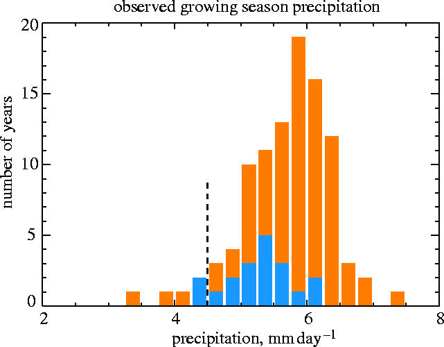
Mean rainfall (mm day⁻¹) during the growing season, as derived from the Climate Research Unit (CRU; University of East Anglia, Norwich, UK) gridded climatology and for the region of latitude 3.75–21.25°N, and longitude 16.875°W–35.625°E. The growing season is defined as the months of July, August and September. The histogram heights given by the orange bars are for the period 1900–1998. The subset of these, given in blue, is the years 1971–1989, which represent an extended period of drought. The vertical dashed line at 4.5 mm day⁻¹ marks the difference between the two extremely dry years in the drought period (years 1983 and 1984), which attracted international action.

The identical statistics from the four twentieth century GCM runs are presented in figure 2. Three distinct inter-model differences are apparent. First, the absolute values vary significantly between the models, with the MRI simulation being particularly dry. Second, the spread of values capturing their estimates of interannual variability is small. However, the third issue, which is of particular interest, is that there is no prediction of the intense and prolonged drought, which began in the early 1970s. This is common to all coupled models we analyse here and suggests that the drought period may not be a consequence of external forcings, but instead is due to natural variability occurring through atmospheric coupling to long time-scale variations in oceanic temperature profiles. We note, however, that the failure of models to reproduce the drought period could also be down to a particular shortcoming common to GCM oceanic descriptions whereby modelled SST change is under-sensitive to alterations in atmospheric CO₂ concentration. A useful set of GCM simulations to create would be long control runs capturing oscillations of the coupled climate system when forced by mean atmospheric greenhouse gas concentrations applicable to period 1971–1989. Comparison with the existing control runs appropriate to pre-industrial atmospheric concentrations would allow an assessment of whether anthropogenic emissions up to that period raised the probability of SST patterns occurring as observed during the two decades of drought. The simulations presented here do, however, fit the current opinion that the causes of the drought are a manifestation of internal variability rather than response to greenhouse forcing. Atmosphere-only GCMs forced by known SSTs alone can reproduce a significant part of the decadal drought signal (Giannini et al. 2003). Such coupled ocean–atmosphere oscillations may be further enhanced over the region by land ecosystem feedbacks, as proposed by Charney (1975) and illustrated with a coupled model by Zeng et al. (1999).

Figure 2.

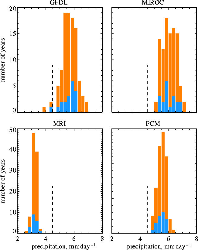
Transient GCM estimates of precipitation for the region, season and years as the observed data given in figure 1 (note different vertical scales). None of the simulations capture the observed mean drying for the period in blue (years 1971–1989).

Figure 3 shows the change in seasonal rainfall predicted by the four GCMs, between the contemporary period and the end of the twenty-first century. Figure 3a and b, give mean monthly rainfall for 1971–1989. We divide the tropical north African region into two latitudinal subareas that we define as ‘Sahel’ (11.25–16.25°N) and ‘Soudan’ (4.75–11.25°N). Figure 3c and d are mean monthly output for 2081–2099 averaged across the three SRES scenarios. In all panels, the black line represents observations for 1971–1989. We selected this period for comparison as it covers a period of drought.

Figure 3.

Mean rainfall by month for the four GCMs. These correspond to an averaging period of 1971–1989 (a,b) and 2081–2099 and averaged across all scenarios (c,d). Two regions are presented (both with the same longitude variation as used in figure 1, but here divided into two bands of ‘the Sahel’ (11.25–16.25°N) and ‘the Soudan’ (4.75–11.25°N)). Each GCM is represented by a different colour, as given in the keys. The black line is the observed data in each region for the period 1971–1989 in all plots.

All the models show a distinct seasonal cycle that qualitatively mimics the observed cycle which is due to the seasonal migration of the inter-tropical convergence zone (ITCZ). We see that the ‘wetter’ models from figure 2 are, generally, wetter for all months. The important result is that there is relatively little change in the monthly model mean predictions between the 1971–1989 and 2081–2099 periods, averaged across these two large areas. However, this may conceal large changes in the spatial patterns and extremes of rainfall.

Table 1 shows the mean percentage change in growing season precipitation for all models and all emission scenarios for 2081–2099 with respect to 1971–1989. For all scenarios, the GFDL model shows a drying, while the other GCMs show a small wetting. There is less consistency across scenarios, but there is a small drying on average (last column).

Table 1.

Mean percentage increases in growing season precipitation in the tropical northern Africa region for each model and scenario combination in 2081–2099 with respect to the observed 1971–1989 climatology.

scenario	GFDL	MIROC	MRI	PCM	mean
A1B	−25.2	11.9	3.5	4.4	−1.4
A2	−33.9	10.3	1.6	1.7	−5.1
B1	−13.8	−2.8	6.9	4.0	−1.4
mean	−24.3	6.5	4.0	3.4	−2.6

All GCM values are ‘nudged’ by removing the mean value for 1971–1989 calculated by that GCM and adding on the observed mean for the same period. There are small percentage decreases for all scenarios, but these are almost entirely down to the GFDL model.

In figure 4, we compare and contrast year-on-year variability across future scenarios (figure 4a) and the four models (figure 4b) for July–September precipitation in the tropical northern Africa. The blue histogram in both panels represents observed rainfall for 1971–1989 with which we nudge all model data so that the 1971–1989 means are the same as those observed. We do this here, because we are interested in capturing future changes in precipitation, rather than overall model performance, which we described in figure 2.

Figure 4.

Mean growing season precipitation, divided into bins of 0.25 mm day⁻¹. Both plots are normalized to a total of 19 years. (a) The coloured lines are averages across all four GCMS for the three SRES scenarios for the period 2081–2099. The black line is the average across all GCMs for their estimates of 1971–1989. All GCM values are ‘nudged’ by removing the mean value for 1971–1989 calculated by that GCM and adding on the observed mean for the same period. The GCMs, therefore, only provide information on the distribution about the mean for each 19 year period and future changes in the mean. (b) The solid coloured lines are averages across all three scenarios for each GCM for 2081–2099. The dashed coloured lines are GCM estimates for 1971–1989. The blue bars and vertical black dashed line plotted in both panels have the same meaning as in figure 1.

In figure 4a, we see that, despite small increases in mean growing season precipitation for three of the models, larger numbers of extreme dry and wet years are expected for all scenarios—especially A1B and A2. Large increases in the number of expected dry years are a concern for agriculture. Inspecting figure 4b, however, we see that although all four models show increases in rainfall extremes (solid lines), much of the increase in dry years comes from the GFDL model, which shows large mean drying. Another issue is the use of 1971–1989 as the climatology period. While this does allow the comparison of future climate changes to contemporary climate, the 1971–1989 period was unusually dry for the twentieth century (figure 1). If this is the consequence of natural variability, as the models suggest (figure 2), and not a forced change in climate, then the nudged anomalies of figure 4 will predict too many dry years. Nevertheless, the models still predict that there will be more dry years in future with respect to their own contemporary climates.

(c) Short time-scale extremes

In §2b, we found that although the four GCMs predict relatively little change in future mean rainfall over tropical northern Africa, they do imply the possibility of significant increases in the number of drought years. In addition, there may be important changes in climate limited to small spatial and temporal scales that do not manifest themselves in monthly mean, area averaged data, but could also damage crop yields. Here, we investigate model predicted changes in gridded daily precipitation and temperature data. These quantities are of direct importance to physiological response, but to date, have rarely been available as diagnostics from large-scale climate models. The IPCC data centre has provided access to new GCM output, where these diagnostics are available.

Figure 5 shows the mean and standard deviation of changes in the number of ‘dry weeks’ in the four GCMs. Rather than choose a real threshold known to cause crop damage, we define a dry week as a 7 day period that falls in the bottom 10% of 7 day periods in the 1971–1989 run of each model. We do this because the models have the tendency to ‘drizzle’ on short time-scales, rather than produce focused storms, and plants experience precipitation via local soil moisture properties that are not well represented. Even so, the change in the percentage of dry weeks below a given threshold will give an indication of how we might expect the frequency of crop damage to change in future.

Figure 5.

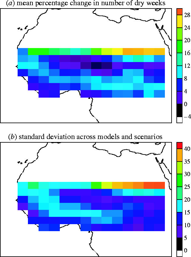
Model predictions of changes in frequency of low rainfall. For each climate model during the period (1971–1989) and for the growing season defined as July–September, we calculate the average daily precipitation threshold below which 10% of all consecutive 7 day periods fall. For all models and all three SRES scenarios, we calculate the percentage changes in occurrence of 7 day periods drier than that threshold for 2081–2099. (a) The mean percentage change across all models and scenarios is plotted, while in (b) the standard deviation across models and scenarios is plotted.

Figure 5a shows future changes in the number of dry weeks during the growing season for tropical northern Africa across all models and scenarios. At almost all points there is an increase in the number of dry weeks, although this pattern shows significant spatial variability. Further, the variance between models is large (see figure 5b). In table 1, the overall mean change across all models and all scenarios for growing season rainfall is small. This implies the larger percentage changes in dry weeks corresponds to fewer but more intense storms in a future climate.

Figure 6 shows the number of days during the 92 day growing season when the mean temperature is greater than 33 °C (a temperature above which cereal crops suffer major physiological damage; Peter Craufurd, personal communication). All the model data are nudged so that mean monthly temperatures during 1971–1989 are the same as those observed (New et al. 2000). Figure 6a shows the number of ‘hot days’ occurring in the models during the 1971–1989 period. Figure 6b shows increases in the number of hot days for most of the tropical northern Africa region. In particular, figure 6 shows hot days in the more populated southern part of the region, where there were none during 1971–1989. Figure 6c shows large inter-model and inter-scenario differences in predicted changes in number of hot days.

Figure 6.

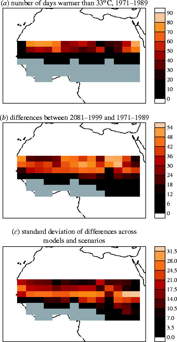
Model predictions of changes in number of ‘hot days’. For each climate model during the period (1971–1989), and for the growing season defined as July–September, we calculate the number of days where the mean temperature is greater than 33 °C. The grey area corresponds to regions, where there are no days greater than this threshold. (a) Model values (averaged across all models), but ‘nudged’ such that the monthly mean values equal those from the Hulme dataset for the period 1971–1989. (b) For all models and all three SRES scenarios, we calculate the changes in number of days greater than 33 °C. (c) The standard deviation across models and scenarios of the change presented in (b).

3. Future recommendations for climate modelling activities

(a) Climate model configuration and diagnostics

Although GCMs have the potential to provide required information on changes in surface climate for determining future crop yields, a key result from this paper is that there are major differences between their projections. This uncertainty makes it currently impossible to provide accurate estimates of the future. There is notable effort at present in extending GCMs to reproduce more facets of the Earth system, including direct coupling to impacts submodels. While this is to be applauded, the analysis presented here highlights that there are still fundamental aspects of climate modelling (e.g. the hydrological cycle) that require refinement and process understanding. Major measurement campaigns operating at present, or about to be initiated (e.g. the African Monsoon Multidisciplinary Analyses) will provide the data needed to constrain model performance for the contemporary period.

Meehl et al. (2000) point out that at current GCM resolutions, process modelling of clouds and precipitation, which directly influences projections of extremes, is heavily parameterized and thus, not described explicitly. High-resolution climate data are needed if biological and hydrological processes are to be adequately represented (see e.g. Mearns et al. 2001). At present, the large gridbox size in GCMs means that sub-grid scale variability is not adequately represented (storms are often simulated as drizzle across a full GCM gridbox), and yet it is exactly this information that is required. A continued push towards ever higher resolution climate models is needed, and increasing computer power will help in this endeavour, provided that appropriate fundamental understanding of process behaviour at the smaller-scale is also available. Uncertainty in model parameterization has been addressed by Murphy et al. (2004) and Stainforth et al. (2005) who present ensembles of model simulations with a range of parameter values, but neither study investigated regional climate impacts. Another possibility is extended use of fine resolution regional climate models (RCMs) ‘nested’ in GCMs for areas of known vulnerability.

This paper discusses the drought period of the 1970s and 1980s, and whether GCMs indicate this was a natural phenomenon. To describe the statistical structure of oscillations in the Earth system that occur over long (decadal) time periods, extended atmosphere–ocean simulations are required. These are frequently undertaken to check the ‘stability’ of climate models at the end of a ‘spin-up’ period, and investigate model variability. Archiving large quantities of model data is becoming easier with the very rapid increase in disk storage size. It has become easier to save higher temporal resolution data (daily rainfall from all GCMs in the IPCC database would enhance the analysis presented here) and to also retain more novel diagnostics that are of relevance to impacts assessments (e.g. predictions of soil moisture content). Further analysis of comprehensive diagnostics could allow investigation of particular aspects of rainfall patterns not considered here, but still of importance to crop yields (e.g. actual start date of the monsoon and sub-seasonal variability).

One issue that has not been addressed in this paper is the potential for direct feedbacks on climate due to changes in vegetation. These could occur if large-scale alternative LUs are introduced as a means to adapt to a changing climate or dwindling resources, or as a response of the natural vegetation to climate change. The potential for the land surface to feedback on the global carbon cycle in response to anthropogenic climatological forcing has already been established (Cox et al. 2000). However, there is also the possibility of a feedback at the regional scale due to changes in surface fluxes of heat and water. Indeed, the focus of §2, the African monsoon, is considered to be especially sensitive to both natural (Zeng et al. 1999) and anthropogenic (Taylor et al. 2002) changes in vegetation. There is little consensus among models of how important these feedbacks are for current climate (Koster et al. 2004), let alone sensitivity to enhanced CO₂ (Gedney et al. 2000). On-going activities in improving soil–vegetation–atmosphere transfer models (including multiple vertical layers capturing canopy variation in vegetation) for impacts purposes may ultimately improve the climate model predictions themselves.

(b) Accessibility to climate information and new routes to impact assessment

Despite concerns raised above regarding the need to include land–atmosphere feedbacks, if an assumption is made that (at least on a very local scale) these are relatively weak, then an initial assessment of future climate change induced adjustment to food security can be achieved by forcing crop models ‘off-line’ with climate model output. This avoids the requirement for those researching food sustainability to carry the overhead of operating full climate models. Combining GCM data with local process understanding of crop yield and phenological behaviour will empower agricultural research scientists to project the future availability of food. But a range of numerical tools are available that have the capacity to allow individual researchers to undertake ‘GCM-like’ simulations without the need for a GCM. These include numerical algorithms that capture GCM output for use by impacts models such as magicc/scengen models (Hulme et al. 2000) and the GCM analogue model (Huntingford & Cox 2000). The latter has been coupled to the land surface scheme of the HadCM3 model (Cox et al. 1998) to create a coupled impacts tool, called IMOGEN (Huntingford et al. 2004). These computationally efficient impact models use GCM-modelled patterns in surface climate to predict a range of possible future climates. These off-line tools could be extended to provide the diagnostics needed for estimating crop yield.

There are already some studies available that strive to estimate change in agricultural yield. For instance, Parry et al. (2004) study present day correlations between known crop yields and temperature and precipitation anomalies during the growing period, and then use these to develop refined estimates based on projections of climate change. More process-based modelling studies linking GCM output with crop growth descriptions that take account of local conditions (such as soil content) are necessary (e.g. Challinor et al. 2005). Continuing this line of analysis, we have considered the frequency of temperature threshold exceedance, but this cannot be related simply to the risk of low crop yield, as the full impact on yield will depend in a nonlinear fashion on the magnitude and timing of these high-temperature events and links to other influences such as planting date and soil type. In the first instance, existing off-line simulations of crop yield that use daily weather data (e.g. Challinor et al. 2004) should be repeated across a range of GCMs to extend our current understanding of where significant changes in the world are likely to occur.

New tools are emerging that capture the balance of different and competing future environmental stresses from local, global and socio-economic pressures. An emerging example of such an integrated assessment is the ‘climate vulnerability index’ (Sullivan & Meigh 2005), an extension of the ‘water poverty index’ (Sullivan 2002; Sullivan et al. 2003) which maps water vulnerability onto local socio-economic statistics, thereby capturing neighbourhood knowledge, but also including a key component representing climatological change. It is recommended that this latter component is calibrated tightly against available GCM data.

McAveny et al. (2001) noted that none of the major intercomparison projects has triggered research into GCM ability to capture extremes, and states ‘very few coupled models have been subjected to any form of systematic extreme event analysis’. Greater involvement of the researchers in the regions under study will result in more testing of model predictions of extremes by exploiting local knowledge and meteorological data.

4. Conclusions

We have analysed climate model projections of change in temperature and rainfall for the tropical northern Africa region corresponding to enriched greenhouse gas concentration futures. Tropical northern Africa is an area of particular vulnerability regarding food security, and any adjustment to surface climate will impact on crop yields. Alterations to rainfall and temperature, including the statistical likelihoods of extremes, are of major importance. General circulation models are the best tools available to provide detailed estimates of projected climate variation that correspond to raised concentrations of greenhouse concentrations in response to fossil fuel burning. They are explicitly designed to operate at the century time-scale and to capture all the major known features of the coupled Earth system. However, this paper demonstrates that such models show significant variation in estimates of rainfall characteristics for even the present tropical northern African climate, and implies that improvement of fundamental representation of the hydrological cycle is needed. Comparison with observed meteorological datasets for the region is a first step. It is noted that three of the models predict a general increase of rainfall, which should be beneficial for crop yield, although simultaneously there are higher numbers of low-rainfall weeks during the growing season. A more robust signal seen in all the GCMs is that there will be a significant increase in the number of very high-temperature days, which could reduce crop yields.

The massive computational requirement of GCMs means that at any individual point, the ‘gridbox’ size is large (typical order 200 km). Many features of importance at the sub-grid scale (e.g. structure of individual storms, influence of local topography) are, therefore, parameterized. To enable rigorous comparison to data, and to allow climate model projections to be of more use for impacts assessment, a significant reduction in spatial scale is required. ‘Nested’ RCMs for the tropical northern African area may fulfil this need, returning a spatial scale down to order 20 km.

As GCM refinement continues the uncertainty in future projections should decrease and more trust will be placed in their capabilities for future planning purposes. Methods of downscaling large-scale diagnostics to the small-scales necessary to assess impacts on agriculture will make GCM output more meaningful. Fine resolution estimates of future weather, including the statistical properties of individual storm events and extreme daily temperature values, provide forcing data to drive crop model simulations and allow estimates of future yields. It is important that researchers in vulnerable regions have access to both crop submodels and model-derived fine resolution gridded driving data of climatological forcings for a range of emission scenarios. This will enable simulations to be made for the countries where food security is a major concern for the future, and will empower such countries to make a full contribution to international negotiations on climate change mitigation based on strong scientific understanding of the potential impacts in those countries.

References

- Brooks N, Huntingford C, Gash J.H.C, Kjellen B, Köhler J, Starkey R, Warren R, Hulme M. Climate stabilisation and ‘dangerous’ climate change: a review of the issues. Climatic Change. 2006 in press. [Google Scholar]
- Challinor A.J, Slingo J.M, Wheeler T.R, Craufurd P.Q, Grimes D.I.F. Towards a combined seasonal weather and crop productivity forecasting system: determination of the working spatial scale. J. Appl. Meteorol. 2003;42:175–192. doi:10.1175/1520-0450(2003)042<0175:TACSWA>2.0.CO;2 [Google Scholar]
- Challinor A.J, Wheeler T.R, Craufurd P.Q, Slingo J.M, Grimes D.I.F. Design and optimization of a large-area process-based model for annual crops. Agric. Forest Meteorol. 2004;124:99–120. doi:10.1016/j.agrformet.2004.01.002 [Google Scholar]
- Challinor A.J, Wheeler T.R, Slingo J.M, Craufurd P.Q, Grimes D.I.F. Simulation of crop yields using ERA-40: limits to skill and nonstationarity in weather–yield relationships. J. Appl. Meteorol. 2005;44:516–531. doi:10.1175/JAM2212.1 [Google Scholar]
- Charney J.G. Dynamics of deserts and drought in the Sahel. Q. J. R. Meteorol. Soc. 1975;101:193–202. doi:10.1256/smsqj.42801 [Google Scholar]
- Cowan I.R. Stomatal behaviour and environment. Adv. Bot. Res. 1977;4:117–128. [Google Scholar]
- Cowan I.R, Farquhar G.D. Stomatal function in relation to leaf metabolism and environment. In: Jennings D.H, editor. Integration of activity in the higher plant. Cambridge University Press; New York: 1977. pp. 471–505. Symposium of the Society for Experimental Biology Vol. 31. [PubMed] [Google Scholar]
- Cox P.M, Huntingford C, Harding R.J. A canopy conductance and photosynthesis model for use in a GCM land surface scheme. J. Hydrol. 1998;213:79–94. doi:10.1016/S0022-1694(98)00203-0 [Google Scholar]
- Cox P.M, Betts R.A, Jones C.D, Spall S.A, Totterdell I.J. Acceleration of global warming due to carbon-cycle feedbacks in a coupled climate model. Nature. 2000;408:184–187. doi: 10.1038/35041539. doi:10.1038/35041539 [DOI] [PubMed] [Google Scholar]
- Cubasch U, Meehl G.A, Boer G.J, Stouffer R.J, Dix M, Noda A, Senior C.A, Raper S, Yap K.S. Projections of future climate change. In: Houghton J.T, Ding Y, Griggs D.J, Noguer M, van der Lind P.J, Dai X, Maskell K, Johnson C.A, editors. Climate change 2001: the scientific basis. Cambridge University Press; Cambridge, UK: 2001. pp. 525–582. Contribution of Working Group 1 to the Third Assessment Report of the IPCC. [Google Scholar]
- Easterling D.R, Meehl G.A, Parmesan C, Changnon S.A, Karl T.R, Mearns L.O. Climate extremes: observations, modeling and impacts. Science. 2000;289:2068–2074. doi: 10.1126/science.289.5487.2068. doi:10.1126/science.289.5487.2068 [DOI] [PubMed] [Google Scholar]
- FAO. World agriculture: towards 2015/2030. In: Bruinsma J, editor. An FAO perspective. Earthscan; London, UK: 2003. p. 432. [Google Scholar]
- Felzer B, Kicklighter D, Melillo J, Wang C, Zhuang Q, Prinn R. Ozone effects on net primary production and carbon sequestration in the conterminous United States using a biogeochemistry. Tellus B. 2004;56:230–248. doi:10.1111/j.1600-0889.2004.00097.x [Google Scholar]
- Folland C.K, et al. Observed climate variability and change. In: Houghton J.T, Ding Y, Griggs D.J, Noguer M, van der Lind P.J, Dai X, Maskell K, Johnson C.A, editors. Climate change 2001: the scientific basis. Cambridge University Press; Cambridge, UK: 2001. pp. 99–181. Contribution of working group 1 to the third assessment report of the IPCC. [Google Scholar]
- Gedney N, Cox P.M, Douville H, Polcher J, Valdes P.J. Characterizing GCM land surface schemes to understand their responses to climate change. J. Climate. 2000;13:3066–3079. doi:10.1175/1520-0442(2000)013<3066:CGLSST>2.0.CO;2 [Google Scholar]
- Giannini A, Saravanan R, Chang P. Oceanic forcing of Sahel rainfall on interannual to interdecadal time scales. Science. 2003;302:1027–1030. doi: 10.1126/science.1089357. doi:10.1126/science.1089357 [DOI] [PubMed] [Google Scholar]
- Gillett N.P, Zwiers F.W, Weaver A.J, Stott P.A. Detection of human influence on sea level pressure. Nature. 2003;422:292–294. doi: 10.1038/nature01487. doi:10.1038/nature01487 [DOI] [PubMed] [Google Scholar]
- Gregory J.M, Huybrechts P, Raper S.C.B. Climatology: threatened loss of the Greenland ice-sheet. Nature. 2004;428:616. doi: 10.1038/428616a. doi:10.1038/428616a [DOI] [PubMed] [Google Scholar]
- Houghton J.T. 3rd edn. Cambridge University Press; Cambridge, UK: 2002. The physics of atmospheres. [Google Scholar]
- Hu Z.Z, Wu Z.H. The intensification and shift of the annual North Atlantic oscillation in a global warming scenario simulation. Tellus. 2004;56:112–124. doi:10.1111/j.1600-0870.2004.00050.x [Google Scholar]
- Hulme M. A 1951–80 global land precipitation climatology for the evaluation of general-circulation models. Climate Dyn. 1992;7:57–72. doi:10.1007/BF00209609 [Google Scholar]
- Hulme M, Wigley T.M.L, Barrow E.M, Raper S.C.B, Centella A, Smith S, Chipanshi A.C. Climatic Research Unit, UEA; Norwich, UK: 2000. Using a climate scenario generator for vulnerability and adoption assessments: Magicc and Scengen version 2.4 workbook; p. 52. [Google Scholar]
- Huntingford C, Cox P.M. An analogue model to derive additional climate change scenarios from existing GCM simulations. Climate Dyn. 2000;16:575–586. doi:10.1007/s003820000067 [Google Scholar]
- Huntingford C, Harris P.P, Gedney N, Cox P.M, Betts R.A, Marengo J.A, Gash J.H.C. Using a GCM analogue model to investigate the potential for Amazonian forest dieback. Theor. Appl. Climatol. 2004;78:177–185. doi:10.1007/s00704-004-0051-x [Google Scholar]
- Jarvis P.G. The interpretation of leaf water potential and stomatal conductance found in canopies in the field. Phil. Trans. R. Soc. B. 1976;273:593–610. [Google Scholar]
- Koster R.D, et al. Regions of strong coupling between soil moisture and precipitation. Science. 2004;305:1138–1140. doi: 10.1126/science.1100217. doi:10.1126/science.1100217 [DOI] [PubMed] [Google Scholar]
- Lomberg B. Cambridge University Press; Cambridge, UK: 2001. The skeptical environmentalist—measuring the real state of the world; p. 515. [Google Scholar]
- Mann M.E, Bradley R.S, Hughes M.K. Global-scale temperature patterns and climate forcing over the past six centuries. Nature. 1998;392:779–787. doi:10.1038/33859 [Google Scholar]
- McAveny B.J, et al. Model evaluation. In: Houghton J.T, Ding Y, Griggs D.J, Noguer M, van der Lind P.J, Dai X, Maskell K, Johnson C.A, editors. Climate change 2001: the scientific basis. Contribution of Working Group 1 to the Third Assessment Report of the IPCC. Cambridge University Press; Cambridge, UK: 2001. pp. 471–523. [Google Scholar]
- Mearns L.O, Easterling W, Hays C, Marx D. Comparison of agricultural impacts of climate change model scenarios. Part I. The uncertainty due to spatial scale. Climatic Change. 2001;51:1–42. doi:10.1023/A:1012297314857 [Google Scholar]
- Meehl G.A, Collins W.D, Boville B.A, Kiehl J.T, Wigley T.M.L, Arblaster J.M. Response of the NCAR climate system model to increased CO2 and the role of physical processes. J. Climate. 2000;13:1879–1898. doi:10.1175/1520-0442(2000)013<1879:ROTNCS>2.0.CO;2 [Google Scholar]
- Murphy J.M, Sexton D.M.H, Barnett D.N, Jones G.S, Webb M.J, Collins M. Quantification of modelling uncertainties in a large ensemble of climate change simulations. Nature. 2004;430:768–772. doi: 10.1038/nature02771. doi:10.1038/nature02771 [DOI] [PubMed] [Google Scholar]
- Nakićenović N, et al. Cambridge University Press; Cambridge, UK: 2000. Emission scenarios. [Google Scholar]
- New M, Hulme M, Jones P. Representing twentieth-century space–time climate variability. Part II. Development of 1901–96 monthly grids of terrestrial surface climate. J. Climate. 2000;13:2217–2238. doi:10.1175/1520-0442(2000)013<2217:RTCSTC>2.0.CO;2 [Google Scholar]
- Øygard R, Vedeld T, Aune J. Noragric; Norway: 1999. Good practices in drylands management; p. 116. See http://www.encapafrica.org/EGSSAA/current_EGSSAA_sector_bibliography/EGSSAA-Ch01-Agric-biblio.htm. [Google Scholar]
- Parry M.L, Rosenzweig C, Iglesias A, Livermore M, Fischer G. Effects of climate change on global food production under SRES emissions and socio-economic scenarios. Global Environ. Change. 2004;14:53–67. doi:10.1016/j.gloenvcha.2003.10.008 [Google Scholar]
- Rahmstorf S, Stocker T.F. Thermohaline circulation: past changes and future surprises? In: Steffen W, et al., editors. Global change and the earth system: a planet under pressure. Springer; Berlin: 2004. pp. 240–241. IGBP global change series. [Google Scholar]
- Stainforth D.A, et al. Uncertainty in predictions of the climate response to rising levels of greenhouse gases. Nature. 2005;433:403–406. doi: 10.1038/nature03301. doi:10.1038/nature03301 [DOI] [PubMed] [Google Scholar]
- Steffen W, et al. Abrupt changes: the Achilles' heels of the Earth System. Environment. 2004;46:8–20. [Google Scholar]
- Stott P.A, Tett S.F.B, Jones G.S, Allen M.R, Mitchell J.F.B, Jenkins G.J. External control of 20th century temperature by natural anthropogenic forcings. Science. 2000;290:2133–2137. doi: 10.1126/science.290.5499.2133. doi:10.1126/science.290.5499.2133 [DOI] [PubMed] [Google Scholar]
- Sullivan C.A. Calculating a water poverty index. World Dev. 2002;30:1195–1210. doi:10.1016/S0305-750X(02)00035-9 [Google Scholar]
- Sullivan C.A, Meigh J.R. Targeting attention on local vulnerabilities using a integrated index approach: the example of the Climate Vulnerability Index. Water Sci. Technol. 2005;51:69–78. [PubMed] [Google Scholar]
- Sullivan C.A, et al. The water poverty index: development and application at the community scale. Nat. Resour. Forum. 2003;27:189–199. doi:10.1111/1477-8947.00054 [Google Scholar]
- Taylor C.M, Lambin E.F, Stephenne N, Harding R.J, Essery R.L.H. The influence of land use change on climate in the Sahel. J. Climate. 2002;15:3615–3629. doi:10.1175/1520-0442(2002)015<3615:TIOLUC>2.0.CO;2 [Google Scholar]
- Wheeler T.R, Craufurd P.Q, Ellis R.H, Porter J.R, Vara Prasad P.V. Temperature variability and the yield of annual crops. Agric. Ecosyst. Environ. 2000;82:159–167. doi:10.1016/S0167-8809(00)00224-3 [Google Scholar]
- Wright G.C, Hubick K.T, Farquhar G.D. Physiological analysis of peanut cultivar response to timing and duration of drought stress. Austr. J. Agric. Res. 1991;42:453–470. doi:10.1071/AR9910453 [Google Scholar]
- Zeng N, Neelin J.D, Lau K.M, Tucker C.J. Enhancement of interdecadal climate variability in the Sahel by vegetation interaction. Science. 1999;286:1537–1540. doi: 10.1126/science.286.5444.1537. doi:10.1126/science.286.5444.1537 [DOI] [PubMed] [Google Scholar]