Simultaneous Fine Mapping of Multiple Closely Linked Quantitative Trait Loci Using Combined Linkage Disequilibrium and Linkage With a General Pedigree

Abstract

Within a small region (e.g., <10 cM), there can be multiple quantitative trait loci (QTL) underlying phenotypes of a trait. Simultaneous fine mapping of closely linked QTL needs an efficient tool to remove confounded shade effects among QTL within such a small region. We propose a variance component method using combined linkage disequilibrium (LD) and linkage information and a reversible jump Markov chain Monte Carlo (MCMC) sampling for model selection. QTL identity-by-descent (IBD) coefficients between individuals are estimated by a hybrid MCMC combining the random walk and the meiosis Gibbs sampler. These coefficients are used in a mixed linear model and an empirical Bayesian procedure combines residual maximum likelihood (REML) to estimate QTL effects and a reversible jump MCMC that samples the number of QTL and the posterior QTL intensities across the tested region. Note that two MCMC processes are used, i.e., an (internal) MCMC for IBD estimation and an (external) MCMC for model selection. In a simulation study, the use of the multiple-QTL model clearly removes the shade effects between three closely linked QTL located at 1.125, 3.875, and 7.875 cM across the region of 10 cM, using 40 markers at 0.25-cM intervals. It is shown that the use of combined LD and linkage information gives much more useful information compared to using linkage information alone for both single- and multiple-QTL analyses. When using a lower marker density (11 markers at 1-cM intervals), the signal of the second QTL can disappear. Extreme values of past effective size (resulting in extreme levels of LD) decrease the mapping accuracy.

THE information from genetic markers has been a valuable resource to detect quantitative trait loci (QTL) in natural, outbred, or experimental populations. The inheritance state of markers has been used to detect existence of quantitative trait variation associated with a putative QTL by using a pedigree-based linkage mapping (Lander and Botstein 1989; Haley and Knott 1992; Andersson et al. 1994; Georges et al. 1995). The use of closely linked markers allows also use of linkage disequilibrium (LD) information and positioning of a QTL within a few centimorgans, i.e., fine mapping (Riquet et al. 1999; Meuwissen and Goddard 2000; Farnir et al. 2002; Grisart et al. 2002; Meuwissen et al. 2002; Perez-Enciso 2003).

In some cases, there may be multiple QTL underlying phenotypes of a trait within a small region (<10 cM). The effects of closely linked QTL can be easily confounded, which may negatively affect precision and accuracy of mapping of each QTL. Multiple QTL in such a small region may be considered as a single QTL; therefore the confidence interval covers all of the region. This makes fine mapping of each QTL impossible. The question is how easily multiple QTL within a small region can be accurately mapped.

Shade effects of neighboring QTL (e.g., ghost QTL) have been discussed for linkage mapping by Haley and Knott (1992) and Martinez and Curnow (1992). Jansen (1993) and Zeng (1993) have proposed a combined method of interval mapping and multiple regression on marker genotypes for mapping multiple QTL simultaneously. In the method, the effects in each putative position are sequentially estimated, conditional on cofactors, i.e., selected markers associated with significant QTL and linked or unlinked to the tested putative QTL position. Due to using cofactors, the effects in a putative position are more accurately estimated, resulting in an improvement of QTL mapping. A decision should be made on which markers should be selected as cofactors and how many cofactors should be simultaneously used, which is a model selection problem.

Model selection strategies have been developed and applied for this problem in gene mapping (Broman and Speed 2002; Sillanpaa and Corander 2002). Stepwise selection (Jansen 1993; Kao et al. 1999; Basten et al. 2000) is a standard model selection technique where the Akaike information criterion (Akaike 1969) or Bayesian information criterion (Schwarz 1978) can be used to correct the model likelihood for the number of parameters fitted. Randomized approaches such as Markov chain Monte Carlo (MCMC) or genetic algorithms have been proposed to find an optimal model (Satagopan et al. 1996; Sillanpaa and Arjas 1998; Calborg et al. 2000; Yi and Xu 2000; Nakamichi et al. 2001; Meuwissen and Goddard 2004).

Green (1995) proposed a reversible jump MCMC that allows the Markov chain to surface state space across different model dimensions according to the correct posterior distribution. This is a generalization of Metropolis–Hastings methods (Metropolis et al. 1953; Hastings 1970) dealing with model selection problems. This technique has been used in multiple-QTL analysis to estimate the number of QTL and their positions in linkage mapping (Heath 1997; Sillanpaa and Arjas 1998, 1999; Lee and Thomas 2000; Yi and Xu 2000; Yi et al. 2003).

In this article, we propose the use of a reversible jump MCMC in a variance component approach using combined LD and linkage (LDL) information to investigate multiple-QTL mapping in a small region. The use of populationwide LD can give critical information about different identity-by-descent (IBD) probabilities in different chromosome segments where typically the size of a segment can be ≪1 cM. We hypothesize that it should be possible to simultaneously map multiple closely linked QTL with a proper model selection approach such as a reversible jump MCMC. The aim of this study is to investigate by simulation the performance of LDL mapping of closely linked multiple QTL within a small region.

MATERIALS AND METHODS

Simulation study:

One hundred generations of a historical population with effective size of 100 were simulated for 40 markers and three QTL in a 10-cM region. No pedigree was recorded for this historical population. The markers are evenly spaced every 0.25 cM and the QTL are positioned at 1.125, 3.875, and 7.875 cM from the first marker. In each generation, the number of male and female parents was 50 and their alleles were transmitted to descendants on the basis of Mendelian segregation using the gene-dropping method (MacCluer et al. 1986). Parents were randomly mated with a total of two offspring for each of 50 mating pairs.

The number of base alleles in each marker locus was four and starting allele frequencies were all at 0.25. The marker alleles were mutated at a rate of 4 × 10⁻⁴/generation (Dallas 1992; Weber and Wong 1993; Ellegren 1995). Therefore, this historical population would have an equilibrium distribution of alleles in all marker loci and LD between the QTL and closely flanking markers.

For each QTL, one of the base alleles surviving with a frequency (π) of >0.1 and <0.9 was randomly chosen and treated as favorable with additive effect q and nonadditive effect d compared to other QTL alleles in generation 100. The magnitudes of q and d were determined from and with fixed variances of , and 6 and , and 3 for the first, second, and last QTL. Pedigree, marker genotypes, and phenotypic values were assumed known only for generations 100 and 101 each with 100 animals. Phenotypes were simulated as

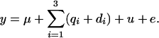The mean of population (μ) was 100, values for were drawn from with , where A ignored the ancestral relationships beyond the known pedigree, and values for were from with . On the basis of this simulation model, we estimated positions of multiple QTL for 40 replicates.

Mixed linear model:

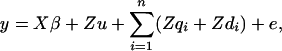
A vector of phenotypic observations is written as a linear function of fixed effects, a polygenic term representing the sum of other unidentified additive genetic effects, the additive and nonadditive effects due to n QTL and residuals. It is assumed that there is no epistatic interaction between QTL. The model can be written as

(1)

where y is a vector of observations on the trait of interest, β is a vector of fixed effects, is a vector of random polygenic effects for each animal, and are a vector of additive and nonadditive random effects due to the putative QTL, and e are residuals. Note that usually is the number of animals in the pedigree. The random effects (u, , , and e) are assumed to be normally distributed with mean zero and variance , , , and , where A is a numerator relationship matrix, and are an additive and nonadditive genotype relationship matrix at the ith putative QTL position, and I is a -order identity matrix. X and are incidence matrices for the effects and u, and , respectively. The associated variance–covariance matrix (V) of all observations given pedigree and marker genotypes is modeled as

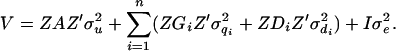(2)

The LDL-based IBD distribution and covariance structure among chromosome segments or haplotypes are accommodated in the matrix G and D used in a variance component approach that treats QTL as random effects. Due to its generality and robustness, the variance component approach has been widely used in mapping studies (George et al. 2000; Yi and Xu 2000; Lund et al. 2003; Perez-Enciso 2003). For G and D, a sampler combining the random walk approach (Sobel and Lange 1996) and the meiosis Gibbs sampler (Thompson and Heath 1999) is used, which is robust and efficient especially for a complex pedigree, many markers, and missing genotypes (Lee et al. 2005). These G and D are then incorporated as known quantities into the QTL model selection in a two-step approach (George et al. 2000). The QTL model is defined by the number of QTL and their positions, which are sampled from a proposal distribution. For a given QTL model, residual maximum-likelihood (REML) estimates for the model parameters are obtained, which is an empirical Bayesian approach (Casella 2001). The proposed variables and model parameters are accepted or rejected, according to the acceptance ratio from a reversible jump MCMC. The posterior QTL density is derived from 10,000 cycles of reversible jump (RJ)MCMC. Hence, a REML procedure is used nested within a Bayesian RJMCMC. Details of this approach follow.

MCMC approach estimating IBD probabilities G and D given marker data:

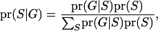
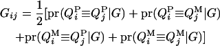
IBD coefficients between individuals can be estimated according to the pattern of inheritance states (S). The probability of one configuration of S given observed marker data is

(3)

where represents the observed marker data, pr() is the prior probability of the segregation state, pr(|) is the probability of the observed marker data given the , and the denominator is summed over the probabilities of all possible configurations of . Since the computation of the denominator is infeasible in a general pedigree with many markers, a MCMC approach is used to surface all possible S according to the posterior distribution.

Sampling schemes for segregation states:

In a MCMC method, updated variables for segregation states are proposed on the basis of an approximate distribution and acceptance for the updated variables is determined on the basis of the Metropolis–Hastings algorithm (Metropolis et al. 1953; Hastings 1970), which gives the correct equilibrium distribution of segregation states. In a Gibbs sampler (a special case of MCMC), updated variables are always accepted because they are sampled on the basis of the correct distribution.

In the MCMC process used in this study, the meiosis Gibbs sampler (Thompson and Heath 1999) is first applied to all loci for every individual. During the meiosis sampler, potential reducible sites can be found where transition probabilities from a current state to other states are zero. After one cycle of the meiosis sampler, the random-walk approach (Sobel and Lange 1996) is carried out for proposing segregation states where the size and direction are randomly determined. If proposed variables include any potentially reducible sites detected in the meiosis sampler, proposal variables are accepted as new variables with a Metropolis acceptance probability (4). This combined sampler is computationally efficient and has a better mixing property:

(4)

(for more details, see Lee et al. 2005).

Haplotype reconstruction:

Since LD-based IBD probabilities are derived from haplotype similarity between unrelated base animals, ordered genotypes for base animals are required to reconstruct haplotypes. The ordered genotypes can be sampled on the basis of the distribution of compatible allele assignments to founder genes that are consistent with the sampled segregation states (Sobel and Lange 1996). When this procedure is implemented for multiple marker loci, haplotypes for base animals are established. This procedure is performed in each sampling round.

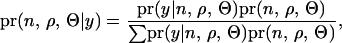
QTL allelic IBD coefficients based on LD and linkage:

Given the sampled segregation state and haplotypes, it is possible to estimate QTL allelic IBD coefficients on the basis of LD and linkage. Sampled haplotypes for unrelated founders in the pedigree are used to estimate LD-based IBD probabilities between them, using an approximated coalescence method (Meuwissen and Goddard 2001). This method assumes past effective size and number of generations since base population known. Sampled segregation states at multiple marker loci for descendents are used to estimate linkage-based IBD probabilities between haplotypes of relatives. Therefore, IBD probabilities between all haplotypes can be estimated on the basis of joint information from LD and linkage. In this study, the IBD probabilities are estimated at the middle point of each marker bracket. There are four IBD probabilities between any pair of individuals i and j in the pedigree for a given putative QTL position (Liu et al. 2002). They are , , , and , the probability of paternal (P) or maternal (M) QTL allele of individual i being IBD to the paternal (P) or maternal (M) allele of individual j, given marker genotypes.

From the probabilities, the additive genotype coefficient between animals i and j at the QTL is

and the dominance relationship coefficient between animals i and j at the QTL is

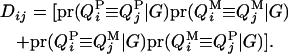The brief summary of the sampling procedure to estimate G and D:

Do 1 ∼ N cycles

• Sample segregation states using the combined MCMC sampler

• Sample haplotypes for unrelated founders

• IBD estimation based on sampled haplotypes and segregation states

• Construct G based on IBD coefficients

• Construct D based on IBD coefficients

End do

• Average G and D over N cycles

We used 100 cycles for the sampling. In each cycle, the meiosis Gibbs sampler was applied to all meiosis and then there were thousands of random-walk samples following.

Reversible jump MCMC for simultaneous mapping of multiple QTL:

The number of QTL (n), the position of each QTL (, i = 1 ∼ n), and the model parameters () are to be estimated for the model (1). Note that n ranges from 0 to the number of marker brackets as only the middle point of each marker bracket is investigated. The probability of estimated parameters given observed phenotypes is

(5)

where is the likelihood of the observed phenotypes given the estimated parameters, is the joint prior probability of the estimated parameters, and the denominator is summed over the probabilities of all possible parameter states. If the computation of the denominator is infeasible, a MCMC approach can be an efficient tool for this problem.

When varying the number of QTL, the model dimension (the number of parameters in the model) is changed. A Metropolis–Hastings sampler cannot infer the correct distribution unless the model dimension is fixed. However, a reversible jump MCMC (Green 1995) allows the Markov chain to jump across states of different dimension and can surface all possible states between different dimensions according to the posterior distribution (Sorensen and Gianola 2002).

For the move of the Markov chain within a fixed model dimension (the number of QTL is unchanged), each QTL position in the current model is subsequently updated with a Metropolis mechanism as in Sillanpaa and Arjas (1998) and Yi and Xu (2000). For the ith QTL in the model, is proposed from a uniform distribution over unoccupied marker brackets. For a given QTL model (i.e., a proposal for and n), REML estimates for the model parameters () are explicitly determined using an average information (AI) algorithm (see Lee and Van der Werf 2006). Note that with the REML estimates, individual level parameters (1) are automatically determined. This procedure is different from conventional MCMC where the model parameters are proposed with the proposal distribution. Assuming that the priors of have a noninformative flat distribution, the proposal is accepted with probability

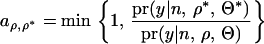(6)

For the move of the Markov chain across different model dimensions (the number of QTL is changed), a new QTL is added (n + 1) or deleted (n − 1) with a proposal probability. A new QTL with position () is uniformly sampled from all unoccupied putative positions across the region. The proposal is accepted with probability

(7)

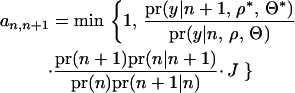
A QTL is deleted from the model by randomly choosing among the QTL. The proposal is accepted with probability

(8)

In (7) and (8), the first term in the right-hand side is the likelihood ratio of proposal parameters over current parameters, and the second term consists of the prior ratio and the proposal ratio. The prior of the number of QTL [e.g., pr(n)] has a Poisson distribution with mean = 1, assuming that the tested region has a single QTL, pr(n*|n) is a proposal probability of changing the number of QTL in the model from n to n*, and J is the Jacobian of the transformation function probability from the current model to the other. Because adding or deleting a QTL in the method is the identity transformation, J = 1 (Sillanpaa and Arjas 1998; Yi and Xu 2000; Jannink and Fernando 2004). The acceptance ratio is formally derived in the appendix and empirically checked (see discussion).

RESULTS

Single- and multiple-QTL analysis:

Likelihood ratio () from a single-QTL analysis and Bayesian posterior QTL intensity from a reversible jump MCMC (as a multiple-QTL analysis) at each putative QTL position averaged over replicates are illustrated in Figure 1. The values of the posterior QTL intensities from the multiple-QTL analysis are clearly highest at the true QTL positions, compared to the neighboring regions. The three QTL are clearly distinguishable and mapped at the correct positions. However, the likelihood-ratio (LR) values from the single-QTL analysis are constantly high across the first and second QTL region. The LR profile across the region between the second and third QTL is also less distinctive, compared to the profile from the multiple-QTL analysis. This shows that the reversible jump MCMC can accurately map the three QTL in such a small region, whereas accurate fine mapping is not feasible by using a single-QTL method.

Figure 1.—

Likelihood ratio () from single-QTL analysis (A) and Bayesian posterior QTL intensity from multiple-QTL analysis (B) averaged over 40 replicates. The vertical bars indicate empirical standard error. Triangles show the true QTL positions.

Multiple-QTL analysis with or without D:

Figure 2 compares the posterior QTL intensity from the multiple-QTL analysis with using D (Figure 2A) and that without using D (Figure 2B). The QTL intensity on the true QTL is higher with D (0.19, 0.16, and 0.14) than on those without D (0.13, 0.09, and 0.11 for the first, second, and third QTL). The curve is more clearly peaked at the correct QTL position when using D, indicating that using D helps map QTL more accurately in the case of the dominance mode.

Figure 2.—

Posterior QTL intensity from multiple-QTL analysis with fitting dominance (A) and without fitting dominance (B) averaged over 40 replicates. The vertical bars indicate empirical standard error. Triangles show the true QTL positions.

LDL vs. linkage information only:

The LR and the posterior QTL intensity based on LDL information are compared with those based on linkage information only in Figure 3. The LR curve is much lower and flatter when using linkage information alone, compared to using LDL information (Figure 3A). The curve of the QTL intensity in the multiple-QTL analysis also shows that linkage information alone does not catch any QTL signal while LDL information gives substantial evidence for the true QTL positions (Figure 3B). It should be noted that the LR and QTL intensity are from analyses without using D for a fair comparison because there is little or no information about dominance relationships for linkage information alone. If D is used, the advantage of LDL information increases over linkage information only (see Figure 2A).

Figure 3.—

Likelihood ratio (LR) and posterior QTL intensity from single- (A) and multiple- (B) QTL analyses based on combined LD and linkage (shaded line) and linkage only (solid thin line). Dominance is not considered for a fair comparison. The vertical bars indicate empirical standard error. Triangles show the true QTL positions.

Effect of marker density:

The profiles of the QTL intensity from multiple-QTL analysis with a marker spacing of 0.25 and 1 cM are compared for a region of 10 cM in Figure 4. Note that the intensity value is estimated at the middle of each marker bracket. When using a marker spacing of 1 cM, the QTL intensity values are constantly high across the region between the first and the second QTL. This makes it impossible to simultaneously map all the QTL although the region can be roughly detected. This is different from when using a marker spacing of 0.25 cM where the intensity value is highly peaked at each true QTL position. With a marker spacing of 1 cM, although the QTL intensity increases at the third QTL, it is not clearly peaked compared to a marker spacing of 0.25 cM.

Figure 4.—

Posterior QTL intensity from multiple-QTL analysis with dense markers (solid thin line) and sparse markers (shaded line). The vertical bars indicate empirical standard error. Triangles show the true QTL positions.

Past effective size in relation to levels of LD:

Levels of LD vary with different values of past effective sizes. Figure 5 shows the QTL intensities averaged over replicates when effective sizes of 10, 100, 400, and 2000 were simulated for 10, 100, 400, and 2000 generations, respectively (the number of generations was equal to the effective size so that a similar population equilibrium was achieved). The intensity values are lower and flatter with the extreme values of effective size (e.g., = 10 or 2000), compared to those with the intermediate values of effective size (e.g., = 100 or 400). The expected levels of LD of chromosome segments given the past effective size are E(LD) = (Sved 1971) where is the past effective size and c is the recombination rate of the chromosome segment. The levels of LD can be defined here as the probability of the chromosome segment being IBD when two random haplotypes are taken from the population (Hayes et al. 2003). For the marker interval used in the simulated data, the expected levels of LD are 0.9, 0.5, 0.2, and 0.05 for N_e = 10, 100, 400, and 2000, respectively. This shows that N_e = 10 or 2000 results in extreme values of LD (0.9 or 0.05) and the mapping accuracy decreases.

Figure 5.—

Posterior QTL intensity from multiple-QTL analysis averaged over 20 replicates with effective sizes of 10 (A), 100 (B), 400 (C), and 2000 (D).

Estimation of the number of QTL and variance components:

Figure 6 shows the histogram of estimated QTL number from 40 replicates. Each estimated value is the average of sampled values of all RJMCMC rounds in each replicate. The distribution coincides with the true value (n = 3) with a small standard error. Estimated values of variance components are also shown to be accurate (Figure 7). The distribution of estimated polygenic and residual variances from 40 replicates shows the highest density at the true value ( = 20 and = 50) (Figure 7, A and B). Although the distribution of estimated additive and dominance QTL variance is upwardly skewed, the mode of the distribution coincides with the true value ( + + = 24, and ) (Figure 7, C and D).

Figure 6.—

Histogram of estimated QTL number for 40 replicates. The true value is 3.

Figure 7.—

Histogram of estimated variance components for 40 replicates. The true values are 20, 50, 24, and 12 for polygenic, residual, additive QTL, and dominance variances.

DISCUSSION

In this study, we investigated the performance of simultaneous fine mapping of closely linked QTL that each had different and relatively small effects (the heritabilities of the first, second, and third QTL were = 0.094, = 0.076, and = 0.057, and the ratios of dominance variance over phenotypic variance were = 0.047, = 0.038, and = 0.028). A multiple-QTL analysis using a reversible jump MCMC could simultaneously position every QTL within a reasonably fine region with 200 genotyped and phenotyped individuals. However, a single-QTL analysis could not remove shade effects between closely linked QTL. The multiple-QTL analysis with dominance relationship matrices improved the mapping accuracy and resolution.

The use of linkage information alone gave a poorer mapping resolution compared to using LDL information. This was because such a small region (10 cM) is not likely to have sufficient recombination from the pedigree of two generations, explaining lower and flatter LR and QTL intensity values from the analyses based on only linkage information. This result agreed with that of Lee and Van der Werf (2005).

When a marker spacing is not dense enough, IBD information from variation in small segments will not contribute to the analyses. This is probably why the second QTL was not clearly distinguishable with a marker spacing of 1 cM while the signal at all the QTL was clearly shown with a marker spacing of 0.25 cM. Optimal marker spacing might depend on the LD in the population. With very small past effective size (N_e = 10) resulting in E(LD) = 0.9 between flanking markers, the mapping resolution was decreased. This was expected because 400 haplotypes used for mapping QTL were descended from only a few founder haplotypes. This made haplotype homozygosity very high, which is not useful for mapping. With very large past effective size (e.g., N_e = 2000), resulting in E(LD) = 0.05, the mapping resolution was also decreased. This was because there were too few common haplotypes with a marker interval of 0.25 cM. If marker density increases, the number of common haplotypes can be increased (i.e., high level of LD), which will give more useful information for mapping of QTL.

In our method, model parameters (Θ) were not sampled from their proposal distributions but the most likely parameter values were determined by REML for a given model defined by the number (n) and location (ρ) of QTL. Using estimates rather than sampled values for some parameters is known as an empirical Bayesian approach (see, e.g., Casella 2001). This differs from the full Bayesian approach where in an MCMC algorithm all model parameters are sampled conditional on data and other parameters. Hence, the posterior distributions for the model parameters might differ somewhat from those of a full Bayesian approach.

The empirical Bayesian approach likely has an efficiency advantage because for sampling values for n and ρ no time is wasted through staying with less likely values of Θ and estimates converge more quickly compared to the full Bayesian approach. It is unlikely that much information is lost in this empirical Bayesian approach because parameters in Θ have smooth distributions and it is not likely that less likely values have critical information. Casella (2001) discussed the empirical Bayesian procedure where in an iterative procedure maximum-likelihood estimates (MLEs) were obtained for hyperparameters in a hierarchical model and other parameters were sampled conditional on these MLEs. He showed that this procedure can be statistically justified by showing that it implies an EM algorithm. In our approach, REML estimates for Θ and the likelihood of the data are explicitly estimated for each model and used in the RJMCMC to get the posterior QTL density across model dimensions. The justification for our procedure is given in the appendix, showing that the acceptance ratios for n and ρ do not depend on conditional distributions for Θ, and hence acceptance ratios used are not different from that in a full Bayesian approach.

We checked the validity of this approach empirically through an analysis without phenotypic data (500,000 rounds), following the suggestion by Jannink and Fernando (2004) and Sillanpaa et al. (2004). In this case, = 1 for all models; therefore, the posterior distribution of the QTL number and their positions should be the same as the prior distribution. Note that the prior for the QTL position was a uniform distribution (see Equation 6) and that for the QTL number was a Poisson distribution with mean (see Equation 7). After 50,000 RJMCMC rounds, the posterior of the QTL position was a uniform distribution, and the posterior of the QTL number was a Poisson distribution with . This implies that the acceptance ratio used in the RJMCMC was correct.

Although, for estimating the number of QTL (n), we used a prior of Poisson distribution with mean , the posterior QTL intensities were substantially higher at all three QTL, and the estimated QTL number was unbiased and accurate (Figure 6). This agreed with previous studies (Yi et al. 2003; Jannink and Fernando 2004; Sillanpaa et al. 2004) that estimates of QTL number were robust against prior values.

The distribution of the estimated variance components from 40 replicates was upwardly skewed and wide especially for additive QTL variance although the mode of the distribution coincided with the true values. This is probably due to the fact that 200 records used in the analyses are not sufficient to (very) accurately estimate variance components. However, the estimated number of QTL and their positions were estimated very accurately with 200 records.

In analyses with linkage information alone, with lower marker density (1-cM intervals), and with alternative past effective sizes, we used true haplotypes instead of sampled haplotypes in the MCMC, as the latter is very time consuming. The results with true and sampled haplotypes were very similar. This agreed with Morris et al. (2004) and Lee and Van der Werf (2005) when using complete genotypes.

Interaction between QTL (epistasis) may be important in multiple-QTL mapping but has been ignored in this study. Epistasis can be considered by working out the appropriate Hadamard products of haplotype (gamete) relationship matrices whose levels are two times the number of individuals. Further investigation on fine mapping of epistasis QTL would be desirable.

APPENDIX

Proving the validity of the empirical Bayesian procedure:

In this method, we obtain a REML estimate of Θ with (RJ)MCMC rather than sampling Θ from proposal distributions, which would be the case in a full Bayesian approach. We show here that the proposal probabilities with REML estimates are not omitted but canceled out from the acceptance ratios used in the full Bayesian approach.

Metropolis–Hastings ratio for QTL position:

In a full Bayesian procedure the acceptance ratio for QTL position given a fixed number of QTL is

with all symbols defined in the text (see Reversible jump MCMC for simultaneous mapping of multiple QTL). The first term is the posterior density consisting of the likelihood and the prior, and the second term is the proposal probability of ρ. In our approach, Θ is always determined by REML with . The equation can be rewritten as

The prior and the proposal probability of QTL positions are a uniform distribution; therefore, they can cancel out. The acceptance ratio is therefore simplified to Equation 6.

RJMCMC probability for QTL birth:

The original acceptance ratio for a QTL birth is

The first term is the posterior density consisting of the likelihood and the prior, and the second term is the proposal probability of adding or deleting a QTL from the model. When deleting a QTL from the model, one QTL is randomly selected with a probability of (n + 1)⁻¹, and the parameters involved in the selected QTL are removed from the model. REML estimates of the model parameters given the reduced number of QTL and their positions are determined with . When adding a QTL to the model, is used with its prior probability (Jannink and Fernando 2004), and REML estimates of the model parameters given the increased number of QTL and positions are determined with . The equation can be rewritten as

Following Jannink and Fernando (2004),

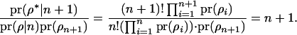This simplifies the equation for to Equation 7. The acceptance ratio for QTL death (Equation 8) can be derived in a similar manner.

References

- Akaike, H., 1969. Fitting autoregressive models for prediction. Ann. Inst. Stat. Math. 21: 243–247. [Google Scholar]
- Andersson, L., C. S. Haley, H. Ellegren, S. A. Knott, M. Johansson et al., 1994. Genetic mapping of quantitative trait loci for growth and fatness in pigs. Science 263: 1771–1774. [DOI] [PubMed] [Google Scholar]
- Basten, C. J., B. S. Weir and Z-B. Zeng, 2000. QTL Cartographer, Version 1.14. North Carolina State University, Raleigh, NC.
- Broman, K. W., and T. P. Speed, 2002. A model selection approach for identification of quantitative trait loci in experimental crosses. J. R. Stat. Soc. B 64: 641–656. [DOI] [PMC free article] [PubMed] [Google Scholar]
- Calborg, O., L. Andersson and B. P. Kinghorn, 2000. The use of a genetic algorithm for simultaneous mapping of multiple interacting quantitative trait loci. Genetics 155: 2003–2010. [DOI] [PMC free article] [PubMed] [Google Scholar]
- Casella, G., 2001. Empirical Bayes Gibbs sampling. Biostatistics 2: 485–500. [DOI] [PubMed] [Google Scholar]
- Dallas, J. F., 1992. Estimation of microsatellite mutation rates in recombinant inbred strains of mouse. Mamm. Genome 3: 452–456. [DOI] [PubMed] [Google Scholar]
- Ellegren, H., 1995. Mutation rates at porcine microsatellite loci. Mamm. Genome 6: 376–377. [DOI] [PubMed] [Google Scholar]
- Farnir, F., B. Grisart, W. Coppieters, J. Riquet, P. Berzi et al., 2002. Simultaneous mining of linkage and linkage disequilibrium to fine map quantitative trait loci in outbred half-sib pedigrees: revisiting the location of a quantitative trait locus with major effect on milk production on bovine chromosome 14. Genetics 161: 275–287. [DOI] [PMC free article] [PubMed] [Google Scholar]
- George, A. W., P. M. Visscher and C. S. Haley, 2000. Mapping quantitative trait loci in complex pedigrees: a two-step variance component approach. Genetics 156: 2081–2092. [DOI] [PMC free article] [PubMed] [Google Scholar]
- Georges, M., D. Nielsen, M. Mackinnon, A. Mishra, R. Okimoto et al., 1995. Mapping quantitative trait loci controlling milk production in dairy cattle by exploiting progeny testing. Genetics 139: 907–920. [DOI] [PMC free article] [PubMed] [Google Scholar]
- Green, P., 1995. Reversible jump Markov chain Monte Carlo computation and Bayesian model determination. Biometrika 82: 711–732. [Google Scholar]
- Grisart, B., W. Coppieters, F. Farnir, L. Karim, L. Ford et al., 2002. Positional candidate cloning of a QTL in dairy cattle: identification of a missense mutation in the bovine dgat1 gene with major effect on milk yield and composition. Genome Res. 12: 222–231. [DOI] [PubMed] [Google Scholar]
- Haley, C. S., and S. A. Knott, 1992. A simple regression method for mapping quantitative trait loci in line crosses using flanking markers. Heredity 69: 315–324. [DOI] [PubMed] [Google Scholar]
- Hastings, W. K., 1970. Monte Carlo sampling methods using Markov chains and their applications. Biometrika 57: 97–109. [Google Scholar]
- Hayes, B. J., P. M. Visscher, H. C. McPartlan and M. E. Goddard, 2003. Novel multilocus measure of linkage disequilibrium to estimate past effective population size. Genome Res. 13: 635–643. [DOI] [PMC free article] [PubMed] [Google Scholar]
- Heath, S. C., 1997. Markov chain Monte Carlo segregation and linkage analysis for oligogenic models. Am. J. Hum. Genet. 61: 748–760. [DOI] [PMC free article] [PubMed] [Google Scholar]
- Jannink, J.-L., and R. L. Fernando, 2004. On the Metropolis–Hastings acceptance probability to add or drop a quantitative trait locus in Markov chain Monte Carlo-based Bayesian analyses. Genetics 166: 641–643. [DOI] [PMC free article] [PubMed] [Google Scholar]
- Jansen, R. C., 1993. Interval mapping of multiple quantitative trait loci. Genetics 135: 205–211. [DOI] [PMC free article] [PubMed] [Google Scholar]
- Kao, C.-H., Z-B. Zeng and R. D. Teasdale, 1999. Multiple interval mapping for quantitative trait loci. Genetics 152: 1203–1216. [DOI] [PMC free article] [PubMed] [Google Scholar]
- Lander, E. S., and D. Botstein, 1989. Mapping Mendelian factors underlying quantitative traits using RFLP linkage maps. Genetics 121: 185–199. [DOI] [PMC free article] [PubMed] [Google Scholar]
- Lee, J. K., and D. C. Thomas, 2000. Performance of Markov chain Monte Carlo approaches for mapping genes in oligogenetic models with an unknown number of loci. Am. J. Hum. Genet. 67: 1232–1250. [DOI] [PMC free article] [PubMed] [Google Scholar]
- Lee, S. H., and J. H. J. Van der Werf, 2005. The role of pedigree information in combined linkage disequilibrium and linkage mapping of quantitative trait loci in a general complex pedigree. Genetics 169: 455–466. [DOI] [PMC free article] [PubMed] [Google Scholar]
- Lee, S. H., and J. H. J. Van der Werf, 2006. An efficient variance component approach implementing an average information REML suitable for combined ld and linkage mapping with a general complex pedigree. Genet. Sel. Evol. 38: 25–43. [DOI] [PMC free article] [PubMed] [Google Scholar]
- Lee, S. H., J. H. Van der Werf and B. Tier, 2005. Combining the meiosis Gibbs sampler with the random walk approach for linkage and association studies with a general complex pedigree and multimarker loci. Genetics 171: 2063–2072. [DOI] [PMC free article] [PubMed] [Google Scholar]
- Liu, Y., G. B. Jansen and C. Y. Lin, 2002. The covariance between relatives conditional on genetic markers. Genet. Sel. Evol. 34: 657–678. [DOI] [PMC free article] [PubMed] [Google Scholar]
- Lund, M. S., P. Sorensen, B. Guldbrandtsen and D. A. Sorensen, 2003. Multitrait fine mapping of quantitative trait loci using combined linkage disequilibria and linkage analysis. Genetics 163: 405–410. [DOI] [PMC free article] [PubMed] [Google Scholar]
- MacCluer, J. W., J. L. VanderBerg, B. Raed and O. A. Ryder, 1986. Pedigree analysis by computer simulation. Zoo Biol. 5: 147–160. [Google Scholar]
- Martinez, O., and R. N. Curnow, 1992. Estimating the locations and sizes of effects of quantitative trait loci using flanking markers. Theor. Appl. Genet. 85: 480–488. [DOI] [PubMed] [Google Scholar]
- Metropolis, N., A. Rosenbluth, M. Rosenbluth, A. Teller and E. Teller, 1953. Equations of state calculation by fast computing machines. J. Chem. Phys. 21: 1087–1092. [Google Scholar]
- Meuwissen, T. H. E., and M. E. Goddard, 2000. Fine mapping of quantitative trait loci using linkage disequilibria with closely linked marker loci. Genetics 155: 421–430. [DOI] [PMC free article] [PubMed] [Google Scholar]
- Meuwissen, T. H. E., and M. E. Goddard, 2001. Prediction of identity by descent probabilities from marker-haplotypes. Genet. Sel. Evol. 33: 605–634. [DOI] [PMC free article] [PubMed] [Google Scholar]
- Meuwissen, T. H. E., and M. E. Goddard, 2004. Mapping multiple QTL using linkage disequilibrium and linkage analysis information and multitrait data. Genet. Sel. Evol. 36: 261–279. [DOI] [PMC free article] [PubMed] [Google Scholar]
- Meuwissen, T. H. E., A. Karlsen, S. Lien, I. Olsaker and M. E. Goddard, 2002. Fine mapping of a quantitative trait locus for twinning rate using combined linkage and linkage disequilibrium mapping. Genetics 161: 373–379. [DOI] [PMC free article] [PubMed] [Google Scholar]
- Morris, A. P., J. C. Whittaker and D. J. Balding, 2004. Little loss of information due to unknown phase for fine-scale linkage disequilibrium mapping with single-nucleotide-polymorphism genotype data. Am. J. Hum. Genet. 74: 945–953. [DOI] [PMC free article] [PubMed] [Google Scholar]
- Nakamichi, R., Y. Ukai and H. Kishino, 2001. Detection of closely linked multiple quantitative trait loci using genetic algorithm. Genetics 158: 463–475. [DOI] [PMC free article] [PubMed] [Google Scholar]
- Perez-Enciso, M., 2003. Fine mapping of complex trait genes combining pedigree and linkage disequilibrium information: a Bayesian unified framework. Genetics 163: 1497–1510. [DOI] [PMC free article] [PubMed] [Google Scholar]
- Riquet, J., W. Coppieters, N. Cambisano, J. J. Arranz, P. Berzi et al., 1999. Fine-mapping of quantitative trait loci by identity by descent in outbred populations: application to milk production in dairy cattle. Proc. Natl. Acad. Sci. USA 96: 9252–9257. [DOI] [PMC free article] [PubMed] [Google Scholar]
- Satagopan, J. M., B. S. Yandell, M. A. Newton and T. C. Osborn, 1996. A Bayesian approach to detect quantitative trait loci using Markov chain Monte Carlo. Genetics 144: 805–816. [DOI] [PMC free article] [PubMed] [Google Scholar]
- Schwarz, G., 1978. Estimating the dimension of a model. Ann. Stat. 6: 461–464. [Google Scholar]
- Sillanpaa, M. J., and E. Arjas, 1998. Bayesian mapping of multiple quantitative trait loci from incomplete inbred line cross data. Genetics 148: 1373–1388. [DOI] [PMC free article] [PubMed] [Google Scholar]
- Sillanpaa, M. J., and E. Arjas, 1999. Bayesian mapping of multiple quantitative trait loci from incomplete outbred offspring data. Genetics 151: 1605–1619. [DOI] [PMC free article] [PubMed] [Google Scholar]
- Sillanpaa, M. J., and J. Corander, 2002. Model choice in gene mapping: what and why. Trends Genet. 18: 301–307. [DOI] [PubMed] [Google Scholar]
- Sillanpaa, M. J., D. Gasbarra and E. Arjas, 2004. Comment on “On the Metropolis–Hastings acceptance probability to add or drop a quantitative trait locus in Markov chain Monte Carlo-based Bayesian analyses.” Genetics 167: 1037. [DOI] [PMC free article] [PubMed] [Google Scholar]
- Sobel, E., and K. Lange, 1996. Descent graphs in pedigree analysis: applications to haplotyping, location scores, and marker-sharing statistics. Am. J. Hum. Genet. 58: 1323–1337. [PMC free article] [PubMed] [Google Scholar]
- Sorensen, D., and D. Gianola, 2002. Likelihood, Bayesian, and MCMC methods in quantitative genetics. Springer, New York.
- Sved, J. A., 1971. Linkage disequilibrium and homozygosity of chromosome segments in finite populations. Theor. Popul. Biol. 2: 125–141. [DOI] [PubMed] [Google Scholar]
- Thompson, E. A., and S. C. Heath, 1999. Estimation of conditional multilocus gene identity among relatives, pp. 95–113 in Statistics in Molecular Biology and Genetics (IMS lecture notes), edited by F. Seller-Moiseiwitsch. Institute of Mathematical Statistics, American Mathematical Society, Providence, RI.
- Weber, J. L., and C. Wong, 1993. Mutation of human short tandem repeats. Hum. Mol. Genet. 2: 1123–1128. [DOI] [PubMed] [Google Scholar]
- Yi, N., and S. Xu, 2000. Bayesian mapping of quantitative trait loci under the identity-by-descent-based variance component model. Genetics 156: 411–422. [DOI] [PMC free article] [PubMed] [Google Scholar]
- Yi, N., S. Xu and D. B. Allison, 2003. Bayesian model choice and search strategies for mapping interacting quantitative trait loci. Genetics 165: 867–883. [DOI] [PMC free article] [PubMed] [Google Scholar]
- Zeng, Z-B., 1993. Theoretical basis for separation of multiple linked gene effects in mapping quantitative trait loci. Proc. Natl. Acad. Sci. USA 90: 10972–10976. [DOI] [PMC free article] [PubMed] [Google Scholar]