Influence of Mom and Dad: Quantitative Genetic Models for Maternal Effects and Genomic Imprinting

Abstract

The expression of an imprinted gene is dependent on the sex of the parent it was inherited from, and as a result reciprocal heterozygotes may display different phenotypes. In contrast, maternal genetic terms arise when the phenotype of an offspring is influenced by the phenotype of its mother beyond the direct inheritance of alleles. Both maternal effects and imprinting may contribute to resemblance between offspring of the same mother. We demonstrate that two standard quantitative genetic models for deriving breeding values, population variances and covariances between relatives, are not equivalent when maternal genetic effects and imprinting are acting. Maternal and imprinting effects introduce both sex-dependent and generation-dependent effects that result in differences in the way additive and dominance effects are defined for the two approaches. We use a simple example to demonstrate that both imprinting and maternal genetic effects add extra terms to covariances between relatives and that model misspecification may over- or underestimate true covariances or lead to extremely variable parameter estimation. Thus, an understanding of various forms of parental effects is essential in correctly estimating quantitative genetic variance components.

A gene is imprinted when its level of expression is dependent on the sex of the parent from which it was inherited. Imprinted loci are characterized by the reduced or absence of expression of either the paternally or maternally derived allele at a particular developmental stage or in a specific tissue type (Bartolomei and Tilghman 1997). Some 83 transcriptional units are currently known to be imprinted in mammals (Morison et al. 2005). Complete inactivation of an imprinted gene results in functional haploidy, with only one of the two copies of a gene expressed. For example, insulin-like growth factor 2 (Igf2) is expressed only from the paternal allele in most fetal tissues of eutherian and marsupial mammals (DeChiara et al. 1991; O'Neill et al. 2000). More generally, however, imprinting results in the functional nonequivalence of reciprocal heterozygotes, where inheriting an A₁ allele from one's mother and an A₂ allele from one's father gives a different phenotype, on average, than the reverse inheritance pattern.

Maternal effects arise when the genetic and environmental characteristics of a mother influence the phenotype of her offspring, beyond the direct inheritance of alleles. These effects contribute to resemblance between offspring of the same mother, and between mothers and their offspring, and are extensively recognized in traits such as offspring growth, production, and disease risk (Wade 1998). For example, significant maternal effects for early growth in mice were detected in a QTL mapping study (Wolf et al. 2002). Maternal genetic effects contribute an extra term in addition to an offspring's own genotypic value, dependent on the genotype of the mother (Lynch and Walsh 1998). This effect on offspring phenotype is also termed an indirect genetic effect, as the maternal phenotype (itself determined by genetic factors) acts as an environmental influence on offspring phenotype (Moore et al. 1998). Such indirect genetic effects increase resemblances between mothers and offspring and between siblings. Maternal effects may also arise independently of genetic factors. For example, Huck et al. (1987) demonstrated that food restriction in the early life of golden hamsters, Mesocricetus auratus, leads to reduced numbers and female-biased sex ratios in litters borne later in life. Further, a nongenetic influence need not be restricted to a maternal environmental effect—the father's environmental conditions may also contribute to the characteristics of offspring (Shaw and Byers 1998).

For quantitative traits, it may be difficult to distinguish maternal genetic effects from imprinting effects. For example, both maternal effects and genomic imprinting can increase the covariance between the genotypic values of mothers and their offspring (Kempthorne 1957; Spencer 2002). It is therefore of interest to derive a quantitative genetic model to incorporate both imprinting and maternal genetic effects (hereafter termed maternal effects) to discover if these distinct causative processes lead to differences in population statistics.

THE MODEL

We combine standard quantitative genetic models for additive maternal genetic effects (Kempthorne 1957) and genomic imprinting (Spencer 2002) to calculate breeding values, genetic variances, and covariances between relatives. Following the approach of Spencer (2002), consider an autosomal two-allele locus with alleles A₁ and A₂ at frequency p₁ and p₂, respectively, in the population. We write the maternally inherited allele first, such that A₂A₁ has a maternally inherited A₂ allele and a paternally inherited A₁ allele. Let A_ijkl represent an A_iA_j offspring with an A_kA_l mother and G_ijkl represent the genotypic value of A_ijkl. Note that important parameters and notation introduced in this text are also summarized in Table 1.

TABLE 1.

Definition of parameters and notation used in text

Parameter or term	Definition
AiAj	Individual with maternally inherited Ai allele and paternally inherited Aj allele
Aijkl	AiAj offspring with an AkAl mother
Gijkl	Genotypic value of Aijkl
frijkl	Frequency of Aijkl in population
gdijkl	Genotypic deviation for Aijkl, the difference between the genotypic value (Gijkl) and the population mean
	Breeding value of female AiAj genotype; breeding value of male AiAj genotype
	Dominance deviation for female Aijkl; dominance deviation for male Aijkl
	Total genetic variance of population
;	Additive genetic variance for females; additive genetic variance for males
;	Dominance genetic variance for females; dominance genetic variance for males
;	Covariance between breeding values (additive effects) and dominance deviations for females and for males
;	Covariance between offspring and mother (female parent) genotypic values; covariance between offspring and father (male parent) genotypic values
	Covariance between full-sib genotypic values
;	Covariance between genotypic values of half-sibs sharing a female parent and of those sharing a male parent
;	Additive effect of inheriting an Ai allele from the mother; additive effect of inheriting an Aj allele from the father
;	Additive effect of having a mother who received an Ak allele from her mother; additive effect of having a mother who received an Al allele from her father
	Average genotypic value of AiAj genotype
	Average genetic value of individuals with an AkAl mother
; ;	Dominance effect of AiAj genotype; dominance effect for individual with AkAl mother; combined offspring–mother genotype dominance effect
;	Offspring genotype additive genetic variation; maternal genotype additive genetic variation
; ;	Offspring genotype dominance genetic variance; maternal genotype dominance genetic variation; combined offspring–mother genotype dominance genetic variation
;	Covariance between additive and additive effects; covariance between additive and dominance effects

Table 2 shows all possible genotypic values for offspring, given the genotype of their mother. Here 0, a(1 + k₁), a(1 + k₂), and 2a represent genotypic contributions from A₁A₁, A₂A₁, A₁A₂, and A₂A₂ offspring and 0, b(1 + m₁), b(1 + m₂), and 2b represent genotypic contributions from A₁A₁, A₂A₁, A₁A₂, and A₂A₂ mothers. For example, an A₂A₁ offspring with an A₁A₂ mother has a genotypic value G₂₁₁₂ = a(1 + k₁) + b(1 + m₂), with a(1 + k₁) representing the contribution from its own genotype and b(1 + m₂) representing the contribution to genotypic value from its mother's genotype. Following Spencer (2002), genomic imprinting is included in the model by assigning separate genotypic contributions for the reciprocal heterozygotes A₂A₁ and A₁A₂ by use of the parameters k₁ and k₂ and m₁ and m₂. Note that in the absence of imprinting k₁ = k₂ and m₁ = m₂, while in the absence of maternal effects b = 0 (and hence m₁ = m₂ = 0 also).

TABLE 2.

Genotypic values for offspring dependent on the genotype of their mother

	Mother
Offspring	A1A1	A2A1	A1A2	A2A2
A1A1	G1111 = 0	G1121 = b(1 + m1)	G1112 = b(1 + m2)	None
A2A1	None	G2121 = a(1 + k1) + b(1 + m1)	G2112 = a(1 + k1) + b(1 + m2)	G2122 = a(1 + k1) + 2b
A1A2	G1211 = a(1 + k2)	G1221 = a(1 + k2) + b(1 + m1)	G1212 = a(1 + k2) + b(1 + m2)	None
A2A2	None	G2221 = 2a + b(1 + m1)	G2212 = 2a + b(1 + m2)	G2222 = 2a + 2b

The classical definition for imprinting, complete inactivation of one allele, corresponds to (complete silencing of the maternal allele) or (complete silencing of the paternal allele). More recently, however, imprinting has been treated as a quantitative trait, which implies that maternal or paternal alleles may be only partially inactivated (see, e.g., Sandovici et al. 2003, 2005; Naumova and Croteau 2004), and k₁, k₂, m₁, and m₂ may take any value in the range .

Table 3 shows the complete array of offspring genotypes and their frequency in the population from each possible parent mating combination. Returning to Tables 2 and 3, note that a number of mother–offspring combinations are not possible without introducing mutation—for example, it is not possible for an A₁A₁ mother to produce an A₂A₁ offspring.

TABLE 3.

Mating table of all possible offspring genotypes under imprinting and maternal effects

Mother (AkAl)	Father	Offspring (AiAj)	Offspring genotypic value (Gijkl)	Proportion of offspring	Frequency of mating

With the help of Table 3, the mean genotypic value over the population is

(1)

When maternal effects are zero (that is, b = 0), the mean genotypic value is identical to that under imprinting alone (Spencer 2002). Similarly with no imprinting (k₁ = k₂ = k and m₁ = m₂ = m) the mean reduces to , the equivalent expression in Kempthorne's (1957) model.

We follow a number of approaches in calculating breeding values, components of variance, and covariances between relatives. Doing so illustrates that various assumptions made in these approaches are not valid in the presence of imprinting and maternal effects.

Approach 1:

We first follow the approach of Falconer and Mackay (1996) and Kempthorne (1957), using genotypic values of parents and offspring to calculate population breeding values, dominance deviations, components of variance, and covariances between relatives.

We begin by calculating the frequency, fr_ijkl, of each genotype, A_ijkl (Table 4), by summing over the product of mating frequencies and proportion of offspring for each A_ijkl from Table 3. For example (from Table 3),

TABLE 4.

Genotypic values, frequencies, breeding values, and dominance deviations for imprinting and additive maternal-effects model

Genotype
Genotypic values
Frequency of genotypic values
Genotypic deviations
Female progeny mean
Male progeny mean
Female breeding value
Male breeding value
Female dominance deviation
Male dominance deviation

and .

We now calculate genotypic deviations (gd_ijkl) for each A_ijkl, the difference between the genotypic value (G_ijkl) and the population mean; the values are shown in Table 4. Note that genotypic deviations are calculated separately for each A_ijkl and should not be averaged over mothers.

Breeding values for each A_iA_j genotype are defined as twice the difference between the mean genotypic value of that class's offspring and the population mean (Falconer and Mackay 1996). Progeny means are included in Table 4. Unlike genotypic values and deviations, progeny means and breeding values need not be calculated separately for genotypes with different maternal genotypes (i.e., for all A_ijkl), but do need to be calculated separately for males (bv_mij) and females (bv_fij). Breeding values are different for males and females because all offspring of a dam share the same maternal effect while offspring of a sire have four different maternal contributions. Finally, male and female dominance deviations (dd_mijkl and dd_fijkl), the difference between the genotypic deviation and the breeding value for each genotype, may be derived (Table 4).

Genetic variance components:

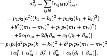
The genetic variance of the population () is the variance of the genotypic deviations,

(2)

where, for simplicity, we define the terms

and

In the absence of maternal effects (b = 0), the total variance is equivalent to that under imprinting alone (Spencer 2002).

Note that when k₁ = k₂ = k and m₁ = m₂ = m, so that imprinting is absent, Equations 1 and 2 reduce to

(3)

and

(4)

where and . These are equivalent to the values of Kempthorne (1957), using our notation (see Table 5 for the mating table showing all possible offspring genotypes for maternal effects in the absence of imprinting and Table 6 for genotypic values, breeding values, and dominance deviations under maternal effects alone).

TABLE 5.

Mating table of all possible offspring genotypes under maternal effects only

Mother (AkAl)	Father	Offspring (AiAj)	Offspring genotypic value (Gijkl)	Proportion of offspring	Frequency of mating

TABLE 6.

Genotypic values, frequencies, breeding values, and dominance deviations for additive maternal effects and no imprinting model

Genotype
Genotypic values
Frequency of genotypic values
Genotypic deviations
Female progeny mean
Male progeny mean
Female breeding value
Male breeding value
Female dominance deviations
Male dominance deviations

and .

The additive genetic variances for females () and males () are the respective variances of their breeding values:

(5)

and

(6)

The male additive variance is equivalent to that under imprinting alone (Spencer 2002) and is therefore unaffected by the addition of maternal effects to the model. In contrast, the female additive genetic variance is equivalent to that under imprinting alone (Spencer 2002) only when maternal effects are absent (b = 0). We may define progeny means and breeding values for maternal effects alone (i.e., in the absence of imprinting) (see Table 6) as described above and find that the additive genetic variances simplify to

(7)

and

(8)

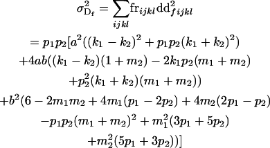
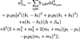
The dominance genetic variance is the variance of the dominance deviations and is not the same for females () and males ():

(9)

and

(10)

Under imprinting alone, dominance variances are equivalent for males and females (Spencer 2002). It is interesting to note that this equivalence is lost when maternal effects are included. Taking the variance of the dominance deviations for maternal effects alone (defined in Table 6), we find that

(11)

and

(12)

The nonequivalence of dominance deviation variances under imprinting and maternal effects is therefore due to differences between male and female dominance variances under maternal effects alone.

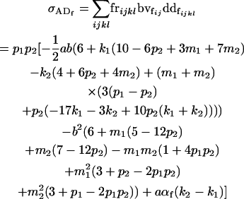
The covariances between dominance deviations and breeding values are given by

(13)

and

(14)

Under maternal effects alone these simplify to

(15)

and

(16)

and in the absence of both maternal effects and imprinting (b = 0 and k₁ = k₂), the covariances are zero and breeding values and dominance deviations are uncorrelated.

Finally, it can be easily shown that

for both maternal effects and imprinting and for maternal effects alone.

It is reassuring to note that values for the population mean, variances, and covariances under maternal effects alone are equivalent whether they are derived independently from Tables 5 and 6 or by substituting k = k₁ = k₂ and m = m₁ = m₂ into Equations 1, 2, 5, 6, 9, 10, 13, and 14.

Resemblance between relatives:

We now follow the approach of Kempthorne (1957) to calculate the mother–offspring covariance (, covariance between offspring and female parent) and father–offspring covariance (, covariance between offspring and male parent) using Table 7. Table 7 displays the genotypic values of parents and the mean value of offspring of these parents. Note that this table covers all 12 possible parent genotypes, as it is important to not average over A_kl genotypes (the male or female parent's own mother).

TABLE 7.

Genotypic values and progeny means for mother–offspring and father–offspring pairs under maternal effects and imprinting

Parent genotype	Frequency	Genotypic value	Progeny mean of females	Progeny mean of males

Then

(17)

and

(18)

Note that, following Spencer (2002), these covariances are equivalent to

(19)

and

(20)

The full-sib covariance () can be calculated with the aid of Table 8, which displays all possible genotypic values and frequencies of pairs of siblings:

(21)

TABLE 8.

Genotypic values for full-sib offspring pairs from mating combinations

Mother	Father	Offspring pair genotypic values [proportion of total offspring of mating class]	Frequency of mating class
	and
	and
	and
	and

In the absence of imprinting, setting k = k₁ = k₂ and m = m₁ = m₂, we find that

and

These covariances are equivalent to the values of Kempthorne (1957), using our notation (note that his definitions for and are not the same as ours). When imprinting is present in the absence of maternal effects (b = 0),

(also derived by Spencer 2002), and

Finally, we may also calculate the covariance between offspring who share a mother or a father. Following Spencer (2002), the covariance of half-siblings who share a mother is

(22)

and the covariance of half-sibs sharing a father is

(23)

These covariances reduce to

and

in the absence of imprinting and

and

if we assume no maternal effects (Spencer 2002).

Approach 2a:

We now follow a general least-squares approach (Lynch and Walsh 1998) to calculate population breeding values, dominance deviations, components of variance, and covariances between relatives.

We can write the genotypic value G_ijkl as the sum of the mean plus the additive () and dominance () effects,

(24)

where as above, is the average additive effect of inheriting an A_i allele from the mother, is the average additive effect of inheriting an A_j allele from the father, is the average additive effect of having a mother who received an A_k allele from her own mother, and is the average additive effect of having a mother who received an A_l allele from her own father. The dominance effects are defined below. Note that here “.” represents either an A₁ or an A₂ allele in that position.

We first calculate the average genetic values of A_iA_j genotypes using Table 3. For example, the average genotypic value of an A₁A₁ individual is

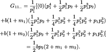Similarly,

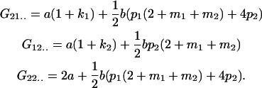It can be noted that, as expected,

The additive effect of an allele is the deviation of members of the population with the allele from the population mean. In the absence of imprinting, the parental origin of the allele has no effect. With imprinting, however, we can calculate the additive effect of the allele separately under maternal and paternal inheritance. For example, the average additive effect of an A₁ allele when inherited maternally is the average of the mean A₁A₁ and A₁A₂ genotypic values minus the population mean,

while the additive effect of an A₁ allele when inherited paternally is

The other two additive effects are thus

The dominance effects are defined as

for example,

The other dominance effects are shown below:

It is interesting to note that the dominance effects are the same for individuals with an genotype (regardless of mother) as they are for individuals with an genotype.

With the help of Table 3, we may now define average genetic values of individuals with an A_kA_l mother. For example, the average genotypic value of an individual with an A₁A₁ mother is

Similarly,

and again, as expected,

The additive effects of maternal allele may now be calculated. For example, the average additive effect of a mother with a maternally inherited A₁ allele is

while the additive effect of a mother with a paternally inherited A₁ allele is

The other two additive maternal effects are similarly

The maternal dominance effects are defined as

for example,

The other maternal dominance effects are similarly

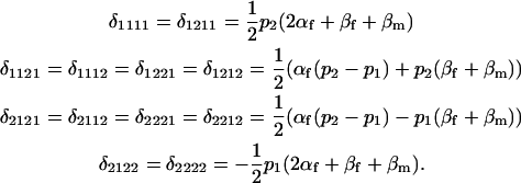
Finally, we calculate the combined offspring–mother genotype dominance deviations as

The combined dominance effects are shown below:

In approach 1, we followed the definition that the breeding value of an individual is twice the difference between the mean genotypic value of the class's offspring and the population mean (Falconer and Mackay 1996). When breeding values are equivalent for males and females, the breeding value of a genotypic class is also the sum of the additive effects of its genes (Lynch and Walsh 1998):

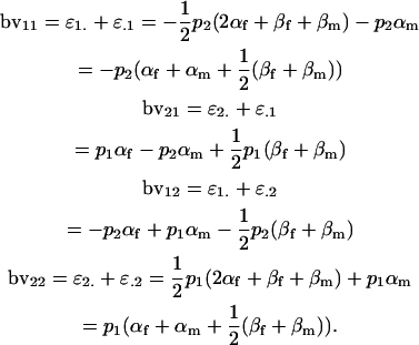For a locus influenced by imprinting and maternal effects, however, breeding values are different for males and females. Taking the mean of female and male breeding values from approach 1 (Table 4), we can see that

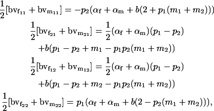which are not equivalent to the combined female and male breeding values calculated above from the sum of additive effects.

Genetic variance components:

We may now calculate variances associated with the population. The offspring genotype additive genetic variation is the variance associated with the average additive effects of alleles and can be shown to be

while the offspring genotype dominance genetic variance is the genetic variance associated with dominance effects:

Similarly we calculate the variance in the maternal genotype additive effects as

and dominance variance for maternal genotype as

The variance in combined dominance effects is

Recalling that we defined our genotypic effects as

we may write

and the total variance (var) in the population can be expressed as

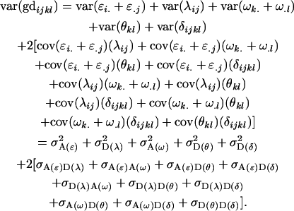(25)

The covariances (cov) of additive-by-additive and additive-by-dominance effects are

Note that all other covariances are zero. As expected, the total variance in the population (2) may be recovered from Equation 25.

Approach 2b:

Approach 2a calculated total additive and dominance effects and did not allow separate calculation of female and male additive and dominance variances as were possible in approach 1. Therefore let us redefine the additive allele effects as female and male effects, so that

where the extra subscripts on indicate female (f) and male (m) effects. These definitions allow inclusion of a parental influence on the next generation into the model. For example, a G_ijkl mother will contribute and alleles to her offspring, plus a maternal component of from her own genotype (plus dominance terms). In contrast, G_ijkl fathers will contribute only and alleles to offspring (plus a dominance term) and will not contribute a maternal term. In using these definitions we endeavor to partition the additive and dominance terms into those specific to male and female inheritance.

Following this model, terms are defined as in approach 2a. We define female offspring dominance effects as

For example,

The other female offspring dominance effects are thus

Note that dominance effects are no longer equivalent for and individuals. The mean female dominance deviation is zero.

We now calculate the combined offspring–mother genotype dominance deviations for females as

The female combined dominance deviations are therefore

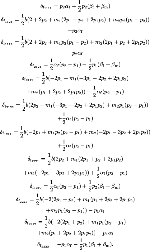The male offspring combined dominance deviations are calculated as

and are thus

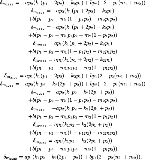Again defining the breeding value of a genotypic class as the sum of the additive effects of its genes (Lynch and Walsh 1998), we may utilize the separate male and female additive effects to calculate male and female breeding values. Hence

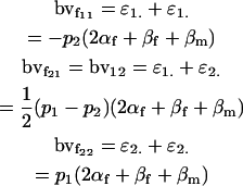for females and

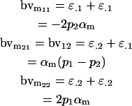for males. It is interesting to note that this approach recovers the male but not the female breeding values derived in approach 1 (Table 4).

Genetic variance components:

We may now calculate male and female variances associated with the population. The female offspring genotype additive genetic variation is the variance associated with the average additive effects of alleles inherited maternally and can be shown to be

Similarly the offspring female genotype dominance genetic variance is the genetic variance associated with the female dominance effects,

and the combined female dominance genetic variance is the variance of the combined female dominance effects,

The variances in maternal genotype additive and dominance effects are those found in approach 2a.

The female covariances are

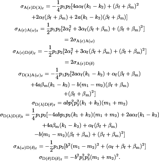The two remaining covariances are zero. As expected, the total variance in the population (2) may be recovered from Equation 25 for the corresponding female variances and covariances.

The male offspring genotype additive genetic variation is

Note that .

The male combined dominance variance is

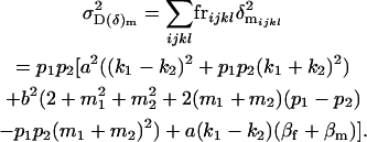Finally, the covariance between male additive and dominance effects is

Here the total variance in the population (2) is

and is equivalent to that found in Equation 2.

It is interesting to note that the male additive and dominance variances and additive-by-dominance covariance are identical to (6), (10), and (14), the variances and covariance found using a different method in approach 1. In contrast, the female variances and covariances are not immediately comparable to those found in approach 1. Further, these values cannot be recovered by ignoring maternal additive and dominance allelic effects so that we reduce the model to

and

Resemblance between relatives:

Using the separate male and female variance and covariance terms defined above and Equations 19, 20, 22, and 23 from Spencer (2002), we may calculate parent–offspring covariances and covariances between half-sibs. We start with males and find that indeed

and

In contrast, the female parent–offspring covariance (Equations 17 and 19) and covariance of half-sibs sharing a mother (Equation 22) cannot be recovered from any linear combination of our values for female variances and covariances derived using our novel approach above.

DISCUSSION

The importance of parental effects on the phenotype has long been realized. Nevertheless, the way in which various forms of parental effects alter the terms in quantitative genetic models has not always been clear. Here we show that two different kinds of parental effects—genomic imprinting and maternal genetic effects—alter the variance components in the simplest one-locus two-allele model in fundamental and revealing ways. Moreover, we find that different approaches to calculating these components, which work well for the standard model without such parental effects, cannot be relied upon when parental effects are present.

We used two approaches (Falconer and Mackay 1996; Lynch and Walsh 1998) to calculate additive, dominance, and total genetic variance. Although both methods give identical total genetic variance terms, there are differences in the partitioning of the variance into additive, dominance, and covariance terms. These methods differ in that the first approach uses progeny means to calculate breeding values, while the second method uses a least-squares approach to define breeding values as the sum of the average allelic effects. Under a standard, one-locus diallelic model (that is, without any form of parental effects), the two approaches retrieve equivalent additive and dominance effects and no correlation between additive and dominance effects. However, maternal and imprinting effects introduce both sex-dependent and generation-dependent effects that result in differences in the way additive and dominance effects are defined for the two approaches. Specifically, Falconer and Mackay (1996) (approach 1) use the variance of the breeding values to calculate additive genetic variances. Breeding values are calculated from the progeny means of each genotype, and this approach introduces a “generation” effect into the additive dominance. In contrast, Lynch and Walsh (1998) (approach 2) use additive effects of alleles to calculate additive variance. These additive allelic effects are found by averaging over the genotypic values of individuals expressing these alleles and so do not include the same generational effect as calculating breeding values does.

Approach 2 is a more straightforward method for calculating additive and dominance variances because it does not require consideration of mating tables. However, we saw above that we were not able to recover the approach 1 values for female additive and dominance variances and the additive-by-dominance covariance when we refined the least-squares approach to include male and female effects (approach 2a). It is interesting to note that approach 2a was able to recover the male variances and covariance. Clearly calculation of male breeding values (approach 1) and male allelic effects (approach 2a) by averaging over female mates and mothers, respectively, has the same overall effect.

We may examine the covariances between relatives derived in approach 1 and can see that both imprinting and maternal effects add extra terms. Ignoring imprinting and maternal effects may over- or underestimate true covariances. For example, Tables 9 and 10 calculate parent–offspring, full-sib, and half-sib covariances for six models: (i) a full model incorporating paternal inactivation and maternal effects, (ii) a model including paternal inactivation only, (iii) a full model incorporating maternal inactivation and maternal effects, (iv) a model including maternal inactivation only, (v) a model including maternal effects only, and (vi) a standard two-allele model without imprinting or maternal effects. Assuming that both maternal effects and imprinting are influencing this trait, we have calculated the true expected population covariances under both paternal inactivation (model i) and maternal inactivation (model iii). Table 9 calculates these covariances for a = 0.5 and b = 0.1 (offspring genotype has largest influence on genotypic values) while Table 10 calculates these covariances for a = 0.3 and b = 0.3 (offspring and maternal genotypes have equal influence on genotypic values). Note that because we are assuming no imprinting in models v and vi, covariances for these models need not be calculated separately for maternal and paternal inactivation as do models i–iv.

TABLE 9.

Comparison of covariance predictions using incompletely specified models of imprinting only, maternal effects only, and no imprinting or maternal effects, for a = 0.5 and b = 0.1

	Paternal inactivation		Maternal inactivation
Covariances for true full model with maternal effects (i):	Covariances for imprinting only (ii):	Covariances for true full model with maternal effects (iii):	Covariances for imprinting only (iv):	Covariances for maternal effects only (v):	Covariances for standard model (vi):
Model parameters:	,,,	,,,,	,,,	,,,,	,,	,,,
	0.1749	0.1665	0.0538	0.0135	0.0963	0.0900
	0.0103	0.0135	0.1272	0.1665	0.0688	0.0900
	0.1626	0.1551	0.1201	0.1551	0.0925	0.0901
	0.1618	0.1540	0.0131	0.0010	0.0613	0.0450
	0.0007	0.0010	0.1070	0.1540	0.0313	0.0450

TABLE 10.

Comparison of covariance predictions using incompletely specified models of imprinting only, maternal effects only, and no imprinting or maternal effects, for a = 0.3 and b = 0.3

	Paternal inactivation		Maternal inactivation
Covariances for true full model with maternal effects (i):	Covariances for imprinting only (ii):	Covariances for true full model with maternal effects (iii):	Covariances for imprinting only (iv):	Covariances for maternal effects only (v):	Covariances for standard model (vi):
Model parameters:	,,,	,,,,	,,,	,,,,	,,	,,,
	0.1816	0.1665	0.0860	0.0135	0.1013	0.0900
	0.0051	0.0135	0.0624	0.1665	0.0338	0.0900
	0.1996	0.1551	0.1231	0.1551	0.1126	0.0901
	0.1993	0.1540	0.0846	0.0010	0.1013	0.0450
	0.0003	0.0010	0.0385	0.1540	0.0113	0.0450

A number of conclusions are apparent from examination of Tables 9 and 10. For paternal inactivation and maternal effects in Table 9 (model i) we can see that . Note also that models ii, v, and vi underestimate the true values for while overestimating values for . Model ii retains the relative ordering of covariances while model v incorrectly ranks ahead of . Estimates for model vi do not compare well to the true values calculated in model i.

For maternal inactivation with maternal effects in Table 9 (model iii) the relative ordering of covariances is . Model iv overestimates while models v and vi underestimate . All three models iv, v, and vi underestimate . Model iv retains the relative ranking of covariances from the true model iii, although estimates from and order ranking of models v and vi do not compare well to model iii.

Quite different observations are apparent when examining Table 10, for covariances calculated assuming maternal effects and own genotype effects have equal impact on genotypic values of offspring. For paternal inactivation and maternal effects (model i), the relative ordering of covariances is now . Once again models ii, v, and vi underestimate while overestimating . In contrast to Table 9, however, model v now appears to best estimate relative sizes and ordering of covariances.

For maternal inactivation in Table 10, an even more surprising result is apparent. Because maternal alleles are almost completely inactivated, we would expect to rank highly, as they did in Table 9. However our covariances between relatives now follow . There is no consistent pattern of over- or underestimation of covariances when comparing to the alternative models iv, v, and vi. As was the case for paternal inactivation discussed above, model v (maternal effects alone) appears to best mimic the covariance structure. Despite maternal effects and offspring own genotype having equally weighted contributions to offspring genotypic value (a = b = 0.3), it is apparent from this example that maternal genotype effects, and not imprinting effects, have greatest impact on the covariances between relatives. Further, simulation results (data not shown) suggest that maternal effects can outweigh imprinting effects even when , especially when the difference between reciprocal heterozygotes is not large. For example, if (higher paternal than maternal expression of alleles, plus maternal effects), then .

We are likely to have population estimates for covariances between relatives. It is pertinent to assess whether we can estimate values for a, b, k₁, k₂, m₁, and m₂ given these covariances. Let us take the parameters and calculated covariances from model i in Table 9 (paternal inactivation with maternal effects). We assume , , and that heterozygotes are restrained to fall within the range of the homozygotes (that is, ). We also set , so that mother and offspring genotypes act in the same way on overall offspring genotypic value. For example, an A₂A₁ offspring with an A₂A₁ mother will have a contribution to overall offspring genotypic value of a(1 + k₁) from its own genotype and a contribution of b(1 + k₁) from its mother's genotype.

We endeavor to retrieve known parameter values for a, b, k₁ (= m₁) and k₂ (= m₂) by setting the calculated values for covariances between relatives equal to their mathematical expressions and solving simultaneously. We have five equations and four unknowns, but because all five covariances involve quadratic terms in the parameters we are trying to estimate (a, b, k₁, and k₂) they do not have unique solutions for the given calculated covariances. However, applying our range constraints gives two solutions,

(our original values) and

(Table 11, full model, row 2). Values of a and b are the same for the two solutions, maintaining the relative contribution of maternal effects to the range of genotypic values. However, it is interesting to note that the two solutions exchange values for k₁ and k₂ (and m₁ and m₂) as a consequence of our assumption of equal allele frequencies in the population. As seen in Table 9, if there are large differences between predicted values for reciprocal heterozygotes and between estimates for a and b, a much larger population value for compared to is indicative of paternal inactivation. Therefore we are able to conclude that the first solution is the true solution for the population. However, as was clear from Table 10, without large differences between a and b and k₁ and k₂, it may not be possible to determine which set of values for a, b, k₁, and k₂ is true for the population. This highlights an important theoretical restriction: it may not be possible to differentiate maternal effects from imprinting using observed population covariances—even when assumptions are made about population allele frequencies and values and ranges for k₁, k₂, m₁, and m₂.

TABLE 11.

Parameter predictions when expressions for covariances are solved for true covariance values

Model	Set of simultaneous equations solved	Constraints placed on parameters	No. of solutions to equations [no. of consistent solutions to equations]	Solutions/consistent values for parameters contained in inconsistent solutions
Full model	,,		4 [2]
Imprinting only (set b = 0 for all covariances)	,,	,	0 [0]
	,		4 [0]
	,		4 [0]
	,		4 [0]
	,		8 [2]
Maternal effects only (set k1 = k2 = k and m1 = m2 = m for all covariances)	,,	,	0 [0]
	,		16 [0]
	,		4 [0]
	,		16 [0]
	,		8 [2]
No imprinting or maternal effects (set b = 0 and k1 = k2 = k for all covariances); note now , , and further	,,	, ,	0 [0]
	,		4 [0]
	,		4 [2]

We may also assess how incorrectly specifying the model affects our estimates for a, b, k₁, k₂, m₁, and m₂. We again take the known values for covariances from model i in Table 9 and use our expressions for covariances between relatives as derived in approach 1 under the three reduced models: no imprinting (maternal effects only), no maternal effects (imprinting only), and no maternal effects or imprinting. By setting the reduced expressions for covariances equal to the true values and solving, we find that in many cases we are unable to recover consistent solutions for the reduced models (Table 11). We define consistent solutions as solutions satisfying our constraints on . The lack of consistent solutions for the reduced models is an indication that the models are incomplete and that additional genetic factors are acting that have not been specified.

Examining columns 1 and 3 in Table 11, we can see that the assumptions of the three reduced models affect the restraints that are placed on our parameters: for example, under a reduced model of maternal effects only, k₁ = k₂ = k and m₁ = m₂ = m for all covariances, and we now have a condition that . Note that this also affects the number of parameters we are solving for in each of the reduced models, and hence to find a solution we must solve for subsets of covariances, rather than using all five true covariance values (Table 11, column 2). Interestingly, a consistent solution pair was found for all three reduced models using a subset of full-sib and half-sib covariances: for imprinting only,

for maternal effects only,

and for no maternal effects or imprinting,

As we also saw in the two solutions to the full model, for the imprinting-only model k₁ (and k₂) reversed sign between two solution sets, effectively reversing the prediction from maternal to paternal inactivation of alleles. A similar result was seen in the no imprinting, no maternal effects model where the A₁ allele changed from recessive to dominant in two solutions to the same simultaneous equations. In addition, it is interesting to note that the maternal-effects model estimated a much larger maternal effect (b) than the true value, while the other two models overestimated own genotype effect (a). This in general was also true of consistent estimates for a and b contained within inconsistent solution sets for these three reduced models. As would be expected, therefore, not including maternal effects in the model will overestimate the contribution from an offspring's own genotype to genotypic values and covariances.

Many of the inconsistent solutions included imaginary numbers. Examining column 5 of Table 11, we see a large range in estimates for parameters contained within these inconsistent solutions. Perhaps not surprisingly, this result suggests that consistent parameter values contained within inconsistent solution sets should not be used to infer population parameters. It can be noted from this example that inconsistent solutions, solutions containing imaginary numbers, and even the presence of more than one solution should highlight to the researcher that an incorrect model has been employed.

From Tables 9–11 we have seen that misspecification of the model can have huge implications on parameter and covariance estimation, and it is clearly important to allow for imprinting and maternal effects when estimating parameters and covariances. Nevertheless, researchers should be aware that even in using a complete model and known covariances between a range of relatives, they may not be able to differentiate between maternal and paternal expression if maternal genotype is having a significant effect and differences between reciprocal heterozygotes are small.

References

- Bartolomei, M. S., and S. M. Tilghman, 1997. Genomic imprinting in mammals. Annu. Rev. Genet. 31: 493–525. [DOI] [PubMed] [Google Scholar]
- DeChiara, T. M., E. J. Robertson and A. Efstratiadis, 1991. Parental imprinting of the mouse insulin-like growth factor II gene. Cell 64: 849–859. [DOI] [PubMed] [Google Scholar]
- Falconer, D. S., and T. F. C. Mackay, 1996. Introduction to Quantitative Genetics, Ed. 4. Longman, Harlow, Essex, UK.
- Huck, U. W., J. B. Labov and R. D. Lisk, 1987. Food-restricting first generation juvenile female hamsters (Mesocricetus auratus) affects sex ratio and growth of third generation offspring. Biol. Reprod. 37: 612–617. [DOI] [PubMed] [Google Scholar]
- Kempthorne, O., 1957. An Introduction to Genetic Statistics. John Wiley & Sons, New York.
- Lynch, M., and B. Walsh, 1998. Genetics and Analysis of Quantitative Traits. Sinauer Associates, Sunderland, MA.
- Moore, A. J., J. B. Wolf and E. D. Brodie, III, 1998. The influence of direct and indirect genetic effects on the evolution of behavior: social and sexual selection meet maternal effects, pp. 22–41 in Maternal Effects as Adaptations, edited by T. A. Mousseau and C. W. Fox. Oxford University Press, New York.
- Morison, I. M., J. P. Ramsay and H. G. Spencer, 2005. A census of mammalian imprinting. Trends Genet. 21: 457–465. [DOI] [PubMed] [Google Scholar]
- Naumova, A. K., and S. Croteau, 2004. Mechanisms of epigenetic variation: polymorphic imprinting. Curr. Genomics 5: 417–429. [Google Scholar]
- O'Neill, M. J., R. S. Ingram, P. B. Vrana and S. M. Tilghman, 2000. Allelic expression of IGF2 in marsupials and birds. Dev. Genes Evol. 210: 18–20. [DOI] [PubMed] [Google Scholar]
- Sandovici, I., M. Leppert, P. R. Hawk, A. Suarez, Y. Linares et al., 2003. Familial aggregation of abnormal methylation of parental alleles at the IGF2/H19 and IGF2R differentially methylated regions. Hum. Mol. Genet. 12: 1569–1578. [DOI] [PubMed] [Google Scholar]
- Sandovici, I., S. Kassovska-Bratinova, J. C. Loredo-Osti, M. Leppert, A. Suarez et al., 2005. Interindividual variability and parent of origin DNA methylation differences at specific human Alu elements. Hum. Mol. Genet. 14: 2135–2143. [DOI] [PubMed] [Google Scholar]
- Shaw, R. G., and D. L. Byers, 1998. Genetics of maternal and paternal effects, pp. 97–111 in Maternal Effects as Adaptations, edited by T. A. Mousseau and C. W. Fox. Oxford University Press, New York.
- Spencer, H. G., 2002. The correlation between relatives on the supposition of genomic imprinting. Genetics 161: 411–417. [DOI] [PMC free article] [PubMed] [Google Scholar]
- Wade, M. J., 1998. The evolutionary genetics of maternal effects, pp. 5–21 in Maternal Effects as Adaptations, edited by T. A. Mousseau and C. W. Fox. Oxford University Press, New York.
- Wolf, J. B., T. T. Vaughn, L. S. Pletscher and J. M. Cheverud, 2002. Contribution of maternal effect QTL to genetic architecture of early growth in mice. Heredity 89: 300–310. [DOI] [PubMed] [Google Scholar]