Modeling Extent and Distribution of Zygotic Disequilibrium: Implications for a Multigenerational Canine Pedigree

Abstract

Unlike gametic linkage disequilibrium defined for a random-mating population, zygotic disequilibrium describes the nonrandom association between different loci in a nonequilibrium population that deviates from Hardy–Weinberg equilibrium. Zygotic disequilibrium specifies five different types of disequilibria simultaneously that are (1) Hardy–Weinberg disequilibria at each locus, (2) gametic disequilibrium (including two alleles in the same gamete, each from a different locus), (3) nongametic disequilibrium (including two alleles in different gametes, each from a different locus), (4) trigenic disequilibrium (including a zygote at one locus and an allele at the other), and (5) quadrigenic disequilibrium (including two zygotes each from a different locus). However, because of the uncertainty on the phase of the double heterozygote, gametic and nongametic disequilibria need to be combined into a composite digenic disequilibrium and further define a composite quadrigenic disequilibrium together with the quadrigenic disequilibrium. To investigate the extent and distribution of zygotic disequilibrium across the canine genome, a total of 148 dogs were genotyped at 247 microsatellite markers located on 39 pairs of chromosomes for an outbred multigenerational pedigree, initiated with a limited number of unrelated founders. A major portion of zygotic disequilibrium was contributed by the composite digenic and quadrigenic disequilibrium whose values and numbers of significant marker pairs are both greater than those of trigenic disequilibrium. All types of disequilibrium are extensive in the canine genome, although their values tend to decrease with extended map distances, but with a greater slope for trigenic disequilibrium than for the other types of disequilibrium. Considerable variation in the pattern of disequilibrium reduction was observed among different chromosomes. The results from this study provide scientific guidance about the determination of the number of markers used for whole-genome association studies.

THE extent and distribution of nonrandom associations between genes at different loci, i.e., linkage disequilibria, throughout the genome have been used often as a criterion to infer demographic and genetic events of a population in the past, such as population history and evolutionary forces governing the loci. Because of its relation with the recombination fraction, the extent of association has provided a foundation for fine-scale mapping of quantitative trait loci (QTL) that control complex diseases in humans (Ardlie et al. 2002) or economical and adaptive traits in livestock (Farnir et al. 2000; McRae et al. 2002) and plants (Remington et al. 2001). Emerging as an important model system for human health research, canines have recently received a resurgence of interest in unraveling the mysteries of mammalian genomes using linkage disequilibrium (LD) analysis (Hyun et al. 2003; Lou et al. 2003; Sutter and Ostrander 2004; Sutter et al. 2004; Lindblad-Toh et al. 2005). In a study of canine mapping, aimed to detect QTL affecting canine hip dysplasia in a multihierarchic outbred pedigree, we analyzed the extent of pairwise linkage disequilibrium to change over genetic distances with a set of microsatellite markers (240) genotyped from the entire canine genome (Lou et al. 2003).

As a common case for many comparable studies, the measure of the extent of linkage disequilibrium between different loci in our canine genetic study was based on multilocus disequilibrium at the gametic level (Weir 1996). Although such a gametic disequilibrium analysis is mathematically simple, it relies upon a fundamental assumption that the population under study is at Hardy–Weinberg equilibrium (HWE), in which individuals are assumed to be randomly mating to produce the next generations. In such an HWE population, the nonrandom associations of alleles at different loci occur only within gametes rather than between gametes. The randomly mating assumption may be violated in the canine pedigree used for our earlier study because different offspring are related to each other to a varying degree although multiple dog founders were used.

For a nonequilibrium population at Hardy–Weinberg disequilibrium (HWD), zygotic disequilibria that have power to characterize nonrandom associations at both gametic and zygotic levels (Weir 1996) may be more relevant. Earlier studies have documented possible genetic and evolutionary causes for zygotic associations in a nonequilibrium population (Haldane 1949; Bennett and Binet 1956; Charlesworth 1991; Barton and Gale 1993). In this article, we revisit our outbred canine pedigree by estimating the extent of zygotic disequilibria throughout the canine genome. Although zygotic disequilibria have been theoretically developed in the literature (see Weir 1996 for an excellent description), there is no application yet, to our best knowledge, for these measures to extensively study the structure of the genome in a case study. Recently, Yang (2000, 2002) proposed a multilocus zygotic measure for association study in a nonequilibrium population. Yang's two articles present the most thoughtful survey on zygotic disequilibrium analysis. The incorporation of zygotic disequilibrium analysis into genomic research is a necessary first step toward the formulation of an optimal strategy for characterizing genome structure and organization.

ESTIMATION OF ZYGOTIC DISEQUILIBRIUM

Genotype, allele, gamete, and nongamete frequencies:

Suppose that there is a natural or experimental population in which there are two codominant markers A with two alleles A and a and B with two alleles B and b, respectively. Let p_A and p_a (p_A + p_a = 1) as well as p_B and p_b (p_B + p_b = 1) be the corresponding allele frequencies. At each of the two loci, four different formations of zygotic genotypes lead to three distinguishable genotypes, i.e., AA, Aa, and aa for marker A and BB, Bb, and bb for marker B. The two markers form 10 genotypic configurations, but only 9 can be genetically distinguished from each other. This is because genotypic configurations and have the same genotype AaBb. Let P, subscripted and superscripted by the genotype notation, be the genotypic configuration frequencies that are individually tabulated in Table 1. It is not difficult to estimate one-marker genotype frequencies from two-marker genotypic configuration frequencies by

(1)

for marker A and

(2)

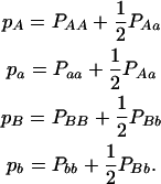
for marker B and estimate the allele frequencies from the one-marker genotype frequencies by

(3)

The two markers form four gametes, AB, Ab, aB, and ab, whose frequencies can be estimated from genotypic configuration frequencies by

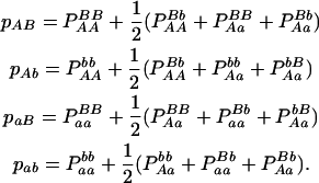(4)

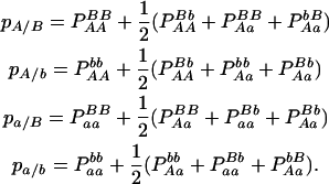
Similarly, the frequencies of nonalleles from different gametes can be estimated by

(5)

The frequencies of triple alleles from different markers are estimated as

(6)

TABLE 1.

Frequencies and observations of marker genotypes

	Marker B
Marker A	BB (2)	Bb (1)	bb (0)	Total
AA (2)				PAA = pA2 + DA
n22	n21	n20	n2·
Aa (1)				PAa = 2pApa − 2DA
n12	n11	n10	n1·
aa (0)				Paa = pa2 + DA
n02	n01	n00	n0·
Total	PBB = pB2 + DB	PBb = 2pBpb − 2DB	Pbb = pb2 + DB	1
	n·2	n·1	n·0	n

Genotype AaBb contains two different configurations or diplotypes [AB][ab] and [Ab][aB].

Complete disequilibrium parameters:

The zygotic disequilibrium is defined as the deviation of two-locus genotype frequencies from products of single-locus genotype frequencies and, thus, is composed of all nonallelic genic disequilibria at the two loci (Weir 1996). Assume that the population considered above is at HWD. This population thus has no desirable property of an equilibrium population, such as independence of different allele frequencies at the same locus (Lynch and Walsh 1998). The HWD attempts to test for two alleles at the same locus, but on different gametes, whereas (gametic) linkage disequilibrium describes two alleles on the same gametes, but at different loci. For the zygotic disequilibrium, however, there is a third test, i.e., two alleles on different gametes and at different loci.

Since the population is not in HWE, two alleles at each marker are not independent, with the coefficients of Hardy–Weinberg disequilibrium defined as

(7)

for marker A and

(8)

for marker B, respectively. The coefficient of digenic gametic linkage disequilibrium between the two markers is defined as

(9)

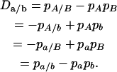
For the nonequilibrium population, digenic linkage disequilibrium that occurs between nonalleles at different gametes is defined as

(10)

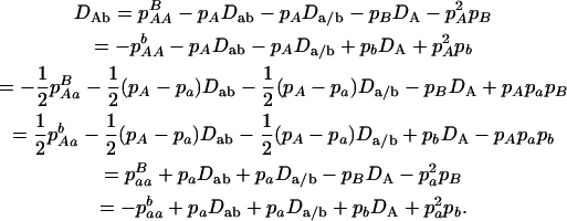
The trigenic disequilibrium between two alleles from marker A and one allele from marker B is defined as

(11)

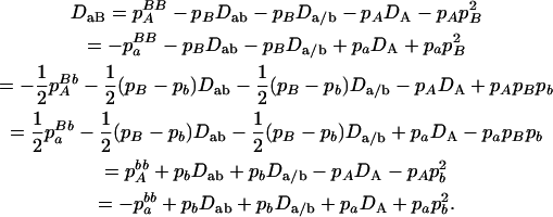
The trigenic disequilibrium between two alleles from marker A and one allele from marker B is defined as

(12)

With genotypic configuration frequencies, allele frequencies, HWD, gametic and nongametic disequilibria, and trigenic disequilibria, we can estimate the quadrigenic disequilibrium (D_AB) between two alleles from marker A and two alleles from marker B using the formulas given in Table 2 (see Weir 1996). Note that we use lower- and uppercase letters to denote gametic and zygotic disequilibria, respectively. From Table 2, we can see that each of the genotypic configuration frequencies can be expressed in terms of the allele frequencies (p_A, p_a and p_B, p_b), HWD coefficients (D_A and D_B), and gametic (D_ab) and nongametic disequilibria of different orders (D_a/b, D_Ab, D_aB, and D_AB).

TABLE 2.

Expressions of quadrigenic disequilibrium D_AB in terms of genotypic configuration frequencies, allele frequencies, and lower-order disequilibrium coefficients

Frequency	1		DA	DB	Dab	Da/b	DAb	DaB
		−1			−2pApB	−2pApB	−2pB	−2pA
		−1	pBpb		−pApB + pApb	−pApB + pApb	−pB + pb	−2pA
		−1			2pApb	−2pApb	−2pb	−2pA
		−1		pApa	−pApB + papB	−pApB + papB	−2pB	−pA + pa
	−pApapBpb	−1	pBpb	pApa	−pApB − papb	pApb + papB	−pB + pb	−pA + pa
	−pApapBpb	−1	pBpb	pApa	pApb + papB	−pApB − papb	−pB + pb	−pA + pa
		−1		pApa	pApb − papb	pApb − papb	2pb	−pA + pa
		−1			2papB	2papB	−2pB	2pa
		−1	pBpb		papB − papb	papB − papb	−pB + pb	2pa
		−1			−2papb	−2papb	2pb	2pa

Composite zygotic disequilibria:

It can be seen that 10 genotypic configurations have nine independent frequencies that are defined by two allele frequencies for each marker and seven disequilibrium parameters as defined above. But since two configurations of the double heterozygote cannot be separated in practice, it is not possible to estimate all these frequencies and disequilibrium parameters. To solve this problem, Weir (1996) suggested a set of composite disequilibrium coefficients. These include the digenic disequilibrium measured by the sum of the gametic and nongametic coefficients, i.e.,

(13)

As shown by Equations 9 and 10, Δ_ab will include the summation of gamete (p_AB) and nongamete frequencies (p_A/B). On the basis of the definitions of these two frequencies (Equations 4 and 5), Δ_ab will finally need the summation of two configuration frequencies ( and ) of the double heterozygote. Thus, Δ_ab can be estimated directly on observable genotype frequencies. Weir (1996) also defined a quadrigenic disequilibrium measured by

(14)

which can be finally measured from genotype frequencies.

The two composite digenic and quadrigenic disequilibria can make it possible to estimate the parameters on the basis of observable genotype frequencies rather than unobservable configuration frequencies. Table 3 tabulates the compositions of the composite quadrigenic disequilibrium in terms of genotype and allele frequencies and the coefficients of disequilibria with lower orders (see also Weir and Cockerham 1989).

TABLE 3.

Expressions of composite quadrigenic disequilibrium Δ_AB in terms of genotypic and allele frequencies and lower-order disequilibrium coefficients

Frequency	1		DA	DB	Δab	DAb	DaB
		−1			−2pApB	−2pB	−2pA
		−1	pBpb		−pApB + pApb	−pB + pb	−2pA
		−1			2pApb	2pb	−2pA
		−1		pApa	−pApB + papB	−2pB	−pA + pa
a	−pApapBpb	−1	pBpb	pApa		−pB + pb	−pA + pa
		−1		pApa	pApb − papb	2pb	−pA + pa
		−1			2papB	−2pB	2pa
		−1	pBpb		papB − papb	−pB + pb	2pa
		−1			−2papb	2pb	2pa

^a.

Estimates and tests:

Two markers A and B are observed for a population of size n with nine genotypes listed in Table 1. Let u and v denote the marker genotypes, u = 2 for AA, 1 for Aa, and 0 for aa and v = 2 for BB, 1 for Bb, and 0 for bb. The multinomial log-likelihood of the genotype frequencies given marker observations is written as

(15)

which gives the MLEs of the genotype frequencies as

(16)

On the basis of the estimated genotype frequencies, the allele frequencies for the two markers (p_A and p_B), the HWD coefficients (D_A and D_B), the composite digenic disequilibrium (Δ_ab), two trigenic disequilibria (D_Ab and D_aB), and the composite quadrigenic disequilibrium (Δ_AB) can be estimated.

Each of these disequilibria should be tested for its significance. The hypotheses for testing HWD are formulated by

(17)

(18)

for two different markers, respectively. The hypotheses for testing each of the zygotic disequilibria between the two markers are given as

(19)

(20)

(21)

(22)

For these hypotheses (17–22), we calculate the likelihoods under H₀ and H₁, respectively, from which the log-likelihood ratio (LR) is calculated. The LR test statistic calculated follows a χ²-distribution with 1 d.f.

The likelihoods for testing HWD on the basis of hypotheses (17) and (18) can be calculated from marginal totals of one-marker genotype frequencies and observations separately for markers A and B, respectively. For these two hypotheses, allele frequencies under H₀ can be estimated with a closed form and, thus, no EM algorithm is needed for computation. However, for the tests of hypotheses (19–22), parameter estimation under H₀ needs the implementation of numerical algorithms, like the Newton–Raphson method, because the number of unknown parameters to be estimated is less than the number of genotype frequencies. It is also possible to test whether all the disequilibrium coefficients are together equal to zero. The parameters that need to be estimated under H₀: Δ_ab = D_Ab = D_aB = Δ_AB = 0, include allele frequencies and HWD coefficients that can be estimated with a closed form. The LR value for this hypothesis should asymptotically follow the χ²-distribution with 4 d.f.

Alternatively, hypotheses (17–22) for a given disequilibrium can be tested by calculating test statistics

where denotes the estimate of the disequilibrium coefficient and is the sampling variance of the estimate, calculated by formulas given in Weir (1996). This test statistic is asymptotically χ²-distributed with 1 d.f.

Bounds and normalization:

To make zygotic disequilibria comparable between different studies, the estimates of disequilibria should be normalized. Lewontin (1964) proposed a standardized approach by expressing linkage disequilibrium as a proportion of the most extreme value. Thus, the new measure from this approach will lie between 0 (for linkage equilibrium) and | ± 1| (for complete linkage disequilibrium). A similar idea was used by Weir and Cockerham (1989) to derive bounds for trigenic and quadrigenic disequilibria for zygotic nonequilibrium analysis. More recently, Zaykin (2004) and Hamilton and Cole (2004) independently proposed algebraically equivalent bounds for a composite measure of gametic linkage disequilibrium. The bound for the composite zygotic disequilibrium has not been provided thus far. In the appendix, we provide bounds and normalized measures for all six disequilibria, D_A, D_B, Δ_ab, D_Ab, D_aB, and Δ_AB, for zygotic disequilibrium analysis. These bounds for the first five disequilibria are consistent with those published in Weir and Cockerham (1989), Zaykin (2004), and Hamilton and Cole (2004).

MATERIALS

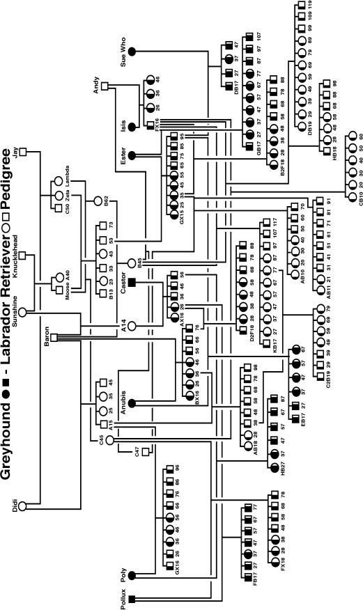
A canine pedigree was developed to map QTL responsible for canine hip dysplasia (CHD) using molecular markers. Seven founding greyhounds and six founding Labrador retrievers were intercrossed, followed by backcrossing F₁'s to the greyhounds and Labrador retrievers and intercrossing the F₁'s. A series of subsequent intercrosses among the progeny at different generation levels led to a complex network pedigree structure (Figure 1), which maximized phenotypic ranges in CHD-related quantitative traits and the chance to detect substantial linkage disequilibria (Todhunter et al. 1999, 2003a,b; Bliss et al. 2002). A total of 148 dogs from this structured pedigree were chosen for genetic analyses. This set of samples would not be appropriate for traditional gametic linkage disequilibrium analysis because the population is not randomly mating. Lou et al. (2003) estimated gametic linkage disequilibria for this pedigree on a critical foundation that the pedigree was originally derived from multiple unrelated founders. But although the resulting conclusions are consistent with the evolutionary history of dogs, Lou et al.'s analysis can be improved by estimating and testing the chromosomal distribution of zygotic disequilibria as will be done in this study.

Figure 1.—

Diagram of an outbred pedigree in dog. Squares and circles represent males and females, respectively. Solid and open portions of each symbol represent the proportion of greyhound and Labrador retriever alleles, respectively, possessed by that dog.

For the sampled dogs from the structured pedigree, 247 microsatellite markers distributed on 38 pairs of autosomes and 1 pair of sex chromosomes were genotyped to construct a linkage map for the canine genome, which displays a good coverage of each chromosome (Mellersh et al. 1997, 2000; Breen et al. 2001; Richman et al. 2001). The recombination fractions between different markers were estimated for segregating families, which are converted to genetic distances in centimorgans on the basis of a map function. The average genetic distances between two adjacent markers on each chromosome are listed in Table 4 (Breen et al. 2001).

TABLE 4.

The percentages and distributions of significant HWD and gametic and zygotic disequilibria through 39 chromosomes in the canine pedigree

Chromosome	No. markers	Averaged genetic distance (cM)	DA (%)	Δab (%)	DAb (%)	DaB (%)	ΔAB (%)
1	11	11.2	55	62	16	20	24
2	11	5.9	27	56	24	20	18
3	9	10.9	11	61	8	14	14
4	8	10.8	50	64	14	14	18
5	10	8.2	10	60	24	13	11
6	6	9.1	17	67	0	20	20
7	10	8.2	40	78	11	24	24
8	6	9.0	17	73	47	27	20
9	7	8.7	29	57	43	43	19
10	7	13.4	14	57	19	29	24
11	7	12.9	29	38	19	14	5
12	9	8.6	22	47	11	11	14
13	5	15.8	40	30	0	20	30
14	7	7.0	14	48	19	10	19
15	7	5.0	14	48	19	14	29
16	4	3.4	25	67	17	0	0
17	5	15.8	60	40	10	10	0
18	7	9.1	43	57	0	29	5
19	5	11.0	60	50	30	0	10
20	5	10.9	20	20	20	10	10
21	5	12.8	20	70	30	20	10
22	6	9.7	17	40	13	27	20
23	6	10.3	33	53	7	20	7
24	4	12.0	25	83	33	0	50
25	6	8.5	50	47	20	40	20
26	5	6.8	0	50	30	10	40
27	6	8.8	33	47	33	20	33
28	6	10.5	33	87	27	7	33
29	4	9.1	0	67	0	0	17
30	7	6.3	14	57	14	10	14
31	5	6.6	20	70	20	10	0
32	4	11.7	25	83	17	17	17
33	5	4.9	60	90	50	40	10
34	4	13.5	0	83	17	0	33
35	4	6.1	25	67	33	33	0
36	2	7.3	0	100	100	100	100
37	13	7.9	31	73	18	18	22
38	4	4.0	0	50	33	17	17
39	5	11.9	100	70	40	0	90
Overall	247	9.3	28	61	23	19	22

RESULTS

The microsatellite markers genotyped display high heterozygosity in the dog pedigree, with the number of alleles at a marker ranging from 2 to 11 (Todhunter et al. 2003b). The multialleles of the microsatellite markers are collapsed into two categories, the most frequent allele vs. all the rest pooled alleles. Thus, the simple biallelic model can be directly used to analyze the extent and distribution of zygotic disequilibria throughout the canine genome using the model developed above.

The zygotic disequilibria that describe the association between two different markers in a nonequilibrium population, like the canine pedigree as used in this study, were estimated and tested for each pair of markers located on the same chromosome. The zygotic associations were partitioned into Hardy–Weinberg disequilibria at each locus (D_A), composite gametic disequilibrium including two alleles each from a different locus (Δ_ab), trigenic disequilibria including a zygote at one locus and an allele at the other (D_Ab or D_aB), and composite quadrigenic disequilibrium including two zygotes each from a different locus (Δ_AB). All these disequilibrium coefficients were normalized using a procedure described in the appendix. All the comparisons are based on the normalized coefficients.

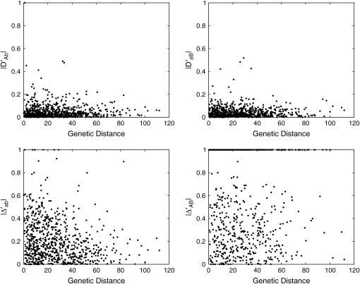
Overall, 28% of the markers genotyped were observed to deviate from HWE, but showed considerable interchromosomal variation ranging from 0 (chromosomes 26, 29, 34, 36, and 38) to 100% (sex chromosome) (Table 4). Of the four types of dilocus disequilibria, Δ_ab displays the most important impact on zygotic associations because its estimates are generally much larger than those of the other disequilibrium types. Furthermore, this disequilibrium, as well as the composite quadrigenic disequilibrium, has larger normalized values than the other types (Figure 2). Overall, the largest percentage of marker pairs is significant for Δ_ab (61%), followed by trigenic disequilibria D_Ab (23%) and D_aB (19%) and composite quadrigenic disequilibrium Δ_AB (22%). The percentages of marker pairs that exhibit significant associations vary among different chromosomes (Table 4).

Figure 2.—

Distributions of gametic and zygotic disequilibria values observed between syntenic marker pairs as a function of genetic distance in centimorgans.

Figure 2 illustrates the patterns of the relationship between zygotic disequilibria, Δ_ab, D_Ab, D_aB, and Δ_AB, and genetic distances, all exhibiting a trend of decay with increased map distance. All the types of zygotic disequilibria occur more frequently between pairs of markers separated by <40 cM than between those separated by >40 cM. As compared with D_Ab and D_aB, Δ_ab and Δ_AB tend to extend within a broader region of the canine genome. Both Δ_ab and Δ_AB decay with map distance, to a greater extent for the former than for the latter.

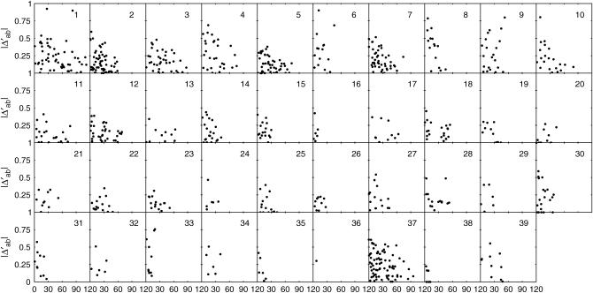
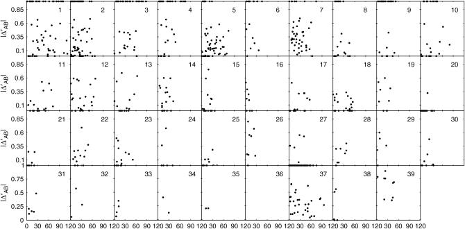
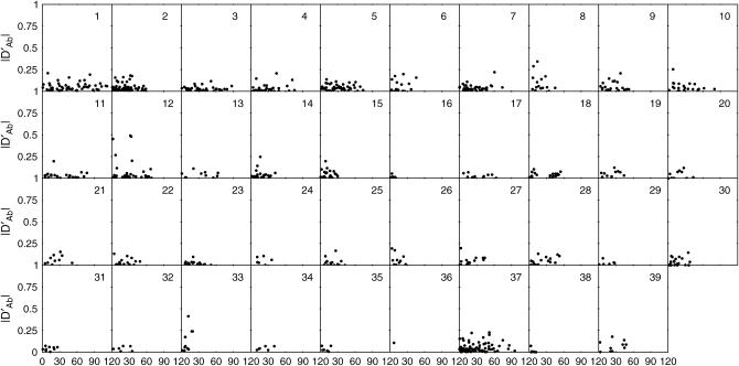
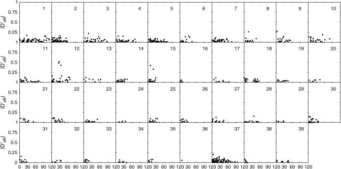
Each of the four types of zygotic association was plotted against the map distance separately for individual chromosomes (Figures 3–6). Although the data are sparse, a general trend can be observed for the extent of zygotic disequilibria; i.e., whereas the distributions of D_Ab and D_aB follow a similar pattern among different chromosomes, there is substantial interchromosomal variation in the extent and distribution of Δ_ab and Δ_AB over the canine genome.

Figure 3.—

Interchromosomal heterogeneity in the extent and distribution of digenic linkage disequilibrium Δ_ab among 39 chromosomes.

Figure 6.—

Interchromosomal heterogeneity in the extent and distribution of quadrigenic linkage disequilibrium Δ_AB among 39 chromosomes.

Figure 4.—

Interchromosomal heterogeneity in the extent and distribution of trigenic linkage disequilibrium D_Ab among 39 chromosomes.

Figure 5.—

Interchromosomal heterogeneity in the extent and distribution of digenic linkage disequilibrium D_aB among 39 chromosomes.

MONTE CARLO SIMULATION

To our best knowledge, this is the first study of the distribution of zygotic disequilibrium across the genome in a nonequilibrium population. Given the tradition that most current linkage disequilibrium analyses are based on gametic associations without a test for zygotic disequilibria, we perform a reciprocal simulation study to examine the influence of such analyses on the power of the disequilibrium test in a nonequilibrium population. According to this reciprocal simulation study, data are simulated, respectively, under zygotic and gametic disequilibrium models, but are subject to separate analyses by each of these two models.

Simulated data by the zygotic model:

Table 5 lists four simulation designs in each of which all types of associations occur for an assumed nonequilibrium population. But these four designs are different in terms of the allocation pattern of zygotic associations. In designs 1 and 2, a large composite digenic disequilibrium is contributed mainly by gametic or nongametic disequilibrium, respectively. Designs 3 and 4 purport to have a large trigenic and a quadrigenic disequilibrium, respectively. The sample size is 150, mimicking the canine example used above. The simulated data are analyzed by both the gametic and the zygotic disequilibrium models. The simulation under each design is repeated 200 times to calculate the precision of parameter estimation and statistical power of disequilibrium detection. The results from this simulation study (Table 6) are summarized as follows:

1. The zygotic disequilibrium model provides reasonable estimation of any type of disequilibria and shows a great power to detect disequilibria for a nonequilibrium population under simulation.

2. As expected, the gametic linkage disequilibrium model can estimate only gametic linkage disequilibrium, but when used to estimate a nonequilibrium population, its estimation of this parameter is largely biased. Actually, the gametic model tends to estimate the composite gametic and nongametic disequilibrium when both exist, but its estimation precision is very poor. If the composite digenic disequilibrium is mainly due to the nongametic disequilibrium (design 2), the gametic disequilibrium model cannot be used, given its large estimation error.

3. The gametic disequilibrium model can accurately estimate allele frequencies, but cannot provide precise estimation of these parameters. The second and third findings indicate that gametic disequilibrium analysis should never be used for a nonequilibrium population and that the test for zygotic disequilibrium is always crucial before gametic disequilibrium analysis is used.

TABLE 5.

Given parameter values for simulation under different designs

Design	pA	pB	DA	DB	Dab	Da/b	DAb	DaB	DAB
1	0.5	0.6	0.05	0.05	0.10	0.01	0.01	0.01	0.01
2	0.5	0.6	0.05	0.05	0.01	0.10	0.01	0.01	0.01
3	0.5	0.6	0.05	0.05	0.02	0.02	0.03	0.03	0.01
4	0.5	0.6	0.05	0.05	0.02	0.02	0.01	0.01	0.03

TABLE 6.

Maximum-likelihood estimates of parameters and the square roots of their mean square errors (in parentheses) estimated by the zygotic- and gametic-LD models for the data simulated under the zygotic-LD model of different designs

Model	pA	pB	DA	DB	Δab	DAb	DaB	ΔAB	Dab
Design 1
True	0.5	0.6	0.05	0.05	0.11	0.01	0.1	0.008
Zygotic	0.5	0.6	0.05	0.05	0.11	0.01	0.1	0.007
(0.006)	(0.006)	(0.005)	(0.005)	(0.005)	(0.005)	(0.005)	(0.005)
Gametic	0.5	0.6	—	—	—	—	—	—	0.078
(0.022)	(0.022)	—	—	—	—	—	—	(0.022)
Design 2
True	0.5	0.6	0.05	0.05	0.11	0.01	0.1	0.008
Zygotic	0.5	0.6	0.05	0.05	0.11	0.01	0.1	0.007
(0.004)	(0.004)	(0.004)	(0.004)	(0.004)	(0.003)	0.003)	(0.003)
Gametic	0.5	0.6	—	—	—	—	—	—	0.078
(0.068)	(0.067)	—	—	—	—	—	—	(0.068)
Design 3
True	0.5	0.6	0.05	0.05	0.04	0.03	0.03	0.0092
Zygotic	0.5	0.6	0.05	0.05	0.04	0.03	0.03	0.0090
(0.007)	(0.007)	(0.006)	(0.006)	(0.006)	(0.006)	(0.006)	(0.0061)
Gametic	0.5	0.6	—	—	—	—	—	—	0.041
(0.022)	(0.022)	—	—	—	—	—	—	(0.021)
Design 4
True	0.5	0.6	0.05	0.05	0.04	0.01	0.01	0.0292
Zygotic	0.5	0.6	0.05	0.05	0.04	0.01	0.01	0.0280
(0.004)	(0.004)	(0.004)	(0.004)	(0.004)	(0.003)	(0.003)	(0.0034)
Gametic	0.5	0.6	—	—	—	—	—	—	0.047
	(0.027)	(0.027)	—	—	—	—	—	—	(0.028)

Simulated data by gametic model:

As a follow-up, we simulated the data for an equilibrium population by a gametic linkage disequilibrium model. The simulated data were analyzed by both the zygotic and the gametic models (Table 7). It can be seen that the zygotic model estimates the coefficient of linkage disequilibrium as precisely as the gametic model. The result from this simulation indicates that the zygotic model is powerful to estimate the degree of linkage disequilibrium for an equilibrium population. In conjunction with the results from the simulation by the zygotic disequilibrium model, it is concluded that the zygotic model is more general than the gametic model.

TABLE 7.

Maximum-likelihood estimates of parameters and the square roots of their mean square errors (in parentheses) estimated by the zygotic- and gametic-LD models for the data simulated under the gametic-LD model

Model	pA	pB	DA	DB	Δab	DAb	DaB	ΔAB	Dab
True	0.5	0.6	0	0	0.08	0	0	0	0.08
Zygotic	0.5	0.6	0	0	0.08	0	0	0
(0.005)	(0.005)	(0.004)	(0.004)	(0.004)	(0.004)	(0.004)	(0.004)
Gametic	0.5	0.6	—	—	—	—	—	—	0.08
	(0.003)	(0.003)	—	—	—	—	—	—	(0.003)

DISCUSSION

The characterization of the architecture of linkage disequilibrium in the genome is an area of explosive recent growth (Farnir et al. 2000; Remington et al. 2001; Ardlie et al. 2002; Hyun et al. 2003; Lou et al. 2003; Sutter and Ostrander 2004; Sutter et al. 2004; Lindblad-Toh et al. 2005) because the positional cloning of genes underlying common complex diseases relies on the identification of linkage disequilibrium between genetic markers and disease. Traditional linkage disequilibrium is defined as the nonrandom association between alleles at different loci in gametes or haplotypes. The estimation of such gametic linkage disequilibrium between different loci requires the assumption that the population under consideration is randomly mating, following HWE. However, for many nonequilibrium populations that are founded by a small number of ancestors and/or are frequently under evolutionary pressure, such as mutation, genetic drift, and population admixture and structure, or under artificial selection (Lynch and Walsh 1998), HWE may be violated and, therefore, a new analysis that relaxes the random-mating assumption should be formulated. Weir (1996) introduced the concept of zygotic association or zygotic disequilibrium that can characterize the disequilibria between different loci in a nonequilibrium population. Recently, Yang (2000, 2002) proposed a multilocus statistic to examine zygotic associations in nonequilibrium populations. Different disequilibria due to a single locus or multiple loci can be summarized in such a statistic.

In a multigenerational canine pedigree constructed by several founders (Todhunter et al. 1999), individual dogs are related to each other and, thus, sampled dogs from this pedigree violate the HWE assumption due to inbreeding. For this reason, zygotic disequilibrium should be more appropriate for this related pedigree to investigate the extent and distribution of associations throughout the canine genome. We found extensive linkage disequilibria in a broad region of chromosomes (≥40 cM), as compared with the human genome, even for the most isolated human populations (Hall et al. 2002; Varilo et al. 2003; Tenesa et al. 2004). This finding seems to be comparable with those of earlier linkage disequilibrium studies of purebred dogs (Hyun et al. 2003; Sutter et al. 2004). The extent of linkage disequilibrium across the chromosomes was also investigated for the same data set by the gametic linkage disequilibrium model (Lou et al. 2003). Although the results of the two models are broadly in agreement, the linkage disequilibrium detected by the zygotic model seems to be distributed more extensively over the genome than that detected previously by the gametic model. Given the finding from the simulation, the gametic model tends to estimate a combined gametic and nongametic linkage disequilibrium, i.e., composite digenic disequilibrium, and, therefore, to provide a biased estimate of gametic linkage disequilibrium especially when a large nongametic linkage disequilibrium exists. The extensive distribution of linkage disequilibrium in the canine genome detected by the zygotic model suggests that a relatively small number of markers will be required for whole-genome association mapping in dogs. However, an optimal number of markers should be determined separately for individual chromosomes, because the extent of linkage disequilibrium shows substantial interchromosomal variation. Historically, different degrees of selection pressure may have been operational on various chromosomes, which causes interchromosomal differentiation in linkage disequilibrium extent (Sutter and Ostrander 2004; Ostrander and Wayne 2005; Parker and Ostrander 2005).

The most significant contribution of this article may lie in the first systematic use of a zygotic disequilibrium analysis to characterize the extent of disequilibrium for a nonequilibrium population of canines although the conclusions obtained from our analysis may be explained only for the specific canine pedigree used, in which individual dogs are related to different extents. On the basis of simulation analyses, the idea and concept of zygotic disequilibrium can be readily applied to any population genetic studies. Results from simulation analyses indicate that a popular gametic linkage disequilibrium analysis when employed to understand the genetic structure of the population at HWD should be used with caution because the results from this analysis will be misleading. The zygotic disequilibrium model that does not rely on the assumption of random mating has great power to detect various types of disequilibrium at different orders. Therefore, it is safe to say that the zygotic disequilibrium model covers well the gametic disequilibrium model in practical population genetic studies.

In this study, the zygotic disequilibrium model mostly modified from Weir (1996) was proposed on the basis of biallelic markers although the data from a canine genetic project are multiallelic microsatellites. Given the current modest sample size used, it should be more reasonable to collapse multiple alleles into bialleles than to direly use the multiallelic zygotic model in terms of reducing the number of parameters being estimated. Also, with the development of high-throughput technologies for single-nucleotide polymorphism (SNP) markers, the biallelic model will be useful to analyze the genetic architecture of zygotic disequilibria over the entire genome for any nonequilibrium or isolated populations including humans and other agriculturally important species. However, when a sample size is sufficiently large, the multiallelic model, in which the number of disequilibrium parameters increases exponentially with the number of alleles, will be more informative than the biallelic model based on the collapsing of alleles. Technically, it is straightforward, although tedious, to model zygotic disequilibria with multiallelic markers. For example, consider two triallelic markers that each form six distinguishable genotypes. A total of 35 genotype frequencies for these two markers contain four allele frequencies, six HWD coefficients, four composite digenic disequilibria, 12 trigenic disequilibria, and nine composite quadrigenic disequilibria. Also, our zygotic model can be readily extended to manipulate three biallelic markers at the same time as seen in Yang (2000, 2002). With these extensions and modifications, the zygotic disequilibrium analysis will provide a routine tool for the identification of the overall picture of disequilibria across the genome. The results obtained from the zygotic disequilibrium model, like those for canine genetics in this study, will have important implications for the gene mapping of complex traits.

APPENDIX

In what follows, we derived the ranges of the disequilibrium parameters for a nonequilibrium population and defined the normalized zygotic disequilibrium in a way as for gametic LD (Lewontin 1964, 1988). On the basis of Equations 7 and 8, the ranges of the HWD coefficients are expressed as

for marker A, and

for marker B.

For the composite gametic disequilibrium, the range is derived, on the basis of Equations 9, 10, and 13, as

where A = 2p_Ap_b, B = 2p_ap_b, C = p²_Ap_b + p²_ap_B + p_Ap_a, , E = 2p_Ap_B, F = 2p_ap_b, , , , and . The normalized Δ_ab is defined as

where

On the basis of Equations 11 and 12, two trigenic disequilibria have the ranges expressed, respectively, as

where A = 2p_Ap_ap_b, , , , , , , H = p_Ap_B, I = p_ap_B, , , , , , , , , , , , , , , , , , , , and

where A′ = 2p_ap_Bp_b, , , , , , , , , , , , , , , , , , , , , , , , , , , and . The normalized D_Ab and D_aB are defined, respectively, as

where

and

where

On the basis of Table 3, the range of the composite quadrigenic disequilibrium is expressed as

where , , , , , , , , and . The normalized Δ_ab is defined as

where

References

- Ardlie, K. G., L. Kruglyak and M. Seielstad, 2002. Patterns of linkage disequilibrium in the human genome. Nat. Rev. Genet. 3: 299–309. [DOI] [PubMed] [Google Scholar]
- Barton, N. H., and K. S. Gale, 1993. Genetic analysis of hybrid zones, pp. 13–45 in Hybrid Zones and the Evolutionary Process, edited by R. G. Harrison. Oxford University Press, Oxford.
- Bennett, J. H., and F. E. Binet, 1956. Association between Mendelian factors with mixed selfing and random mating. Heredity 10: 51–55. [Google Scholar]
- Bliss, S., R. J. Todhunter, R. Quaas, G. Casella, R. L. Wu et al., 2002. Quantitative genetics of traits associated with hip dysplasia in a canine pedigree constructed by mating dysplastic Labrador retrievers with unaffected greyhounds. Am. J. Vet. Res. 63: 1029–1035. [DOI] [PubMed] [Google Scholar]
- Breen, M., S. Jouquand, C. Renier, C. S. Mellersh, C. Hitte et al., 2001. Chromosome-specific single-locus FISH probes allow anchorage of an 1800-marker integrated radiation-hybrid/linkage map of the domestic dog genome to all chromosomes. Mamm. Genome 11: 1784–1795. [DOI] [PMC free article] [PubMed] [Google Scholar]
- Charlesworth, B., 1991. The evolution of sex chromosomes. Science 251: 1030–1033. [DOI] [PubMed] [Google Scholar]
- Farnir, F., W. Coppieters, J. J. Arranz, P. Berzi, N. Cambisano et al., 2000. Extensive genome-wide linkage disequilibrium in cattle. Genome Res. 10: 220–227. [DOI] [PubMed] [Google Scholar]
- Haldane, J. B. S., 1949. The association of characters as a result of inbreeding and linkage. Ann. Eugen. 15: 15–23. [DOI] [PubMed] [Google Scholar]
- Hall, D., E. M. Wijsman, J. L. Roos, J. A. Gogos and M. Karayiorgou, 2002. Extended intermarker linkage disequilibrium in the Afrikaners. Genome Res. 12: 956–961. [DOI] [PMC free article] [PubMed] [Google Scholar]
- Hamilton, D. C., and D. E. Cole, 2004. Standardizing a composite measure of linkage disequilibrium. Ann. Hum. Genet. 68: 234–239. [DOI] [PubMed] [Google Scholar]
- Hyun, C., L. J. Filippich, R. A. Lea, G. Shepherd, I. P. Hughes et al., 2003. Prospects for whole genome linkage disequilibrium mapping in domestic dog breeds. Mamm. Genome 14: 640–649. [DOI] [PubMed] [Google Scholar]
- Lewontin, R. C., 1964. The interaction of selection and linkage. I. General considerations; heterotic models. Genetics 49: 49–67. [DOI] [PMC free article] [PubMed] [Google Scholar]
- Lewontin, R. C., 1988. On measures of gametic disequilibrium. Genetics 120: 849–852. [DOI] [PMC free article] [PubMed] [Google Scholar]
- Lindblad-Toh, K., C. M. Wade, T. S. Mikkelsen, E. K. Karlsson, D. B. Jaffe et al., 2005. Genome sequence, comparative analysis and haplotype structure of the domestic dog. Nature 438: 803–819. [DOI] [PubMed] [Google Scholar]
- Lou, X.-Y., R. J. Todhunter, M. Lin, Q. Lu, T. Liu et al., 2003. The extent and distribution of linkage disequilibrium in canine. Mamm. Genome 14: 555–564. [DOI] [PubMed] [Google Scholar]
- Lynch, M., and B. Walsh, 1998. Genetics and Analysis of Quantitative Traits. Sinauer Associates, Sunderland, MA.
- McRae, A. F., J. C. McEwan, K. G. Dodds, T. Wilson, A. M. Crawford et al., 2002. Linkage disequilibrium in domestic sheep. Genetics 160: 1113–1122. [DOI] [PMC free article] [PubMed] [Google Scholar]
- Mellersh, C. S., A. A. Langston, G. M. Acland, M. A. Fleming, K. Ray et al., 1997. A linkage map of the canine genome. Genomics 46: 326–336. [DOI] [PubMed] [Google Scholar]
- Mellersh, C. S., C. Hitte, M. Richman, F. Vignaux, C. Priat et al., 2000. An integrated linkage-radiation hybrid map of the canine genome. Mamm. Genome 11: 120–130. [DOI] [PubMed] [Google Scholar]
- Parker, H. G., and E. A. Ostrander, 2005. Canine genomics and genetics: running with the pack. PLoS Genet. 1(5): e58. [DOI] [PMC free article] [PubMed] [Google Scholar]
- Ostrander, E. A., and R. K. Wayne, 2005. The canine genome. Genome Res. 15: 1706–1716. [DOI] [PubMed] [Google Scholar]
- Remington, D. L., J. M. Thornsberry, Y. Matsuokadagger, L. M. Wilson, S. R. Whitt et al., 2001. Structure of linkage disequilibrium and phenotypic associations in the maize genome. Proc. Natl. Acad. Sci. USA 98: 11479–11484. [DOI] [PMC free article] [PubMed] [Google Scholar]
- Richman, M., C. S. Mellersh, C. Andre, F. Gailbert and E. A. Ostrander, 2001. Characterization of a minimal screening set of 172 microsatellite markers for genome-wide screens of the canine genome. J. Biochem. Biophys. Methods 47: 137–149. [DOI] [PubMed] [Google Scholar]
- Sutter, N. B., and E. A. Ostrander, 2004. Dog star rising: the canine genetic system. Nat. Rev. Genet. 5: 900–910. [DOI] [PubMed] [Google Scholar]
- Sutter, N. B., M. A. Eberle, H. G. Parker, B. J. Pullar, E. F. Kirkness et al., 2004. Extensive and breed-specific linkage disequilibrium in Canis familiaris. Genome Res. 14: 2388–2396. [DOI] [PMC free article] [PubMed] [Google Scholar]
- Tenesa, A., A. F. Wright, S. A. Knott, A. D. Carothers, C. Hayward et al., 2004. Extent of linkage disequilibrium in a Sardinian sub-isolate: sampling and methodological considerations. Hum. Mol. Genet. 13: 25–33. [DOI] [PubMed] [Google Scholar]
- Todhunter, R. J., G. M. Acland, M. Olivier, A. J. Williams, M. Vernier-Singer et al., 1999. An outcrossed canine pedigree for linkage analysis of hip dysplasia. J. Hered. 90: 83–92. [DOI] [PubMed] [Google Scholar]
- Todhunter, R. J., G. Casella, S. P. Bliss, G. Lust, A. J. Williams et al., 2003. a Power of a dysplastic Labrador retriever-greyhound pedigree for linkage analysis of hip dysplasia. Am. J. Vet. Res. 64: 418–424. [DOI] [PubMed] [Google Scholar]
- Todhunter, R. J., S. R. Bliss, S. R. Quaas, G. Lust, G. Casella et al., 2003. b Genetic structure of susceptibility traits for hip dysplasia and microsatellite informativeness of an outcrossed canine pedigree. J. Hered. 94: 39–48. [DOI] [PubMed] [Google Scholar]
- Varilo, T., T. Paunio, A. Parker, M. Perola, J. Meyer et al., 2003. The interval of linkage disequilibrium (LD) detected with microsatellite and SNP markers in chromosomes of Finnish populations with different histories. Hum. Mol. Genet. 12: 51–59. [DOI] [PubMed] [Google Scholar]
- Weir, B. S., 1996. Genetic Data Analysis II. Sinauer Associates. Sunderland, MA.
- Weir, B. S., and C. C. Cockerham, 1989. Complete characterization of disequilibrium at two loci, pp. 86–110 in Mathematical Evolutionary Theory, edited by M. W. Feldman. Princeton University Press, Princeton, NJ.
- Yang, R.-C., 2000. Zygotic associations and multilocus statistics in a nonequilibrium diploid population. Genetics 155: 1449–1458. [DOI] [PMC free article] [PubMed] [Google Scholar]
- Yang, R.-C., 2002. Analysis of multilocus zygotic associations. Genetics 161: 435–445. [DOI] [PMC free article] [PubMed] [Google Scholar]
- Zaykin, D. V., 2004. Bounds and normalization of the composite linkage disequilibrium coefficient. Genet. Epidemiol. 27: 252–257. [DOI] [PubMed] [Google Scholar]