SPRAWL IN THE 1990S Measurement, Distribution, and Trends

Abstract

Although sprawl is a growing national debate, there have been few efforts to measure or monitor changes in degree of sprawl over time. By using a methodology that employs census data, this sprawl index allows computation of levels of sprawl and examination of temporal and geographic changes. The results show that sprawl has increased over the past decade in many metropolitan areas. There are important geographic variations in sprawl, implying that it is neither inevitable nor universal.

URBAN SPRAWL IN THE UNITED STATES

For many people concerned about the quality of life in the United States, the level of sprawl has become an important issue. Although rarely precisely defined or quantified, sprawl has been proposed to be a contributor to most, if not all, contemporary U.S. urban and environmental problems including inner-city abandonment, racial segregation, income inequality, destruction of open space, loss of farmland, excess energy use, overdependence on cars, high taxes, poor health, crime, destruction of community, water pollution, and air pollution (Burchell et al. 1998; Bullard, Johnson, and Torres, 2000; Jackson, 1985; Duany, Plater-Zyberk, and Speck 2000; Kunstler 1993; Popenoe 1979; Heinlich and Andersen 2001; Freeman 2001). Sprawl has been said to accompany almost every unwanted or unattractive aspect of U.S. urban life. Opponents of large discount retail establishments, new housing developments, and new transportation projects have all tagged their targets as sprawl or sprawl enabling (Beaumont 1997). Although acknowledging that the United States has higher levels of sprawl, others have found decreasing urban densities and increasing sprawl to be worldwide phenomena. (Sheehan 2001) On the other had, some authors have claimed that sprawl or its component attributes are desirable and may have important benefits (Black 1996; Ohls and Pines 1975; Gordon and Richardson 1997; Hayward 1998; Kahn 2001). Still other authors find that sprawl has both positive and negative attributes (Downs 1999; Heim 2001) or that the cost of controlling sprawl creates problems of its own (Brueckner 1990; Lehrer and Milgram 1996). Without specifically defining sprawl, other authors have attempted to assess sprawl's impact on cities and the environment (Henderson and Arindam 1996). These associations may or not be true, but until sprawl can be quantified in a useful manner, it will be difficult to understand the relationship of sprawl to these issues or to prioritize the place of anti-sprawl measures in the effort to meet these challenges.

The lack of a clear definition of sprawl and ill-defined means of measuring it have inhibited debate on the effects, significance, and potential responses to sprawl. A clear, concise definition of sprawl would give more weight to arguments about the consequences of sprawl. A useable sprawl scale would enable those concerned about sprawl to measure it, track changes over time, and monitor its impact on the environment.

A related set of issues involves how sprawl has changed over the past decade and whether there are patterns in how sprawl varies across the country. Is sprawl increasing? Are some parts of the country more affected by sprawl than others? Is sprawl always correlated with population growth? By developing a utilitarian definition and measurement of sprawl, some of the answers to these questions can be identified.

PAST EFFORTS TO DEFINE AND MEASURE SPRAWL

In the absence of a clear way to identify and measure sprawl, it tends to be defined as a series of characteristics or attributes. This means that sprawl tends to need visual confirmation and that its definition has varied in time and space as the opinions of observers have differed. Consequently, it is unclear what is meant by sprawl. In general, sprawl has been described as containing one or more of the following elements:

• low-density development

• separation of land uses

• leapfrog development

• strip retail development

• automobile-dependent development

• development at the periphery of an urban area at the expense of its core

• employment decentralization

• loss of peri-urban, rural agriculture, and open space; and

• fragmented governmental responsibility and oversight. (Johnson 2001)

It is not immediately apparent how all the aforementioned attributes can be measured. Particularly in the context of continuing growth, development, and change in urban areas and the country as a whole, these descriptions might more or less capture every metropolitan area. Internationally, except perhaps for certain walled cities at distinct periods of time, it is likely that all urban areas contain at least some of these characteristics. The challenge is to use these elements—or an aggregate of them—as the basis for a measurable sprawl index.

There have been attempts to develop measures of sprawl. Galster et al. (2000) identified eight dimensions of sprawl: density, continuity, concentration, compactness, centrality, nuclearity, diversity, and proximity. They developed measures for these dimensions, primarily using grids of one mile or less along with Geographic Information Systems (GISs) and field surveys. They tested their definition of sprawl on six of the dimensions using data on housing in 13 metropolitan areas. They then ranked the metropolitan areas on each dimension and combined the rankings, giving equal weight to each dimension, to develop an overall sprawl score.

Although an important milestone in conceptualizing the attributes of sprawl, the Galster-Hanson methodology is awkward because it relies on complex use of GIS and detailed knowledge of local conditions for its computation. It is unlikely that such a methodology could be used to analyze all metropolitan areas in the United States and even less likely to have international applications. Its best use is as an analytical framework for evaluating other measures of sprawl. Their technique may also prove valuable for case studies documenting the degree and causes of sprawl in individual metropolitan areas. Similarly, Ewing (1997) defined sprawl as a collection of indicators that included poor accessibility and lack of functional open space. Again, although good for describing individual circumstances of sprawl, these indicators are difficult to quantify on a national scale.

Several researchers have focused on density for a measure of sprawl. Fulton et al. (2001, 3) defined density as the “population of a metropolitan area divided by the amount of urbanized land in that metropolitan area.” They pointed out that U.S. Census Bureau definitions of metropolitan area size are misleading. If the basic census definition is used—agglomerations of counties that are wholly or partly contained in a metropolitan area—then large areas of included rural area skew resulting density results. For example, the Riverside-San Bernardino metropolitan area includes the sparsely inhabited Mohave Desert because San Bernardino County is one component county of the metropolitan area. Nelson used urbanized area to assess density (Nelson 1999). But the census definition of urbanized area, more or less contiguous census tracts with a population density greater than 1,000 persons per square mile along with other associated areas, results in a large area of developed land not being included in the geographic base of the analysis. In addition, Kline (2000) points out that the census definition of urbanized area is fluid and changes over time in relation to the change in population. As an alternative, Fulton et al. and Kline use surveys by the National Resources Inventory conducted by the U.S. Department of Agriculture that estimate the amount of developed land in each county. Because these surveys do not coincide with census years, these authors estimate population for the survey years by extrapolation from the decennial census. Fulton et al. report their findings as persons per urbanized area with a minimum population density of 200 persons per square mile as the threshold for inclusion in an urbanized part of a metropolitan area. Kline uses total persons per total square miles. Neither author makes any conclusion, however, as to what point density is associated with sprawl, although presumably the lower the density, the greater the amount of sprawl. The lack of coordination with census data is a serious drawback of both the Fulton et al. and Kline studies. It complicates the count of people in a metropolitan area because of potential inaccuracies of intercensus population projections.

In two 2001 studies, a gauge of job decentralization was used as a sprawl measure (Glaeser, Kahn, and Chu 2001; Glaeser and Kahn 2001). They used county business pattern data reported by the U.S. Census Bureau and organized on a zip-code level as a means to determine the number of jobs within 3 miles, between 3 and 10 miles, and between 10 and 35 miles from the central business district (CBD) of a metropolitan area. The 1982 Economic Census Geographic Manual defines the center point of each CBD. The authors used the percentage of jobs within each of these three rings to define four types of metropolitan areas: dense, centralized, decentralized, and extremely decentralized. In another study, Kahn (2001) used these data to construct a different sprawl index based on the share of employment outside the 10-mile circle from the CBD center point.

Centralization, particularly the concentration of employment within and near the CBD of a metropolitan area, is one important dimension of sprawl. The lack of strong downtown is often seen as evidence of sprawl. However, an analysis solely founded on job distribution is less indicative of sprawl than one that uses residential patterns of development because housing occupies a larger percentage of an urban land area than employment. Jobs are almost always concentrated to some degree (excluding only single-employee firms and people working at home), but housing is more easily dispersed. Many households do not have any employed persons, and some metropolitan areas have developed around retirees, lessening the importance of employment and employment centers. In addition, both studies of job decentralization and employment sprawl can be criticized because they are influenced by the size of metropolitan areas. Larger metropolitan areas will have a higher percentage of jobs outside the 3- or 10-mile ring of the CBD simply because they are larger. The census found that metropolitan areas varied in size from 56,000 to more than 8 million in 2000. Ideally, a sprawl measure should act proportionately the same on all of them. These concerns aside, the employment concentration-based sprawl index measures an important attribute of sprawl and could potentially relate to its other dimensions.

The New York Times published an analysis of sprawl patterns using the 2000 census (Firestone 2001). The author defined nonurban census tracts as those with fewer than 350 persons per square mile and urban tracts as those with a density of at least 3,200 persons per square mile. The problem with this analysis is that it did not set a point at which a metropolitan area's mix of urban and suburban densities becomes sprawl. Virtually all metropolitan areas will contain some tracts that have low population densities because some tracts will be primarily parkland, industrial, or otherwise nonresidential in nature. For example, census tracts that contain airports or large industrial facilities could have few people and low population densities. Other tracts might straddle an urban growth boundary so that half the tract is densely developed and the other portion is not inhabited.

In separate studies, Mieszkowski and Mills (1993) and Jordan, Ross, and Usowski (1998) use density gradients to determine the degree to which population is located at a distance from the centers of cities. This combination of density and distance from the center point of a metropolitan area indicates how far the population has moved toward the periphery. The greater the degree to which a population has decentralized, the lower the density gradient. Jordan, Ross, and Usowski used all census tracts containing at least 1,500 persons in 79 metropolitan areas. Distance from the center was calculated using a census tract centroid location for each tract. They called their resulting gradients “indicators of suburbanization.” Although a relevant measure for the decreasing number of monocentric urban areas, the density gradient is problematic for metropolitan areas without a well-defined center. As U.S. urban areas move to a multicentric form, it will be less useful unless it can be adapted to this change in structure.

DEFINITION CRITERIA

As difficult as defining sprawl can be, there are certain aspects that should be part of a working definition of sprawl. Most important, there should be an explicit statement of what is sprawl, its dimensions, and how it is measured. Even if there is disagreement on some of parts of the definition, making these items known at least enables a debate of their merits and a consideration of the utility and validity of the definition. A good sprawl index should strive to meet the following standards.

Measurable and applicable

An effective sprawl scale needs to be applicable to all metropolitan areas in the United States at a minimum and ideally should also be useful in international studies on the dimensions and problems of sprawl. Galster et al.'s (2000) criteria for measuring sprawl cannot be universally applied because it relies on sophisticated GIS techniques along with detailed knowledge of local conditions that cannot be duplicated nationally or internationally. It is logistically and economically impracticable to measure all metropolitan areas this way.

Jordan, Ross, and Usowski's methodology is inappropriate for measuring multinucleated metropolitan areas. The sprawl index should not be affected by the overall form of a metropolitan area, unless monocentrism is explicitly considered an antonym to sprawl.

Objective

A model measure of sprawl must not rest on any particular person's or group's opinion of what is sprawl. It must rely on data that are quantifiable and collected without bias. For example, sprawl critiques often at least partially raise aesthetic concerns. Although better-looking metropolitan areas may be an admirable urban policy goal, focusing on a perceived ugliness of sprawl is problematic for several reasons. Two observers should be able to apply the same criteria to a given metropolitan area to produce identical results. But subjective measures are difficult to apply and quantify. What is ugly? What happens when tastes change? How would you measure urban ugliness? In addition, these concerns are not necessarily related to sprawl. It is easy to provide examples of compact urban form that would most likely not be congruent with most people's vision of good design. Eastern European urban architecture from the Communist era is one such example. Thus, a sprawl index based on personal opinion is not workable.

It is important to keep in mind that even if sprawl were to entirely disappear from the United States, not all urban problems allegedly linked with it would similarly evaporate. For example, opponents of big box retail accuse these establishments as being part of sprawl, and it is easy to see this connection through their location and design. But these stores might be just as problematic if they are built in urban Manhattan as they are when they are erected in rural Vermont.

Independent of scale

A good sprawl scale should not be skewed by the size of an individual metropolitan area. Large metropolitan areas should not score as being more sprawled simply because they have more people or businesses. A metropolitan area that is 10 times bigger than another but has the same or comparable pattern of development should have the same score as its smaller counterpart. This is a failing of the Glaeser, Kahn, and Chu (2001) measures, which systemically push larger metropolitan areas into higher sprawl scores.

Other criteria

Coulter (1989) sets out a number of criteria for indexes of inequality that are applicable to a sprawl index. These include definition, meaning each and every possible metropolitan condition should have a unique value. Information use, that is, an index should use as much of the data as is available. Interpretability, meaning there are advantages to an index that is bounded, that is, it has a maximum and minimum value that it can assume and that its relation to what is being measured is clear. The sprawl index should be understandable to the general public as well as researchers and policy makers. Simplicity: Finally, a sprawl measure should be straightforward to compile, interpret, and use in other research. The scales that depend on the National Resources Inventory, for example, are too complicated.

A SPRAWL INDEX

Although sprawl has many dimensions, its residential aspects are central to its status and potential effects. Housing and where people live represent a major, if not the largest, portion of land use in any urban area. There is some evidence that housing sprawl helps drive employment sprawl with the movement of Americans to the suburban fringe having preceded the departure of jobs from the inner city (Garreau 1991). Residence is often the defining perception by which people who live in a metropolitan area perceive their city, the place where one lives being central to one's sense of self and community. Although the other aspects of sprawl are also important, to a certain extent they are dependent on and driven by how and where people live.

Density is perhaps the most important dimension of sprawl. Higher density development is seen as an antidote to sprawl; and infill, transit-oriented development, Brownfield restoration, and other similar programs in urban areas are often proposed as sprawl alternatives. These have in common the goal of housing more people on lesser amounts of land. Increasing residential densities is an essential counterpoint to the elastic edge of sprawl.

But as noted by Galster et al. (2000), sprawl is more than just a factor of density. If it were, Los Angeles would be considered one of the United State's most anti-sprawl metropolitan areas. Sprawl also contains the dimension of concentration. A metropolitan area that has more of its population that is concentrated appears less sprawled than one with a population that is evenly distributed across its region. This is one reason why the Boston metropolitan area, even though it has extensively sprawled suburbs, seems to be a paragon of good compact development. Boston's high-density urban core mitigates some of the aspects of its low-density periphery. Focusing solely on density by computing average density across entire metropolitan areas (Fulton et al. 2001) violates the information use criterion set out by Coulter (1989) because it does not use all available information and can give misleading results. A sprawl measure should assess how density varies across an urban area, that is, how density is concentrated.

It should be noted that the percentage of a metropolitan area's population residing in the central city is not a good measure of sprawl, although it may sometimes be related to the overall degree of sprawl in an area. Some central cities are developed at low densities, whereas some suburbs have high densities. City boundaries may not be coextensive with a metropolitan area's high residential density area, and some metropolitan areas have high-density residential suburbs. It is necessary to accommodate these differences.

Although the best way to measure sprawl might be from an airplane using sophisticated remote sensing imagery and complex GISs, these technologically reliant methodologies are limited by problems of scale and financial cost. Despite problems of undercount and infrequency, the U.S. census remains one of the best data sources on population. Every 10 years, the census reports detailed information on where and how people live. It is reliable and generally accepted as an authority on a number of demographic and geographic issues including the definition of U.S. metropolitan areas themselves. Metropolitan areas are defined by census as containing one or more central cities with at least a combined population of 50,000 along with surrounding areas. The census also divides the entire United States into four broad regions: Northeast, Midwest, West, and South.

The sprawl index proposed here uses census data to construct a measure of residential sprawl for metropolitan areas. It is based on the density and concentration dimensions of sprawl and is easily calculated. Data are from the 1990 and 2000 U.S. censuses, downloaded from the U.S. Bureau of the Census Internet site (www.census.gov, accessed October 10, 2001). In addition to population counts for each census tract in the country, the files contain data on which metropolitan area, if any, the tract is in. The files also contains an estimate of the land area in each tract derived by drawing a polygon that approximates the size and shape of the land area of the tract and measuring the area of this polygon. Although this is not an exact measure of land area, it is a close approximation. Population density in each census tract was computed by dividing its population by its land area. For each metropolitan area, tracts were sorted into high-density tracts (greater than 3,500 persons per square mile), low-density tracts (between 3,500 and 200 persons per square mile), and rural tracts, which are excluded from this analysis (fewer than 200 persons per square mile). A sprawl index (SI) score was computed for each of 330 out of 331 metropolitan areas.

The sprawl index is defined as

$${\mathrm{SI}}_i=(((\mathrm{S}{\%}_i-\mathrm{D}{\%}_i)∕100)+1))\times 50,$$

where

• SI_i = sprawl index for metropolitan area i,

• D%_i = percentage of the total population in high-density census tracts i,

• S%_i = percentage of total population in low-density census tracts i.

It is then transformed by constants to produce a final score on a 0 to 100 scale.

The choice of cutoffs between high density, low density, and rural is not arbitrary. Because metropolitan areas are defined by the census based on political boundaries, most metropolitan areas contain some fraction of rural population and land that should not be included in a sprawl analysis. Two hundred persons per square mile roughly corresponds to one residential unit per four acres—about the lowest residential density of many new suburban housing developments (keeping in mind that no place uses 100% of its land for residential purposes—land includes roads, schools, places of employment, etc.).¹ This was the threshold density used by Galster et al. (2000). The 3,500 persons per square mile cutoff is also subject to debate. The New York Times's analysis of sprawl used 3,200 as its suburban-urban cutoff. Three thousand five hundred roughly corresponds to about five residential units per acre of residential land, and it is close to an estimate of density that is commonly held as needed to support mass transit, a potential component of urbanism and at the high end of the range that promotes pedestrian activity. Walking begins to increase at densities between 1,000 and 3,999 persons per square mile, whereas per capita vehicle miles traveled begins to drop at densities greater than 3,000 persons per square mile (Ross and Dunning 1997; Parsons Brinckerhoff Quade and Douglas, Inc. 1996). Although the actual cutoff point could be debated, this measure is a good starting point for analyzing sprawl.

The potential range of values for this sprawl index is 0 to 100. At 100, the metropolitan area population lives entirely in low-density census tracts indicative of the highest level of sprawl. At 0, the metropolitan area population lives entirely in high-density census tracts signifying the least amount of sprawl. At 50, these populations live equally in the two situations in a given metropolitan area.

In general, moving a low-density/rural definitional threshold down will increase the number of people considered to be living in low-density census tracts and result in the sprawl index moving toward 100. Raising the threshold will reduce the number of people considered to be living in low-density tracts as tracts become classified as rural. This will reduce the degree of sprawl and move the sprawl index toward 0.

Moving the high-density/low-density threshold down increases the number of people considered to be living in high-density tracts and decreases the number living in low-density tracts. This will move the sprawl index toward 0. Conversely, raising the threshold will result in fewer people being counted as living in high-density tracts and more people counted as living in low-density tracts, and the sprawl index will move toward 100.

DEFINITIONAL CONSIDERATIONS

New England metropolitan areas have two sets of census definitions. There is a town-by-town definition that allows a more precise measurement of sprawl, but it is not compatible with other data sources. The second definition is a county-by-county definition that is used by many agencies for reporting data. Although the county-based metropolitan areas definition could contain more rural or less developed land and therefore overstate sprawl, removing low-density tracts may mitigate some of this. The town-based definition was used in analyzing 2000 data separately, and the county-based definition was used to compare 1990 and 2000 data. The census also uses two definitions of metropolitan areas: consolidated and primary metropolitan area definitions. Consolidated metropolitan areas are groups of adjacent component primary metropolitan areas. Primary metropolitan areas are individual metropolitan areas centered on a single large central city or several closely related center cities. The analysis here uses the primary metropolitan area definition.

RESULTS

First analyzed were data from the 2000 census. Taken as a whole, 200,669,285 people were living in urban and suburban parts of 330 metropolitan areas as compared to 281,421,906 total people living in the entire United States and a total census-defined metropolitan population of 229,198,836. The difference between computed populations results because the total U.S. population number includes people living outside metropolitan areas, and the census-defined metropolitan population includes people living in rural portions of metropolitan areas.

The number of people in 2000 living in the high-density census tracts was 101,931,868, or just more than 50% of the total number calculated as living in the nonrural parts of metropolitan areas. The population in low-density tracts was 98,737,417. The nearly even split between these two population groups suggests that a threshold of 3,500 persons per square mile is a good cutoff for defining high-density and low-density residential development. The change from 1990 to 2000, however, was tilted toward growth in low-density census tracts, with an increase of 13.4 million people (15.7%) over the decade versus a 12.5 million (14.1%) increase in high-density tracts over the same period of time. The percentage of metropolitan area land occupied by high-density tracts compared to the percentage occupied by low-density tracts was striking. Although the population of the two types of tracts was similar, high-density tracts occupied only 14,718 square miles or about 11.4% of the total metropolitan land area. Low-density tracts occupied 114,167 square miles of land or 88.6% of the total U.S. metropolitan land area. Half of the U.S. metropolitan area population lives on just more than 10% of the metropolitan area land.

Taken as a whole, the sprawl index for the United States in 2000 was 49. Individual metropolitan area sprawl index scores ranged from 4 to 100. But as can be seen in Table 1, there were substantially more metropolitan areas with scores above 50 than below 50. The size of a metropolitan area is greatly associated with its degree of sprawl. Large metropolitan areas were much more likely to score below 50, and seven out of nine metropolitan areas that scored below 25 had total populations greater than 1 million. Small metropolitan areas, those with fewer than 250,000 total persons, were much more likely to score above 75, accounting for 95 of 135 of these metropolitan areas. No small metropolitan area scored below 25. Even medium-size metropolitan areas tended to be more sprawled than dense. Overall, high-density patterns of development appear to be a phenomenon associated only with larger metropolitan areas. Because of the size differences of metropolitan areas, the percentage of people living in metropolitan areas scoring below 25 (15%) was only slightly less than the percentage of people living in metropolitan areas scoring above 75 (17%).

TABLE 1.

Size of U.S. Metropolitan Areas and Degree of Sprawl, 2000

	Population
	Fewer Than 250,000		250,000 to 1,000,000		Greater Than 1,000,000		Total
Sprawl Index	Number of Metropolitan Areas	%	Number of Metropolitan Areas	%	Number of Metropolitan Areas	%	Number of Metropolitan Areas	%
0 to < 25	0	0	2	2	7	14	9	3
25 to < 50	10	6	17	17	30	59	57	17
50 to < 75	71	40	46	45	12	24	129	39
75 to 100	95	54	38	37	2	4	135	41
Mean score	70.8		63.6		66.99		67.97
Total	176	100	103	100	51	100	330	100

There were very stark regional differences in the distribution of metropolitan areas scoring above 75 and below 25 (see Tables 2 and 3). The West had the highest absolute number of metropolitan areas scoring below 25, the highest percentage of people living in these areas, and the highest absolute number of people in metropolitan areas scoring below 50. In contrast, the South had the most metropolitan areas scoring above 75, the highest number of people living in these types of metropolitan areas, and the highest percentage of people in metropolitan areas scoring above 75. Twelve states, centered on Tennessee, had no metropolitan areas scoring below 50 despite a large number of metropolitan areas in this region. Although New England is often thought to be the least sprawled region of the country, the data show there are metropolitan areas in the region with high sprawl scores. Despite the fact that most of the region's metropolitan areas are not small, only 1 metropolitan area (Boston) scored below 50, whereas 7 metropolitan areas scored above 75, and 15 others scored between 50 and 75.

TABLE 2.

Region of U.S. Metropolitan Areas and Degree of Sprawl, 2000

	Region
	West		South		Northeast		Midwest		Total
Sprawl Index	Number of Metropolitan Areas	%	Number of Metropolitan Areas	%	Number of Metropolitan Areas	%	Number of Metropolitan Areas	%	Number of Metropolitan Areas	%
0 to < 25	5	8	2	2	2	3	0	0	9	3
25 to < 50	28	44	14	11	8	13	7	9	57	17
50 to < 75	22	34	21	16	35	58	51	65	129	39
75 to 100	9	14	91	71	15	25	20	26	135	41
Mean	52.45		78.8		63.19		66.61		62.97
Total	64	100	128	100	60	100	78	100	330	100

TABLE 3.

Region of U.S. Metropolitan Areas, Degree of Sprawl and Population, 2000

	Region
	West		South		Northeast		Midwest		Total
Sprawl Index	Population	%	Population	%	Population	%	Population	%	Population	%
0 to < 25	16,137,498	32	3,846,519	6	9,899,028	23	0	0	29,883,045	15
25 to < 50	29,116,547	58	23,036,334	36	16,741,057	38	16,826,708	40	85,720,646	43
50 to < 75	4,260,569	8	10,817,283	17	14,137,546	32	21,462,137	52	50,677,535	25
75 to 100	1,107,638	2	27,095,062	42	2,835,186	7	3,350,173	8	34,388,059	17
Total	50,622,252	100	64,795,198	100	43,612,817	100	41,639,018	100	200,669,285	100

Mapping the sprawl index dramatically demonstrates the geographical variation of sprawl (see Figures 1 through 4). Metropolitan areas scoring above 75 are concentrated in a belt from central and eastern Texas and Florida to Pennsylvania and Michigan, with a second concentration in New England from Connecticut to coastal Maine. Despite having a large number of metropolitan areas, California had only one metropolitan area scoring above 75, whereas the neighboring states of Arizona, Utah, Nevada, and Oregon had none.

Figure 1.

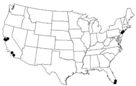
2000 Metropolitan Areas: Sprawl Index 0 to < 25

Figure 4.

2000 Metropolitan Areas: Sprawl Index 75 to 100

The great number of metropolitan areas scoring between 50 and 75 in the Midwest and North East are visible, punctuated by occasional older, larger metropolitan areas scoring below 50 that seem to broadly follow the Interstate 80/90 and 95 corridors. There is a string of metropolitan areas scoring between 50 and 75 along Interstate 5 from California to Washington, with another grouping from Texas to North Dakota. Metropolitan areas scoring between 25 and 50 are found throughout the Pacific Coast and Southwestern parts of the country as well as a cluster in Colorado and South Texas. Most of the large metropolitan areas of the country stand out as scoring between 25 and 50 in contrast to the surrounding smaller metropolitan areas that are more likely to score above 50. Metropolitan areas scoring below 25 are only found on the Atlantic and Pacific coasts in four clusters with two clusters in California and none further north than Central California and New York City.

The distribution and characteristics of the 13 metropolitan areas that had no people living in census tracts with densities higher than 3,500 persons per square mile (sprawl index = 100) were striking. All of these metropolitan areas were in the South and had fewer than 250,000 total people. Only two metropolitan areas containing more than 1,000,000 people were scored above 75, and both of these were in the South (Charlotte and Atlanta).

The comparison with 1990 data (using county-based definitions for New England for both years) showed that there has been a substantial change in the level of sprawl in the United States. In the past decade, sprawl increased in 198 metropolitan areas and decreased in 97. It was unchanged in 21 metropolitan areas, and 11 of these were at 100 in both 1990 and 2000. Large metropolitan areas again had lower levels of sprawl: only 24 saw increased sprawl, and 27 had decreased sprawl. One large metropolitan area was unchanged. Considering all metropolitan areas together, there were almost 16% more metropolitan areas scoring above 75 at the end of the decade but only one net additional metropolitan area scoring below 25. Among large metropolitan areas, the total number of metropolitan areas scoring above 50 decreased by 3. Two metropolitan areas dropped below 25: Ft. Lauderdale and Stockton-Lodi; and one moved above 25: Laredo. The total number of people living in metropolitan areas scoring below 50 grew from 90.5 million to 115.6 million (a 27% increase), whereas the total number of people living in metropolitan areas scoring above 50 grew from 84.2 to 85.0 million (a 0.1% increase). Most net growth has occurred in metropolitan areas with lower sprawl index scores.

DISCUSSION

Surveying metropolitan areas as a whole, it is not surprising that sprawl has become a matter of public debate. More than half the nation's metropolitan areas containing more than 40% of the country's total metropolitan population had a sprawl index greater than 50, indicating that more people lived in lower density census tracts than in higher density tracts. The ratio of metropolitan areas increasing in sprawl versus those decreasing was nearly 2 to 1 over the past decade. The results here are similar to other attempts to measure sprawl, which also found that larger cities tend to be denser and southern cities sprawl more. Others also produced results in keeping with ours that belie the popular conception that Los Angeles is a metropolitan area with low levels of sprawl.

The 1990-2000 growth in the number of people living in less dense census tracts together with the growth in the number of people living in metropolitan areas with index scores less than 50 would at first seem contradictory. However, this may be the result of growth in low-density areas of these larger, denser metropolitan areas. This implies that sprawl is increasing in these metropolitan areas even as they add population because new growth is much less dense than older portions of these metropolitan areas. In contrast, the constant total population of metropolitan areas scoring more than 50 over this time period suggests that population growth in these areas may have pushed some of these metropolitan areas into more dense configurations. The flat growth in metropolitan areas with high sprawl scores also seems contradictory at first given the high rates of growth in the South and in highly sprawled metropolitan areas such as Atlanta. But the high population gains in some sprawled metropolitan areas might have been offset by population losses in other small, highly sprawled metropolitan areas in the Midwest and North East.

The wide distribution of sprawl index scores suggests that sprawl might not be inevitable. Perhaps the collective social, political, and economic decisions along with historical and geographical factors in a metropolitan area can influence the overall level of sprawl. It certainly reveals that there is a large variety of dense and sprawled situations in this country (see Tables 4 and 5).

TABLE 4.

Densest Metropolitan Areas, 2000

Metropolitan Area	State	Sprawl Index
Jersey City	New Jersey	3.94
New York	New York	6.72
Los Angeles	California	10.61
Anaheim	California	14.22
San Jose	California	14.89
Miami	Florida	15.73
San Francisco	California	16.96
Fort Lauderdale	Florida	20.77
Stockton-Lodi	California	21.52
Las Vegas	Nevada	25.54
San Diego	California	26.85
Bergen - Passaic	New Jersey	27.52
Oakland	California	27.78
Chicago	Illinois	30.71
Phoenix	Arizona	31.46
Laredo	Texas	31.50
Denver	Colorado	32.19
New Orleans	Louisiana	32.20
Sacramento	California	32.87
Lincoln	Nebraska	33.88

TABLE 5.

Most Sprawled Metropolitan Areas, 2000

Metropolitan Area	State	Sprawl Index
Hickory–Morganton–Lenoir	North Carolina	100.00
Ocala	Florida	100.00
Myrtle Beach	South Carolina	100.00
Clarksville–Hopkinsville	Tennessee	100.00
Dothan	Alabama	100.00
Florence	South Carolina	100.00
Anniston	Alabama	100.00
Rocky Mount	North Carolina	100.00
Decator	Alabama	100.00
Goldsboro	North Carolina	100.00
Sumter	South Carolina	100.00
Jonesboro	Arkansas	100.00
Sherman–Denison	Texas	100.00
Dover	Delaware	100.00
Greenville–Spartenburg–Anderson	South Carolina	98.76
Barnstable–Yarmouth	Massachusetts	98.23
Augusta–Aiken	Georgia	97.36
Jacksonville	North Carolina	97.32
Gadsen	Alabama	97.27
Johnson City–Kingsport–Bristol	Tennessee	97.21

The great southern sprawl belt warrants further research. Among the possible reasons for the concentration of high levels of sprawl in this region are historical factors such as the tradition of small-scale rural agriculture, cultural values, geographic/climate features, economic factors, demographic trends, land-use policy, or other unknown characteristics. This is the fastest growing region of the country, and the high level and continuing growth of sprawl, even in large metropolitan areas that in other parts of the country tend to be denser, may imply that sprawl will continue to be a public policy issue. The relationship between growth and sprawl is not necessarily directly correlated, however. Las Vegas and Phoenix, two metropolitan areas with high rates of growth, have remained dense.

New England's high number of metropolitan areas scoring above 50 indicates that no region is immune to sprawl. The only metropolitan area outside the South on the list of most sprawled metropolitan areas in 2000 is Barnstable-Yarmouth on Cape Cod. The smaller metropolitan areas of the Midwest have population patterns that indicate sprawl as well. There is a need to better understand why these areas are sprawling.

Similar issues revolve around coastal metropolitan areas. Clearly, there are factors that have resulted in less sprawl along the Atlantic and Pacific coasts. But questions remain as to why the San Francisco, New York, and Miami metropolitan areas have developed at a dense level, whereas Boston and Seattle are less dense. The interaction of geography with urban design, economic, and social trends may influence the level of sprawl.

The high level of sprawl found in smaller metropolitan areas also warrants further research. It may be that low density is a transitory condition for some of these communities and that they will eventually grow into larger, more densely populated areas. On the other hand, this may portend the beginning of the development of a whole new class of very sprawled cities that will ultimately incorporate large portions of the landscape and have potential consequences yet to be studied. The unique intersection of urban form, quality of life, ecosystem health, and development is critical in these metropolitan areas.

It is also important to remember that not all low density or even changes in relative amounts of low density are necessarily deleterious. Lower densities that result from new development that respects wetlands or other environmentally sensitive areas may be considered environmentally beneficial. Clustered housing preserving large tracts of open space is often a goal of environmentally sensitive development. Lowering density to reduce residential overcrowding is also a desirable goal. Further research should examine the relationship between these and other positive policy goals and their net effects on sprawl.

A score indicating a low level of sprawl does not mean the absence of all alleged sprawl-related problems. Miami's growth at its edge threatens the continued health of the Everglades ecosystem (Environmental Economics Symposium Committee 1999), San Jose has struggled to find a way to make its downtown relevant (Hubler 2001; Mathews 1999), and land consumption in Los Angeles is proceeding at a higher rate than population growth (Fulton et al. 2001). Nor do low levels of sprawl guarantee there will be no urban problems. New York City has struggled with abandonment, crime, and all the other problems associated with urban America (Wallace 1988). Furthermore, a low level of sprawl may be associated with an exacerbation of other problems, such as gentrification and the displacement of lower-middle-class and poor people in San Francisco (Zoll 1998). A next step would be to correlate the level of sprawl with a series of potentially related issues such as health outcomes, immigration, racial segregation, housing costs, job availability, environmental policy goals, and land consumption. Another valuable effort would include comparisons to additional past decennial censuses to help determine if sprawl is accelerating or decelerating.

Although the sprawl index is a good measure for discerning varying levels of sprawl in the United States, it is not clear that this index could be used for international comparisons because foreign countries typically have densities far higher than those found in the United States. Raising the threshold levels for the sake of international analysis would reduce differences among U.S. metropolitan areas. Using alternate threshold numbers to accommodate international differences, then, might merely demonstrate that only the United States has cities that sprawl, an unlikely situation. The transferability of this index unaltered across international boundaries remains to be tested.

This sprawl index meets the criteria outlined earlier in this article. This index is measurable and applicable. It uses standardized published data for all metropolitan areas. Although threshold levels can be changed, they were set using objective criteria and represent a reasonable anchor point for the discussion of sprawl. The index is conceptually valid, uses a workable and objective range of values, and is easy to understand and communicate. The efficiency of this measure allows for the identification of metropolitan areas that may warrant more in-depth sophisticated study.

Although the subject of great differences of opinion and debate, sprawl can be quantified. Measuring sprawl reveals great differences among metropolitan areas in the amount of sprawl and important geographical, size, and temporal variation. This suggests that the multifactorial causes of sprawl are complex and remain to be identified and explored singly and together. The social consequences of sprawl also remain to be studied. In particular, the alleged links between urban sprawl and social justice issues of racial segregation, urban poverty, and job availability must be rigorously analyzed so as to promote land-use policies that are environmentally protective and socially just.

Figure 2.

2000 Metropolitan Areas: Sprawl Index 25 to < 50

Figure 3.

2000 Metropolitan Areas: Sprawl Index 50 to < 75

Biography

Russ Lopez, a native of California, received his bachelor of science degree in applied earth sciences from Stanford University and his master of city and regional planning degree from the Kennedy School of Government at Harvard. He worked for 10 years in various positions in Boston and Massachusetts government on housing, community development, and environmental issues. He was the first executive director of the Environmental Diversity Forum, a coalition of environmentalists and community activists advocating for environmental justice issues throughout New England. A longtime volunteer and member of several community-based organizations, he is currently in the doctoral program in environmental health in the School of Public Health at Boston University. Now in the process of completing his dissertation on disparate exposure to air pollution, he is also a lecturer in the Environmental Health Department and a consultant to a number of local and national organizations including the Dorchester Community Collaborative, the Environmental Protection Agency, and the U.S. Department of the Interior. His interests include urban environmental health and the role of the cities and the structure of the built environment in public health outcomes.

H. Patricia Hynes is a professor of environmental health at the Boston University School of Public Health and director of the Urban Environmental Health Initiative where she works on issues of urban environment, feminism, and environmental justice. An environmental engineer, she served as section chief in the Hazardous Waste Division of the U.S. Environmental Protection Agency (EPA) and chief of environmental management at the Massachusetts Port Authority. She is the author of The Recurring Silent Spring (Pergamon, 1989), EarthRight (Prima, 1990), Taking Population out of the Equation: Reformulating I=PAT (Institute on Women and Technology, 1993), and A Patch of Eden: America's Inner-City Gardeners (Chelsea Green, 1996). She has worked with many community-based organizations and serves on the Advisory Board of the Coalition against Trafficking in Women. She is currently codirector of the Lead-Safe Yard Project funded by the EPA and the Healthy Public Housing Initiative in Boston funded by the U.S. Department of Housing and Urban Development (HUD). She also is deputy director of the Prevention Research Center at Boston University School of Public Health funded by the Centers for Disease Control.

Appendix

2000 Sprawl Index Scores

Metropolitan Area	State	Sprawl Index
Abilene	Texas	70.14
Akron	Ohio	68.75
Albany	Georgia	96.13
Albany–Schenectady–Troy	New York	66.79
Albuquerque	New Mexico	46.87
Alexandria	Louisiana	87.68
Allentown–Bethlehem–Easton	Pennsylvania	58.70
Altoona	Pennsylvania	46.13
Amarillo	Texas	51.02
Anaheim	California	14.22
Anchorage	Alaska	44.19
Ann Arbor	Michigan	72.15
Anniston	Alabama	100.00
Appleton–Oshkosh–Neenah	Wisconsin	57.84
Asheville	North Carolina	96.95
Athens	Georgia	83.64
Atlanta	Georgia	80.65
Atlantic–Cape May	New Jersey	63.81
Auburn–Opelika	Georgia	92.59
Augusta–Aiken	Georgia	97.36
Austin–San Marcos	Texas	56.50
Bakersfield	California	47.86
Baltimore	Maryland	47.63
Bangor	Maine	77.36
Barnstable–Yarmouth	Massachusetts	98.23
Baton Rouge	Louisiana	78.46
Beaumont–Port Author	Texas	81.15
Bellingham	Washington	77.75
Benton Harbor	Michigan	94.76
Bergen–Passaic	New Jersey	27.52
Billings	Montana	69.34
Biloxi–Gulfport–Pascagoula	Mississippi	92.46
Binghamton	New York	61.51
Birmingham	Alabama	82.67
Bismarck	North Dakota	52.89
Bloomington	Indiana	63.45
Bloomington–Normal	Illinois	51.08
Boise	Idaho	61.37
Boston	Massachusetts	46.57
Boulder–Longmont	Colorado	50.05
Brazoria	Texas	96.63
Bremerton	Washington	85.46
Bridgeport	Connecticut	54.02
Brockton	Massachusetts	68.18
Brownsville–Harlingen–San Benito	Texas	59.89
Bryan–College Station	Texas	56.74
Buffalo–Niagara Falls	New York	47.69
Burlington	Vermont	72.39
Canton–Massillon	Ohio	72.84
Casper	Wyoming	69.35
Cedar Rapids	Iowa	70.69
Champaign–Urbana	Illinois	51.80
Charleston	West Virginia	83.00
Charleston–North Charleston	South Carolina	85.64
Charlotte–Gastonia–Rock Hill	North Carolina	88.06
Charlottesville	Virginia	61.36
Chattanooga	Tennessee	95.86
Cheyenne	Wyoming	86.99
Chicago	Illinois	30.71
Chico–Paradise	California	74.41
Cincinnati	Ohio	61.64
Clarksville–Hopkinsville	Tennessee	100.00
Cleveland–Lorain–Elyria	Ohio	48.50
Colorado Springs	Colorado	48.14
Columbia	Missouri	79.88
Columbia	South Carolina	87.02
Columbus	Ohio	53.16
Columbus	Georgia	83.60
Corpus Christi	Texas	49.79
Corvallis	Oregon	70.71
Cumberland	Maryland	87.26
Dallas	Texas	44.34
Danbury	Connecticut	84.01
Danville	Virginia	84.91
Davenport–Moline–Rock Island	Iowa	64.06
Dayton–Springfield	Ohio	68.57
Daytona Beach	Florida	84.74
Decatur	Illinois	67.90
Decatur	Alabama	100.00
Denver	Colorado	32.19
Des Moines	Iowa	60.99
Detroit	Michigan	41.76
Dothan	Alabama	100.00
Dover	Delaware	97.21
Dubuque	Iowa	68.39
Duchess County	New York	82.77
Duluth–Superior	Minnesota	68.85
Eau Clair	Wisconsin	74.91
El Paso	Texas	34.18
Elkhart–Goshen	Indiana	87.78
Elmira	New York	64.35
Enid	Oklahoma	83.75
Erie	Pennsylvania	57.01
Eugene–Springfield	Oregon	57.01
Evansville–Henderson	Indiana	73.04
Fargo–Moorhead	North Dakota	56.20
Fayetteville	North Carolina	94.09
Fayetteville–Springdale–Rogers	Arkansas	91.78
Fitchburg–Leominster	Massachusetts	75.20
Flagstaff	Arizona	74.35
Flint	Michigan	74.60
Florence	Alabama	96.13
Florence	South Carolina	100.00
Fort Collins–Loveland	Colorado	51.77
Fort Lauderdale	Florida	20.77
Fort Meyers–Cape Coral	Florida	88.98
Fort Pierce–Port St. Lucie	Florida	91.86
Fort Smith	Arkansas	80.06
Fort Walton Beach	Florida	84.67
Fort Wayne	Indiana	75.49
Fort Worth	Texas	50.95
Fresno	California	40.21
Gadsden	Alabama	97.27
Gainesville	Florida	76.61
Galveston	Texas	71.71
Gary	Indiana	69.51
Glen Falls	New York	70.23
Goldsboro	North Carolina	100.00
Grand Forks	North Dakota	72.47
Grand Junction	Colorado	90.63
Grand Rapids–Muskegon–Holland	Michigan	67.82
Great Falls	Montana	74.08
Greeley	Colorado	43.70
Green Bay	Wisconsin	65.88
Greensboro–Winston-Salem–High Point	North Carolina	91.77
Greenville	North Carolina	75.10
Greenville–Spartanburg–Anderson	South Carolina	98.76
Hagerstown	Maryland	71.93
Hamilton–Middletown	Ohio	78.94
Harrisburg–Lebanon–Carlisle	Pennsylvania	74.63
Hartford	Connecticut	71.46
Hattiesburg	Mississippi	91.92
Hickory–Morganton–Lenoir	North Carolina	100.00
Honolulu	Hawaii	35.46
Houma	Louisiana	84.96
Houston	Texas	45.87
Huntington–Ashland	Kentucky	79.04
Huntsville	Alabama	94.84
Indianapolis	Indiana	71.69
Iowa City	Iowa	45.15
Jackson	Michigan	75.55
Jackson	Mississippi	82.54
Jackson	Tennessee	92.26
Jacksonville	Florida	75.35
Jacksonville	North Carolina	97.32
Jamestown	New York	69.68
Janesville–Beloit	Wisconsin	64.20
Jersey City	New Jersey	3.94
Johnson City–Kingsport–Bristol	Tennessee	97.27
Johnstown	Pennsylvania	77.09
Jonesboro	Arkansas	100.00
Joplin	Missouri	91.79
Kalamazoo–Battle Creek	Michigan	77.67
Kankakee	Illinois	64.74
Kansas City	Missouri	68.05
Kenosha	Wisconsin	53.01
Killeen-Temple	Texas	77.62
Knoxville	Tennessee	94.17
Kokomo	Indiana	81.08
La Crosse	Wisconsin	67.24
Lafayette	Indiana	55.25
Lafayette	Louisiana	91.60
Lake Charles	Louisiana	87.05
Lakeland–Winter Haven	Florida	87.38
Lancaster	Pennsylvania	77.13
Lansing–East Lansing	Michigan	64.68
Laredo	Texas	31.50
Las Cruces	New Mexico	77.35
Las Vegas	Nevada	25.54
Lawrence	Kansas	55.64
Lawrence	Massachusetts	68.47
Lawton	Oklahoma	58.97
Lewiston–Auburn	Maine	70.40
Lexington	Kentucky	57.43
Lima	Ohio	72.92
Lincoln	Nebraska	33.88
Little Rock	Arkansas	85.93
Longview-Marshall	Texas	96.26
Los Angeles	California	10.61
Louisville	Kentucky	61.90
Lowell	Massachusetts	66.61
Lubbock	Texas	39.65
Lynchburg	Virginia	94.78
Macon	Georgia	92.53
Madison	Wisconsin	56.53
Manchester	New Hampshire	67.13
Mansfield	Ohio	77.70
McAllen-Edinburg-Mission	Texas	87.31
Medford-Ashland	Oregon	67.49
Melbourne–Titusville–Palm Bay	Florida	84.38
Memphis	Tennessee	62.78
Merced	California	62.69
Miami	Florida	15.73
Middlesex–Somerset–Hunterdon	New Jersey	50.11
Milwaukee–Waukesha	Wisconsin	49.41
Minneapolis–St. Paul	Minnesota	59.11
Missoula	Montana	62.12
Mobile	Alabama	82.72
Modesto	California	34.84
Monmouth–Ocean	New Jersey	66.34
Monroe	Louisiana	93.11
Montgomery	Alabama	85.65
Muncie	Indiana	71.31
Myrtle Beach	South Carolina	100.00
Napa	California	41.99
Naples	Florida	75.04
Nashua	New Hampshire	79.02
Nashville	Tennessee	79.36
Nassau–Suffolk	New York	34.80
New Bedford	Massachusetts	50.59
New Haven–Meriden	Connecticut	57.64
New London–Norwich	Connecticut	86.72
New Orleans	Louisiana	32.20
New York	New York	6.72
Newark	New Jersey	37.41
Newburgh	New York	77.62
Norfolk–Virginia Beach–Newport News	Virginia	47.42
Oakland	California	27.78
Ocala	Florida	100.00
Odessa-Midland	Texas	53.81
Oklahoma City	Oklahoma	58.15
Olympia	Washington	93.39
Omaha	Nebraska	43.96
Orlando	Florida	64.34
Owensboro	Kentucky	74.78
Oxnard-Ventura	California	34.57
Panama City	Florida	96.86
Parkersburg–Marietta	West Virginia	83.64
Pensacola	Florida	95.71
Peoria–Pekin	Illinois	70.56
Philadelphia	Pennsylvania	43.36
Phoenix	Arizona	31.46
Pine Bluff	Arkansas	91.44
Pittsburgh	Pennsylvania	57.74
Pittsfield	Massachusetts	79.60
Pocatello	Idaho	81.19
Portland	Maine	74.86
Portland-Vancouver	Oregon	40.99
Portsmouth–Rochester	New Hampshire	91.58
Providence–Fall River–Warwick	Rhode Island	56.50
Provo-Orem	Utah	52.12
Pueblo	Colorado	46.53
Punta Gorda	Florida	96.22
Racine	Wisconsin	61.58
Raleigh–Durham–Chapel Hill	North Carolina	81.91
Rapid City	South Dakota	93.72
Reading	Pennsylvania	64.30
Redding	California	90.86
Reno	Nevada	53.60
Richland-Kennewick-Pasco	Washington	76.68
Richmond–Petersburg	Virginia	77.60
Riverside-San Bernardino	California	48.74
Roanoke	Virginia	90.55
Rochester	Minnesota	60.11
Rochester	New York	65.02
Rockford	Illinois	69.57
Rocky Mount	North Carolina	100.00
Sacramento	California	32.89
Saginaw–Bay City–Midland	Michigan	76.15
Salem	Oregon	55.25
Salinas	California	36.01
Salt Lake City–Ogden	Utah	34.80
San Angelo	Texas	78.25
San Antonio	Texas	45.04
San Diego	California	26.85
San Francisco	California	16.96
San Jose	California	14.89
San Luis Obispo	California	71.36
Santa Barbara	California	37.87
Santa Cruz	California	47.95
Santa Fe	New Mexico	63.88
Sarasota–Bradenton	Florida	73.28
Savannah	Georgia	68.35
Scranton–Wilkes Barre–Hazleton	Pennsylvania	61.04
Seattle-Bellevue-Everett	Washington	41.97
Sharon	Pennsylvania	63.82
Sheboygan	Wisconsin	61.38
Sherman-Denison	Texas	100.00
Shreveport–Bossier City	Louisiana	77.27
Sioux City	Iowa	77.60
Sioux Falls	South Dakota	61.06
Sonoma	California	55.44
South Bend	Indiana	60.72
Spokane	Washington	48.05
Springfield	Massachusetts	63.43
Springfield	Illinois	70.87
Springfield	Missouri	83.50
St. Cloud	Minnesota	76.14
St. Joseph	Missouri	65.08
St. Louis	Missouri	57.98
Stamford–Norwalk	Connecticut	54.20
State College	Pennsylvania	51.62
Steubenville–Weirton	Ohio	87.20
Stockton-Lodi	California	21.52
Sumter	South Carolina	100.00
Syracuse	New York	62.85
Tacoma	Washington	61.06
Tallahassee	Florida	78.60
Tampa–St. Petersburg–Clearwater	Florida	50.13
Terre Haute	Indiana	78.87
Texarkana	Texas	92.15
Toledo	Ohio	55.92
Topeka	Kansas	71.67
Trenton	New Jersey	56.13
Tucson	Arizona	46.61
Tulsa	Oklahoma	63.78
Tuscaloosa	Alabama	80.23
Tyler	Texas	86.32
Utica–Rome	New York	70.95
Victoria	Texas	49.19
Vineland–Millville–Bridgeton	New Jersey	66.70
Visalia–Tulare	California	47.70
Waco	Texas	72.58
Washington	District of Columbia	42.45
Waterbury	Connecticut	67.39
Waterloo–Cedar Falls	Iowa	65.22
Wausau	Wisconsin	81.52
West Palm Beach–Boca Raton	Florida	46.86
Wheeling	West Virginia	90.14
Wichita	Kansas	64.91
Wichita Falls	Texas	87.31
Williamsport	Pennsylvania	75.81
Wilmington	North Carolina	92.39
Wilmington–Newark	Delaware	61.78
Worcester	Massachusetts	71.52
Yakima	Washington	67.49
York	Pennsylvania	77.01
Youngstown–Warren	Ohio	77.05
Yuba City	California	62.48
Yuma	Arizona	59.36
New England County metropolitan areas
Bangor	Maine	77.18
Barnstable–Yarmouth	Massachusetts	98.67
Boston–Worceter–Lawrence–Lowell–Broctorn	Massachusetts	55.84
Burlington	Vermont	72.39
Hartford	Connecticut	71.65
Lewiston–Auburn	Maine	70.40
New Haven–Bridgeport–Stamford–Waterbury–Danbury	Connecticut	58.59
New London–Norwich	Connecticut	86.10
Pittsfield	Massachusetts	83.73
Portland	Maine	76.86
Providence–Warwick–Pawtucket	Rhode Island	45.72

REFERENCES

- Beaumont C. How superstore sprawl can harm communities: And what citizens can do about it. National Trust for Historic Preservation; Washington, DC: 1997. [Google Scholar]
- Black T. The economics of sprawl. Urban Land. 1996;55(3):6–52. [Google Scholar]
- Brueckner J. Growth controls and land values in an open city. Land Economics. 1990;66(3):237–48. [Google Scholar]
- Bullard R, Johnson G, Torres A. Sprawl city: Race, politics and planning in Atlanta. Island Press; Washington, DC: 2000. [Google Scholar]
- Burchell R, Shad N, Litokin D, Phillips H, Downs A, Seskin S, Davis J, Moore T, Helton D, Gall M. The costs of sprawl revisited. National Academy Press; Washington, DC: 1998. (TCRP report no. 39). [Google Scholar]
- Coulter P. Measuring inequality: A methodological handbook. Westview; Boulder, CO: 1989. [Google Scholar]
- Downs A. Some realities about sprawl and urban decline. Brookings Institution; Washington, DC: 1999. [Google Scholar]
- Duany A, Plater-Zyberk E, Speck J. Suburban nation. North Point; New York: 2000. [Google Scholar]
- Environmental Economics Symposium Committee . In South Florida, the environment is the economy. Greater Miami Chamber of Commerce; Miami, FL: 1999. [Google Scholar]
- Ewing R. Is Los Angeles-style sprawl desirable? Journal of the American Planning Association. 1997;63(1):107–26. [Google Scholar]
- Firestone D. The new look suburbs: Denser or more far-flung. New York Times. 2001 April 17;:1. [Google Scholar]
- Freeman L. The effects of sprawl on neighborhood social ties: An explanatory analysis. Journal of the American Planning Association. 2001;67(1):69–77. [Google Scholar]
- Fulton W, Pendall R, Nguyen M, Harrison A. Who sprawls most? How growth patterns differ across the U.S. Brookings Institution; Washington, DC: 2001. [Google Scholar]
- Galster G, Hanson R, Woman H, Coleman S, Friebage J. Wrestling sprawl to the ground: Defining and measuring an elusive concept. Fannie Mae; Washington, DC: 2000. [Google Scholar]
- Garreau J. Edge city: Life on the new frontier. Doubleday; New York: 1991. [Google Scholar]
- Glaeser E, Kahn M. Brookings-Wharton Papers on Urban Affairs. Brookings Institution; Washington, DC: 2001. Decentralized employment and the transformation of the American city. [Google Scholar]
- Glaeser E, Kahn M, Chu C. Job sprawl: Employment location in U.S. metropolitan areas. Brookings Institution; Washington, DC: 2001. [Google Scholar]
- Gordon P, Richardson H. Are compact cities a desirable planning goal? Journal of the American Planning Association. 1997;63(1):107–26. [Google Scholar]
- Hayward S. Legends of the sprawl. Policy Review. 1998;91:26–32. [Google Scholar]
- Heim C. Leapfrogging, urban sprawl, and growth management: Phoenix, 1950-2000. American Journal of Economics and Sociology. 2001;60(1):245–83. [Google Scholar]
- Heinlich R, Andersen W. Development at the urban fringe and beyond: Impacts on agriculture and rural land. U.S. Department of Agriculture; Washington, DC: 2001. (ERS agriculture economics report no. 803). [Google Scholar]
- Henderson V, Arindam M. The new urban landscape: Developers and edge cities. Regional Science and Urban Economics. 1996;26:613–43. [Google Scholar]
- Hubler S. San Jose almost arrives, until the tech downturn, the city seemed poised to rival L. A. and San Francisco in influence. Los Angeles Times. 2001 August 14;:A1. [Google Scholar]
- Jackson K. Crabgrass frontier: The suburbanization of the United States. Oxford Univ. Press; New York: 1985. [Google Scholar]
- Johnson M. Environmental impacts of urban sprawl: A survey of the literature and proposed research agenda. Environment and Planning. 2001;33:717–35. [Google Scholar]
- Jordan S, Ross J, Usowski K. U.S. suburbanization in the 1980s. Regional Science and Urban Economics. 1998;28:611–27. doi: 10.1016/s0166-0462(98)00016-7. [DOI] [PubMed] [Google Scholar]
- Kahn M. Does sprawl reduce the black/white housing consumption gap? Housing Policy Debate. 2001;12(1):77–86. [Google Scholar]
- Kline J. Comparing states with and without growth management: Analysis based on indicators with policy implications comment. Land Use Policy. 2000;17:349–55. [Google Scholar]
- Kunstler J. The geography of nowhere. The rise and decline of America's man-made landscape. Simon and Schuster; New York: 1993. [Google Scholar]
- Lehrer U, Milgram R. New (sub)urbanism: Countersprawl or repackaging the product. Capitalism, Nature and Socialism. 1996;7(2):49–62. [Google Scholar]
- Mathews J. The Los Angeles of the north: San Jose's transition from fruit capital to high-tech metropolis. Journal of Urban History. 1999;25(4):459–76. [Google Scholar]
- Mieszkowski P, Mills E. The causes of metropolitan suburbanization. Journal of Economic Perspectives. 1993;7(3):135–47. [Google Scholar]
- Nelson A. Comparing states with and without growth management: Analysis based on indicators with policy implications. Land Use Policy. 1999;16:121–27. [Google Scholar]
- Ohls J, Pines D. Discontinuous urban development and economic efficiency. Land Economics. 1975;3:224–34. [Google Scholar]
- Parsons Brinckerhoff Quade and Douglas, Inc. Transit, urban form, and the built environment: A summary of knowledge. Vol. 1. National Academy Press; Washington, DC: 1996. Transit and urban form. [Google Scholar]
- Popenoe D. Urban sprawl: Some neglected sociological considerations. Sociology and Social Research. 1979;63(2):255–68. [Google Scholar]
- Ross C, Dunning A. Land use transportation interaction: An examination of the 1995 NPTS data. Report prepared for the U.S. Department of Transportation, Federal Highway Administration. 1997 [Google Scholar]
- Sheehan M. City limits: Putting the breaks on sprawl. Worldwatch Institute; Washington, DC: 2001. (Worldwatch paper no. 156). [Google Scholar]
- Wallace R. A synergism of plagues: Planned shrinkage, contagious housing destruction and AIDS in the Bronx. Environmental Research. 1988;47(1):1–33. doi: 10.1016/s0013-9351(88)80018-5. [DOI] [PubMed] [Google Scholar]
- Zoll D. The economic cleansing of San Francisco. San Francisco Bay Guardian. 1998 October 7;:1. [Google Scholar]