Abstract
Systems Biology requires that biological modelling is scaled up from small components to system level. This can produce exceedingly complex models, which obscure understanding rather than facilitate it. The successful use of highly simplified models would resolve many of the current problems faced in Systems Biology. This paper questions whether the conclusions of simple mathematical models of biological systems are trustworthy. The simplification of a specific model of calcium oscillations in hepatocytes is examined in detail, and the conclusions drawn from this scrutiny generalized. We formalize our choice of simplification approach through the use of functional ‘building blocks’. A collection of models is constructed, each a progressively more simplified version of a well-understood model. The limiting model is a piecewise linear model that can be solved analytically.
We find that, as expected, in many cases the simpler models produce incorrect results. However, when we make a sensitivity analysis, examining which aspects of the behaviour of the system are controlled by which parameters, the conclusions of the simple model often agree with those of the richer model. The hypothesis that the simplified model retains no information about the real sensitivities of the unsimplified model can be very strongly ruled out by treating the simplification process as a pseudo-random perturbation on the true sensitivity data. We conclude that sensitivity analysis is, therefore, of great importance to the analysis of simple mathematical models in biology. Our comparisons reveal which results of the sensitivity analysis regarding calcium oscillations in hepatocytes are robust to the simplifications necessarily involved in mathematical modelling. For example, we find that if a treatment is observed to strongly decrease the period of the oscillations while increasing the proportion of the cycle during which cellular calcium concentrations are rising, without affecting the inter-spike or maximum calcium concentrations, then it is likely that the treatment is acting on the plasma membrane calcium pump.
Keywords: modelling, simplification, hepatocytes
1. Introduction
Biological phenomena can rarely be understood by examining only a few molecules or genes because they are the products of large networks of interacting components. These systems often are of sufficient size and complexity that their behaviour cannot be understood by qualitative reasoning alone. The emerging field of Systems Biology seeks to use mathematical and computational modelling to gain an understanding of complex biological processes at a whole-system scale.
The most obvious methodology is the construction of extremely large, detailed models of biological systems, taking into account all the known biological information. Such constructs may perform as simulations, reproducing the behaviour of the system with high fidelity. This approach imposes an enormous data-gathering burden, but has proved relatively successful in some contexts when it is coupled with very large, dedicated, high-throughput experimental work (e.g. imaging (Nelson et al. 2002) or metabolomics (Maher et al. 2003)). It can also work in contexts such as electrophysiology where there exists a long, detailed literature of model building (Hodgkin & Huxley 1952) with gradual and well-supported increases in model complexity (Noble 2002). However, such models are profligate with modelling effort and/or require a huge experimental commitment, often at large expense extended over long time-scales.
An alternative strategy is to simplify the system, leaving out detail believed to be functionally less important. If we model the network structure correctly, then it should be possible to say something useful about system behaviour without modelling all the molecular details.
Systems Biology seeks to work with larger and more complex models, but the lessons of earlier studies are still of great importance. Simplified models will not provide precise simulations of the biology and they will never replace detailed experimentation. However, simple models can assist in pointing out lines for further experimentation and can aid understanding. Models that sometimes give incorrect answers, but nevertheless perform significantly better than chance in predicting the outcome of some experiment, could be extremely valuable in, for example, the early stages of drug discovery.
On the other hand, piecemeal simplification does not scale well to the construction of complex composite models required for Systems Biology. Instead, we can try to use a common simplification methodology on all parts of the system, a more naive approach, but one with better scaling properties. Such an approach can be called ‘systematic simplification’.
This approach has been applied successfully to the modelling of metabolic networks, where useful models have been constructed using only the stoichiometries of the reactions, neglecting all the rate- and equilibrium constants, for example through flux balance analysis (Edwards et al. 2001; Holzhutter 2004) or elementary mode analysis (Schuster et al. 1999).
Another systematic simplification methodology has been variously termed ‘extreme nonlinearity’, ‘logical’, or ‘binary’ network models, or ‘threshold’ models. In this approach, the system is treated as a digital network, with each element's contribution being either on or off. Such models have a long history (Kauffman 1969), and analytic techniques exploiting this discrete logical structure have been developed (Glass & Kauffman 1972, 1973; Kaufman et al. 1985; Kaufman & Thomas 1987; Snoussi & Thomas 1993; Thomas 1998; Thomas & Kaufman 2001).
Our systematic simplification approach constructs models using a set of simple nonlinear elements corresponding to common system control elements such as switches, linear decays, convergent pathways and saturations. Each building block is a ‘smoothed’ form of some logical element. Logical models can be recovered as a mathematical limit of modelling with such elements. In this limit, the models become piecewise linear, and can be analysed analytically. Here, we use only one building block—a simple Hill function is used wherever switch-like behaviour occurs within the system. The aim of our procedure is to reach a point where algebraic analysis is possible, while ensuring that nothing of significance is lost. If significant dynamical properties are lost, the nature of any bifurcations that occur as the degree of nonlinearity (Hill exponent) is increased should reveal the reason. Note that while other authors have compared the results of logical models with continuous equivalents (Glass & Kauffman 1972; Kaufman & Thomas 1987), we present a systematic comparison involving a detailed analysis of how the model behaviour changes as the logical limit is gradually obtained.
Models of the reaction dynamics of complex networks are likely to involve a number of reactions with very different response functions. Can we successfully represent them all using elements such as the Hill function? Even if they can be represented using the same functional forms, they will have a variety of parameter values, such as the associated Hill exponents. Can this variety be abstracted away and still leave a useful model? More generally, can models be systematically simplified in a way that renders them analytically tractable, but retains the key qualitative dynamical features exhibited by models based on more precise specifications of known molecular mechanisms?
The present work grew out of efforts to construct a model of the blood glucose control system of the liver. Hepatocytes release glucose by breaking down glycogen stored within them (glycogenolysis) in response to binding of glucagon or adrenaline to surface membrane receptors. The molecular systems involved in this pathway are complex. The full model system comprises three hormone receptors (for noradrenaline, glucagon and insulin) and their associated membrane proteins, three second messengers (calcium, IP3 and cAMP) and their effects, two kinase-cascades controlling glycogen phosphorylase and glycogen synthase and the import and export of glucose (Bollen et al. 1998; King 2005).
Using our approach, simple models of such complex systems can be constructed relatively easily. However, in this article, we focus on general questions of model simplification for Systems Biology, rather than presenting scientific conclusions based on our model of liver glucohomeostasis. We wish to understand how systematic simplification corrupts a model's predictions and which model predictions survive the simplification process uncorrupted. To this end, we focus on a submodel involving only the most well-understood part of the system, that is responsible for transduction of the signal for glycogen breakdown from the messenger species inositol trisphosphate (IP3) to cytosolic calcium ions (Ca2+). Calcium levels in hepatocytes oscillate in response to glucagon and adrenaline. These oscillations are triggered by increasing levels of IP3, and the resulting alterations in calcium concentration induce glycogen breakdown. We choose to focus on this system component because of its rich experimental and modelling history (for a review, see Schuster et al. 2002).
Here, we examine the impact of simplification on mathematical models by using as exemplar a model of these oscillations by Thomas Höfer (Höfer 1999). The resulting limiting simplification is a piecewise linear model of calcium oscillations. This is by no means the first such model, see Sneyd et al. (1993). However, we use the technique of sensitivity analysis, also called control analysis (Saltelli et al. 2000), whereby the degree of control each model parameter has on model output is examined to assess the effect of the systematic simplification procedure. This technique is well established in mathematical modelling in many fields, including biology. It has been particularly important in considering metabolism (Hofmeyr 1995; Heinrich & Schuster 1996; Fell 1997). For an example of its application to a model of glycogenolysis, see Lambeth & Kushmeric (2002). Here, we examine parameter sensitivity by developing a statistical model to show that, although the simplified model often gets the detailed quantitative behaviour of the system wrong, it can perform well in predicting which parameters have significant control over various system properties.
2. Simplification procedure
2.1 The Hill function
Many elements of biological systems have switch-like relationships with one another. For example, a gradual change in the concentration of one species E can produce a relatively sudden change in another species. We can describe these using a sigmoidal response function Θn, usually called a Hill function:
| (2.1) |
The level e of E required for 50% of the maximum response, is called the threshold value. We call n the Hill exponent of the response. In the limit, as n becomes very large, Θn becomes a switch function with threshold e
| (2.2) |
with H(x)=0 for x<0, H(x)=1 for x>0. The shapes of these Hill-function responses for high and low values of n are illustrated in figure 1.
Figure 1.
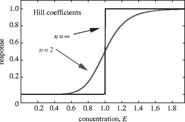
The Hill function for the indicated values of the Hill exponent n.
2.2 Simplifying mechanistic models
The simplification approach we use proceeds in several stages.
Begin with the target model that we wish to simplify systematically.
For each ‘switch-like behaviour’ in the target model—this assignment being based on an understanding of the underlying biology—formulate a submodel with the behaviour represented by a Hill function, selected so that the new response is as close as possible to the given mechanistic response. The result is a Hill function model.
Replace all of the resulting Hill exponents by a common value n, usually 2 or 3, selected for minimal change to model behaviour. The result is a common Hill exponent model.
Gradually increase the common Hill exponent in the common Hill exponent model, examining the changes in model behaviour as the parameter increases.
Take the limit n→∞, to form a threshold model, in which all responses are perfect switches.
Analyse the threshold model, which is a piecewise linear, to obtain analytical results for the key features of its behaviour, which constitute an analytical model.
This scheme can be applied to other functional forms which also have some parameter n, parameterizing their degree of nonlinearity such that they become piecewise linear as n→∞. For example, the fuzzy minimum
| (2.3) |
which has the property that , the minimum of the non-negative quantities x and y. This construction can be used, for example, to model saturating hormone reactions, which proceed at a rate controlled by the substrate concentration only when this is below the enzyme's Michaelis constant.
There are multiple choices of function with the appropriate limiting behaviour, for example, for a softened switch, instead of a Hill function, one could use an error function, as in Glass & Kauffman (1972).
3. Model definitions
3.1 Models of calcium oscillations
We use models of calcium oscillations to illustrate the simplification procedure. The models we consider include two stores of calcium and two corresponding dynamical variables, the concentration of calcium in the cytoplasm, denoted C, and in the endoplasmic reticulum (ER), denoted E. An alternative parameterization uses C and the total cellular calcium measured in units of equivalent cytoplasmic concentration, Z=C+vE, where v is the effective ratio of the ER space to that of the cytoplasm, taking into account calcium buffering capacity. These are treated as homogeneous variables, with diffusion of calcium through the intracellular media considered fast. Calcium moves into and out of the cell, and across the ER–cytosol boundary. Oscillation occurs as calcium moves between these two pools. Models in this class treat the level of IP3, here denoted P(t), as an external driving function. The level of calcium does not feed back into the level of IP3. A model consists of a pair of differential equations
| (3.1) |
| (3.2) |
where JER is the net rate of flow of calcium between the ER and the cytosol and JPM is the net rate of flow of calcium between the cytosol and the external medium (PM denotes plasma membrane). These are often separated into positive and negative parts, as they represent different biological processes
| (3.3) |
with X=(ER, PM).
It is assumed that JPM is a function only of C, P(t) and the external concentration of calcium S(t). Similarly, JER is a function only of C, E and P(t). These functions are also dependent on parameters, collectively denoted as k={ki}, such as reaction rates, which describe the molecular mechanisms involved in the movement of calcium.
Calcium pumps on the ER and plasma membranes, called the SERCA (Sarco/endoplasmic reticulum calcium atp-ase) and PMCA (plasma membrane calcium atp-ase), respectively, account for JER,out and JPM,out. These have usually been modelled as saturating, monotonically increasing functions of cytosolic calcium concentration, although dependence on external or ER calcium concentration can also be included. Calcium channels on the plasma membrane account for JPM,in, which is typically modelled as a monotonically increasing, saturating function of P, and also may depend on S. Finally, calcium release from the ER is known to be promoted by IP3, and by moderate levels of cytosolic calcium (calcium-induced calcium release, CICR), but inhibited by high concentrations of cytosolic calcium. Thus, JER,in has been modelled as a monotonically increasing, saturating function of P and a peaked function of C (Bezprozvanny et al. 1991; Keener & Sneyd 1998; Taylor 1998). For zero P and zero C, the ‘in’ flows typically show some small leak. Thus, in the absence of stimulation by hormone, there are resting equilibrium values of C and E.
3.2 Systematic simplification
The target model for systematic simplification (§2.2) is taken from Höfer (1999). When the target model already expresses switch-like behaviours as Hill functions, it is necessary only to rewrite these using our Θ notation, to make this explicit. Doing so we obtain a representation of the target model for this paper:
| (3.4) |
| (3.5) |
| (3.6) |
| (3.7) |
| (3.8) |
| (3.9) |
The parameter values given in Hofer (1999) were selected to fit observed patterns of oscillations, and are listed in table 1.
Table 1.
The parameters for the target model and for the Hill function model giving the best fit to the target model. (Units are μM for concentration and seconds for time.)
| symbol | meaning | value | value in simplified model |
|---|---|---|---|
| kMC | maximum flow rate for IP3 sensitive membrane calcium channels | 0.08 | 0.08 |
| kMP | maximum flow rate for PMCA | 0.072 | 0.072 |
| kEC | maximum flow rate for CICR | 80.0 | 2.0 |
| kEP | maximum flow rate for SERCA | 18.0 | 18.0 |
| CEC,+ | opening threshold calcium for CICR | 0.4 | 0.26 |
| CEC,− | closing threshold calcium for CICR | 0.4 | 0.65 |
| pEC | threshold IP3 for CICR | 0.2 | 0.45 |
| cEP | threshold calcium for PMCA | 0.12 | 0.12 |
| pMC | threshold IP3 for membrane channels | 4.0 | 4.0 |
| cMP | threshold cytosolic calcium for SERCA | 0.12 | 0.26 |
| lMC | leak in membrane channel, as a fraction of maximum flow | 0.05 | 0.05 |
| lEC | leak in CICR | 0.02 | 0.02 |
| v | effective volume ratio cytoplasm/ER | 10.0 | 10.0 |
| d1 | fitting parameter in target model | 0.3 | n/a |
| d3 | fitting parameter in target model | 0.2 | n/a |
This model is already close to being expressed using only Hill functions. Only JER,in needs modification. A good fit to JER,in, over a wide range of values of C and P, can be found using the expression
| (3.10) |
in place of equation (3.8), with appropriate values of lEC, pEC, cEC,+ and cEC,−. The two functions differ by less than 10% over a wide range of P (from 0 to 2 μM), despite removal of the threshold crosstalk. We shall see that the selection of n=2 as a common Hill exponent also has little effect on the conclusions. The parameters, their meanings and values, used to obtain the best fit of JER,in, are shown in table 1. These substitutions result in the Hill function model (§2.2).
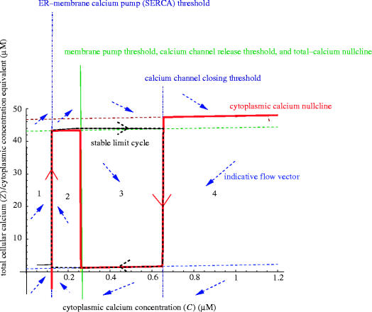
The Hill exponent n is increased and produces a threshold model in the limit n→∞. However, if this is tried without further modification of the model, the system ceases to oscillate for n>5. A simple phase-plane analysis reveals that oscillations occur when the C nullcline has negative slope where it crosses the Z nullcline (C=cMP). For infinite n, this occurs only at C=cEC,+. Thus, a threshold model cannot possibly answer the question ‘what range of values of the PMCA threshold result in stable oscillations?’, because the answer depends directly on the degree of sharpness of the opening of the ER calcium channel. This is a question that cannot be answered in the threshold limit, but, nevertheless, we can modify the model so that oscillations continue to exist in the large n limit. The required modification reduces the number of parameters of the threshold model by one, equating the values of cMP and cEC,+. This does not have a significant effect on other properties of the model. The resulting threshold model is solved to obtain the analytical model (see appendix A).
4. Methodology for comparison of models
4.1 Dynamical features
Models have large ranges of possible behaviours, corresponding to different choices for the parameters and for the input functions. The size of the problem can be reduced by studying the behaviour of the models for a particular choice of the input functions corresponding to some particular virtual experiment. Our choice is to set S(t) to a constant s, and P(t) to a constant p during the simulation, but assume in our initial conditions that the system has spent a long time prior to the simulation with P(t)=0, thus the simulation begins with a transient response to the addition of IP3.
To focus on a finite set of aspects of the behaviour of the variables of interest, we consider a number of observables associated with typical oscillations: the period of oscillations; the fraction of the period on the upstroke of the oscillations; and the minimum and maximum values of the cytoplasmic calcium concentration. These are potentially experimentally measurable quantities, and are shown in figure 2 and listed in table 2. For numerical work, algorithms for locating the special points associated with these observables must be specified. Our implementation uses interpolated uneven time-series. Note that we make these choices to reduce the size of the problem to a manageable level—it is clear that other observables and virtual experiments could be chosen.
Figure 2.
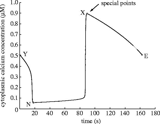
The points indicated are those used to define observables, chosen to show important features of a typical behaviour in the virtual experiment. Note that the observables are defined on a typical cycle of the oscillatory behaviour. We denote the (time, value) pair of a particular special point Y as (tY, CY).
Table 2.
The chosen observables, defined using the special points from figure 2. (The (time, value) pair of a point Y is denoted as (tY, CY).)
| name | symbol | definition |
|---|---|---|
| period | Π | tE−tY |
| fraction rising | Ψ | (tX−tN)/(tE−tY) |
| maximum | M | CX |
| minimum | N | CN |
4.2 Comparative sensitivity analysis
We examine our models using sensitivity analysis (Heinrich & Schuster 1996; Fell 1997; Saltelli et al. 2000). For observables ωi and parameters ki, define the fractional sensitivity of ωi to kj by
| (4.1) |
evaluated at a specified operating point, a point in parameter space. We shall compare the values of these sensitivities obtained from different models. Thus, we must select a pair of operating points, one for each model. A naive choice of operating points in a pair of models' parameter spaces is to use identical numerical values for parameters which are believed to correspond to the same biological aspects. Since the behaviours of the models are different, and the numbers and definitions of parameters of those models may be different, one may ask what justifies such a choice. That we have only tenuous a priori reasons to believe that the two models will agree, given this choice, is not something which undermines our approach, but rather, is an important motivation for making such a study as this one. We are seeking a posteriori justification for this choice, which, if it works, significantly decreases the difficulties involved in simplification for Systems Biology. Any other choices made in the selection of operating point, for example the setting of two thresholds the same in §3.2, will also be justified if the results from the models are similar.
4.3 Statistical comparative sensitivity analysis
The central question to be addressed in the comparative sensitivity analysis is: to what extent is information contained in the parameter sensitivities of model A retained in the sensitivities of model B? Although both models are deterministic, and hence any agreement/disagreement between them could be explained by a careful analysis of the underlying dynamics, nevertheless we treat this as a statistical question, namely: Is the model B sensitivity matrix, B=(bij), significantly different from a ‘random’ perturbation (in a sense to be made precise) of the target model sensitivity matrix, A=(aij)? Thus, the model B sensitivities are viewed as sample data from a random variable B, and we would like to draw conclusions regarding its distribution from this sample.
To do this prior assumptions are necessary. First, we assume that the elements of B are independent, identically distributed (i.i.d), conditional on the corresponding value A (i.e. if aij=akl, then Bij and Bkl are i.i.d.). This allows aggregation of the elements of A and B into vectors a and b, yielding a sample of sufficient size to test hypotheses.
One choice of statistical approach is to use a linear correlation coefficient, C. Using this approach, we expect C=1 when a=b, and C=0 when the two are independent. Thus, increasing values of C measure increasing sensitivity alignment between the two models.
4.3.1 Logical sensitivities
It is often the case that we speak of a treatment as having either a significant or an insignificant effect on the result of some assay of a biological system. To enable our analysis to make contact with this intuition, we formally define ‘large’ and ‘small’ sensitivity using some (arbitrary) cutoff Λ. Thus, for a sensitivity σ, define the associated logical sensitivity, σΛ, by: σΛ=1 (large) if |σ|>Λ; and σΛ=0 (small) if |σ|≤Λ. Clearly, if Λ is chosen too small, then every sensitivity will be large, and if Λ is chosen too large, then every sensitivity will be small. However, in general we expect to find a range of values of Λ in which useful information is retained in the σΛ. A danger in this method is that an element of a may be large and positive, but the corresponding element of b large and negative. We shall see from our results that this does not occur in practice.
Let the total number of elements in the vectors aΛ and bΛ be n. A true positive occurs when (i.e. both are large), with similar definitions for false positives (large in B, small in A), true negatives (small in A and B) and false negatives (large in A, small in B). Denote the total numbers of these as, respectively, (t, f, h, c). We also denote the total number of agreements between aΛ and bΛ as r=t+c, and the total number of ones in aΛ as a and in bΛ as b=t+f.
We can create non-parametric hypothesis tests using logical sensitivities. Given the independence assumptions concerning the distribution of the random variable B, it follows that all the information in bΛ about this distribution is contained in t and h (or any other choice of two of the quantities (t, f, h, c)). Denote by T, H the random variables of which t, h are samples. The most general statistical model for their distribution is that they are binomially distributed, with probabilities p and q, and sample sizes a and n−a.
The (null) hypothesis that BΛ is independent of aΛ, i.e. that the results of the simplified model have nothing to do with those of the more reliable model, can then be shown to be (see appendix C). Since H0 is one-dimensional, we need a conditional test, and one can show that it is appropriate to condition on b (see appendix D). The distribution of T given H0 and a value of b is hypergeometric (Feller 1968), and conditional tests for the one-sided alternative, , can, therefore, be constructed. This is the alternative that BΛ is (positively) dependent on aΛ. Thus, if we reject H0 in favour of HA, we conclude that the logical sensitivities obtained from model B retain a significant amount of information about the logical sensitivities of model A.
Our results show that this method is robust with respect to the arbitrary choice of Λ over the range in which there is some discrimination between degrees of control. We can choose also whether to normalize the sensitivities of a given observable with respect to its average absolute value over all parameters, so that Λ is comparable across observables. Our conclusions are also robust to this choice.
4.4 Aggregate results
The effects on the observables of the early stages of the simplification are plotted in figure 3, and of the gradual increase in the Hill exponent in figure 4. The results of the sensitivity analysis as a function of the sensitivity threshold Λ are plotted in figure 5. Finally, a summary of all the statistical measures used is shown in figure 6.
Figure 3.

The values of the observables, divided by those for the target model, for the indicated models. Note that the predictions of the models for each observable are comparable, with the exception that, on increasing the Hill exponent n from 2 to 3, the period changes significantly.
Figure 4.
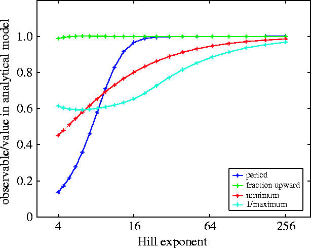
The values of the four observables, divided by those calculated using the analytical model, as functions of the common Hill exponent. The absolute values of the observables at the left-hand side of the figure (n=4) are close to those of the unsimplified model. Note that as n increases, the disagreement with the unsimplified model becomes worse. Note also that the analytical model is a very good approximation to the common Hill exponent model for large n, since for large n, we see the values approaching unity.
Figure 5.
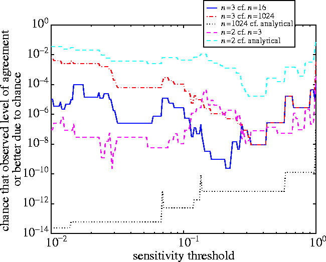
The results of a sensitivity analysis comparison between the common Hill exponent models for n=2, 3, 16, 1024 and for the analytical model. Sensitivities were normalized so that Λ is comparable across observables.
Figure 6.

The full set of comparisons between common Hill exponent models with n=2, 3, 16, 1024, and of each with the analytical model, with a baseline (random) dataset, using all five comparison methods. Λ is the threshold for control to be considered large. P is the P-value for the test of the hypothesis that the logical sensitivities in the two models are independent. In the bottom frame, C is the correlation coefficient. The measures all agree that the simplified models do much better than chance in predicting the sensitivity of less simplified models, and that the loss of correlation between models agrees with intuitive notions of distance in the one-dimensional simplification-space parameterized by n, in that n=2 and n=3 compare well, as do n=1024 and the analytical model.
4.5 Detailed results
In this section, we make a detailed survey of the sensitivity results for two of the models, a less simplified model (A) the common Hill exponent model with n=2 and our most simplified model (B) the analytical model.
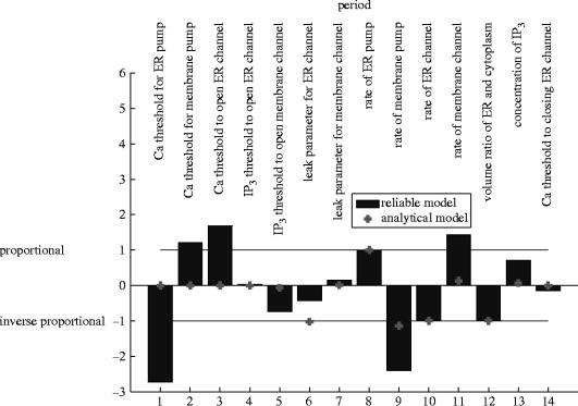
4.5.1 Period
Both models agree that the period is proportional to the rate of the ER pump, inversely proportional to the rate of the ER channel and inversely proportional to the volume ratio of the ER and the cytoplasm (figure 7).
Figure 7.
Sensitivities of the period to the parameters, for the n=2 model and the analytical model.
The models agree that the period is sensitive to the rate of leaking from the CICR channel and the rate at which calcium is pumped out of the membrane. However, in model B, these are both inverse proportionalities, while in model A the dependence is somewhat weaker than inverse proportionality in the former case, and somewhat stronger in the latter.
Model B predicts only weak sensitivity of the period to the current concentration of IP3(+) or the IP3 threshold to open the membrane channel (−). Model A predicts moderate sensitivities. The signs in brackets indicate whether an increase in the parameter increases the observable (+) or decreases it (−).
Model B predicts that the period is slightly increased when the rate of flow of the membrane calcium channel is increased, while A predicts that they are approximately proportional.
Model B completely fails to correctly predict the control on the period of the threshold values for calcium to activate the membrane pump (+), open the CICR channel (+) or activate the ER pump (−) found by model A.
Finally, both models agree that the IP3 threshold to open the ER channel, the leak parameter on the membrane channel and the threshold for calcium to close the ER channel have very little effect on the period.
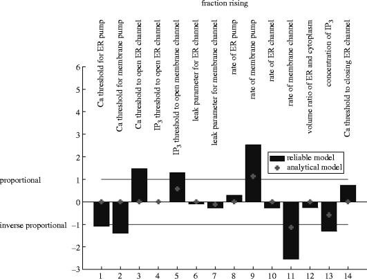
4.5.2 Fraction rising
The models predict this observable as strongly controlled by the rate of the membrane pump (+), the rate of the membrane channel (−), somewhat controlled by the threshold value for IP3 to open the membrane channel (+) and the current level of IP3(−), and weakly controlled by the rate of leaking in the membrane channel (−) (figure 8). In all four cases, the amount of control predicted by model B is smaller than that predicted by model A.
Figure 8.
Sensitivities of the proportion of the cycle spent rising to the parameters, for the n=2 model and the analytical model.
However, the fraction rising is also moderately controlled by the thresholds for calcium to open the ER (−) and membrane pumps (−) or the ER channel (+) or to close the ER channel (+). Model B misses these.
The remaining parameters have little effect or no effect in model A, and no effect in model B.
4.5.3 Minimum and maximum
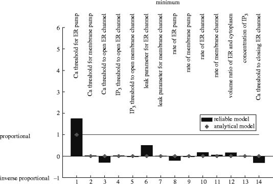
The basal level of calcium during the cycle is confirmed in both models to be almost totally controlled by the threshold for calcium to open the ER pump—exact proportionality in model B, somewhat stronger than proportionality in model A (figures 9 and 10).
Figure 9.
Sensitivities of the minimum calcium to the parameters, for the n=2 model and the analytical model.
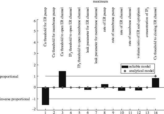
Figure 10.
Sensitivities of the maximum calcium to the parameters, for the n=2 model and the analytical model.
Model A also predicts small amounts of control of the minimum by the threshold for calcium to open the ER channel, the rate of leaking in the ER channel, and the threshold for calcium to close the ER channel, which are missed by model B.
The height of the calcium spike is predicted by both models to be proportional to the threshold for calcium to close the ER channel. (Exact proportionality in model B, approximate in model A.)
Model A also predicts that the maximum is strongly controlled by the threshold value for calcium to open the ER pump (−) and channel (+), which are missed in model B.
5. Conclusions
In carrying out the simplification procedure described in §2.2, we first noticed that our chosen target model, which was not specifically constructed with simplification in mind, was already close to being expressed in terms of building blocks suitable for our procedure. Only one element of the model needed to be changed, and this resulted in a Hill function model which closely matched the target model. This suggests that the loss of freedom suffered by restriction to a finite set of building blocks should not hugely reduce the scope of phenomena we can model.
The early stages of the simplification procedure were quantitatively successful. However, taking the common Hill exponent to high values resulted in significant disagreement between the models. We thus conclude that it is not appropriate to use such highly simplified models as simulations.
However, the models agree better when used for sensitivity analysis. This is observed whether we make an aggregate statistical comparison or a detailed element-by-element study. Our sensitivity analysis thus suggests that highly simplified models can usefully predict which molecular properties within a system might have significant effects on system behaviours. We suggest that the results of such an analysis may be quickly used to analyse experimental results in the light of a model. For example, from our results, one can conclude that if a treatment is observed to strongly decrease the period of the oscillations while increasing the proportion of the cycle during which cellular calcium concentrations are rising, without effecting the inter-spike or maximum calcium concentrations, then the PMCA membrane pump should be considered a likely point of action of the treatment.
Detailed modelling with simulation as its goal carries a heavy data collection price. This paper demonstrates that models constructed using severe simplifications can describe some aspects of system behaviour well, but produce poor results when treated naively as simulations. In particular, simplified models are amenable to analytic treatment and do better than chance at predicting which aspects of the system behaviour are controlled by which parameters.
Using model ‘building blocks’ that reflect the logical properties of a biological network allows models of large, complex systems to be constructed rapidly and efficiently. Where components of a simplified model prove to be inadequate, these can be identified and replaced by a more detailed construction to make the whole system model more realistic.
As Systems Biology develops as a discipline, computational models will not only provide simulations, but also understanding, and will guide experimentation. The demonstration here that even a highly simplified model can reveal useful information about, and insight into, system behaviour should encourage biologists to consider constructing simple models. The systematic simplification methodology we have described, associated with a building-blocks approach to model building, reduces the difficulties associated with generating, and with obtaining significant insight from, large, complex models of whole biological systems.
Acknowledgements
This work was funded by a Beacon Project grant from the Department of Trade and Industry. We thank Prof. Jonathan Ashmore, Prof. Anthony Finkelstein, Dr Peter Saffrey and Ofer Margoninski for useful comments and discussion.
Appendix A. The analytical model
Explicit results for the flow in each segment (patch of the phase plane bounded by the discontinuities in the flow) can be obtained from the threshold model, because it is piecewise linear. For fixed IP3 levels, there are four ranges of calcium, within each of which the system of equations is linear, due to the four thresholds for calcium (cEC,+, cMP, cEP, cEC,−), two of which are the same. In each of the regions, the flow takes the form
where Z=vE+C. The terms μC, αCC, αCZ and μZ can be expressed simply as functions of the parameters in each of the sections. The definitions of the four regions of the phase plane, within each of which this system is linear are
Thus, writing the value of μZ in region i as μZ,i we have
We can obtain a full solution by using the analytic solution to the above linear ordinary differential equations (ODEs) in each patch, and then solving the return equations for the time at which the solution reaches a patch boundary. In the case of oscillatory behaviour, this generates a return map to each of the patch boundaries, the fixed point of which locates the limit cycle. The return equations are transcendental, of the form et+mt=c, the solution to which is given in terms of a special function. However, for our parameter values, C-flow is always rapid except from a narrow region very close to the C-nullclines. (Note the limit cycle is almost horizontal in patches 2 and 3 of figure 11.) The extremal points of the trajectories, therefore, can be found in a simpler way by solving for the intersection points of the nullclines with the patch boundaries, and the period is controlled by μZ: the slow motion in Z moving between the extremal values of Z takes up almost all of the cycle, the motion in C being fast. Thus, we can obtain a simpler analytical model using this approximation for the period by neglecting the time taken for fast motion in C. We obtain simple results for the amplitudes in Z and C and the period of the oscillation. Notation for the four observables is given in table 2.
where MZ and NZ are the maximum and minimum values of Z, which are not observables because Z is not observable. Note that although this is a threshold-limit analysis, the non-limiting soft Hill forms for the parametric dependence on P have been retained. Also note that, with our sign conventions, μZ,3 and μZ,4 are negative, corresponding to the regions where Z is falling.
Figure 11.
The phase plane of the threshold model. The dashed rectangle is the stable limit cycle, the thick sawtooth-shaped line is the cytoplasmic calcium (C) nullcline. Typical flow directions in each of the regions are indicated by arrows.
Appendix B. Well-definedness of the ODE system
One may worry that our threshold model has right-hand sides sufficiently discontinuous to lead to non-unique solutions of the ODE system. However, μZ is single valued on those patch boundaries where dC/dt changes sign, meaning that the threshold limit ODE system is well defined. There are boundaries where μZ is non-single valued, for example, when C=cMP, but these do not occur where dC/dt also changes sign, boundaries where the trajectory ‘sticks’. In other words, the phase-particle velocity is single valued except for infinitesimal moments of time, so there is no problem with solution uniqueness.
Appendix C. Independence of bΛ from aΛ
is independent of if and only if
This occurs if and only if
and (equivalently)
Thus, the condition for to be independent of is p+q=1. This is our null hypothesis H0.
Appendix D. The significance of the agreement between aΛ and bΛ
We seek to construct a test for . Consider
| (D1) |
But
| (D2) |
So
| (D 3) |
| (D4) |
| (D 5) |
where the denominator is evaluated by noting b is binomially distributed under H0, or by using the normalizing identity for the hypergeometric distribution. Note that in equation (D 3), the probability depends on p only through b, so b is the efficient estimator for p, given H0, and is, thus, the appropriate quantity to condition on for the test. The probabilities obtained from equation (D 5), of obtaining the observed value of t given b, a and n, thus form the P-values for our conditional test.
References
- Bezprozvanny I, Watras J, Ehrlich B.E. Bell-shaped calcium–response curves of Ins(1,4,5)P3- and calcium-gated channels from endoplasmic reticulum of cerebellum. Nature. 1991;351:751–754. doi: 10.1038/351751a0. [DOI] [PubMed] [Google Scholar]
- Bollen M, Keppens S, Stalmans W. Specific features of glycogen metabolism in the liver. Biochem. J. 1998;336:19–31. doi: 10.1042/bj3360019. [DOI] [PMC free article] [PubMed] [Google Scholar]
- Edwards J.S, Ibarra R.U, Palsson B.O. In silico predictions of Escherichia coli metabolic capabilities are consistent with experimental data. Nat. Biotechnol. 2001;19:125–130. doi: 10.1038/84379. [DOI] [PubMed] [Google Scholar]
- Fell D. Portland Press; London: 1997. Understanding the control of metabolism. [Google Scholar]
- Feller W. 3rd edn. Wiley; New York: 1968. An introduction to probability theory and its applications, vol. 1; pp. 43–47. [Google Scholar]
- Glass L, Kauffman S.A. Co-operative components, spatial localization and oscillatory cellular dynamics. J. Theor. Biol. 1972;34:219–237. doi: 10.1016/0022-5193(72)90157-9. [DOI] [PubMed] [Google Scholar]
- Glass L, Kauffman S.A. The logical analysis of continuous, nonlinear biochemical control networks. J. Theor. Biol. 1973;39:103–129. doi: 10.1016/0022-5193(73)90208-7. [DOI] [PubMed] [Google Scholar]
- Heinrich R, Schuster S. Chapman & Hall; New York: 1996. The regulation of cellular systems. [Google Scholar]
- Hodgkin A.L, Huxley A.F. A quantitative description of membrane current and its application to conduction and excitation in nerve. J. Physiol. 1952;117:500–544. doi: 10.1113/jphysiol.1952.sp004764. [DOI] [PMC free article] [PubMed] [Google Scholar]
- Hofer T. Model of intercellular calcium oscillations in hepatocytes: synchronization of heterogeneous cells. Biophys. J. 1999;77:1244–1256. doi: 10.1016/S0006-3495(99)76976-6. [DOI] [PMC free article] [PubMed] [Google Scholar]
- Hofmeyr J.H. Metabolic regulation: a control analytic perspective. J. Bioenerg. Biomembr. 1995;27:479–490. doi: 10.1007/BF02110188. [DOI] [PubMed] [Google Scholar]
- Holzhutter H.G. The principle of flux minimization and its application to estimate stationary fluxes in metabolic networks. Eur. J. Biochem. 2004;271:2905–2922. doi: 10.1111/j.1432-1033.2004.04213.x. [DOI] [PubMed] [Google Scholar]
- Kaufman M, Thomas R. Model analysis of the bases of multistationnarity in the humoral immune response. J. Theor. Biol. 1987;129:141–162. doi: 10.1016/s0022-5193(87)80009-7. [DOI] [PubMed] [Google Scholar]
- Kaufman M, Urbain J, Thomas R. Towards a logical analysis of the immune response. J. Theor. Biol. 1985;114:527–561. doi: 10.1016/s0022-5193(85)80042-4. [DOI] [PubMed] [Google Scholar]
- Kauffman S.A. Metabolic stability and epigenesis in randomly constructed genetic nets. J. Theor. Biol. 1969;22:437–469. doi: 10.1016/0022-5193(69)90015-0. [DOI] [PubMed] [Google Scholar]
- Keener J, Sneyd J. Springer; Berlin: 1998. Mathematical physiology; pp. 160–187. [Google Scholar]
- King M.W. 2005. The medical biochemistry page: glycogen metabolism.http://www.indstate.edu/thcme/mwking/glycogen.html [Google Scholar]
- Lambeth M.J, Kushmeric M.J. A computational model for glycogenolysis in skeletal muscle. Ann. Biomed. Eng. 2002;30:808–827. doi: 10.1114/1.1492813. [DOI] [PubMed] [Google Scholar]
- Maher A.D, Kuchel P.W, Ortega F, de Atauri P, Centelles J, Cascante M. Mathematical modelling of the urea cycle. A numerical investigation into substrate channelling. Eur. J. Biochem. 2003;270:3953–3961. doi: 10.1046/j.1432-1033.2003.03783.x. [DOI] [PubMed] [Google Scholar]
- Nelson G, et al. Multi-parameter analysis of the kinetics of NF-kappaB signalling and transcription in single living cells. J. Cell Sci. 2002;115:1137–1148. doi: 10.1242/jcs.115.6.1137. [DOI] [PubMed] [Google Scholar]
- Noble D. Modeling the heart—from genes to cells to the whole organ. Science. 2002;295:1678–1682. doi: 10.1126/science.1069881. [DOI] [PubMed] [Google Scholar]
- Saltelli A, Chan K, Scott E.M, editors. Sensitivity analysis. 1st edn. Wiley; Chichester: 2000. [Google Scholar]
- Schuster S, Dandekar T, Fell D.A. Detection of elementary flux modes in biochemical networks: a promising tool for pathway analysis and metabolic engineering. Trends Biotechnol. 1999;17:53–60. doi: 10.1016/S0167-7799(98)01290-6. [DOI] [PubMed] [Google Scholar]
- Schuster S, Marhl M, Hofer T. Modelling of simple and complex calcium oscillations. From single-cell responses to intercellular signalling. Eur. J. Biochem. 2002;269:1333–1355. doi: 10.1046/j.0014-2956.2001.02720.x. [DOI] [PubMed] [Google Scholar]
- Sneyd J, Girard S, Clapham D. Calcium wave propagation by calcium-induced calcium release: an unusual excitable system. Bull. Math. Biol. 1993;55:315–344. doi: 10.1016/S0092-8240(05)80268-X. [DOI] [PubMed] [Google Scholar]
- Snoussi E.H, Thomas R. Logical identification of all steady states. Bull. Math. Biol. 1993;55:973–991. doi: 10.1016/S0092-8240(05)80199-5. [DOI] [Google Scholar]
- Taylor C.W. Inositol trisphosphate receptors: Ca2+-modulated intracellular Ca2+ channels. Biochim. Biophys. Acta. 1998;1436:19–33. doi: 10.1016/s0005-2760(98)00122-2. [DOI] [PubMed] [Google Scholar]
- Thomas R. Laws for the dynamics of regulatory networks. Int. J. Dev. Biol. 1998;42:479–485. [PubMed] [Google Scholar]
- Thomas R, Kaufman M. Multistationarity, the basis of cell differentiation and memory. I. Structural conditions of multistationarity and other nontrivial behaviour. II. Logical analysis of regulatory networks in terms of feedback circuits. Chaos. 2001;14:170–179. doi: 10.1063/1.1350439. [See also pp. 180–195.] [DOI] [PubMed] [Google Scholar]


