Abstract
We apply a new Bayesian data analysis technique (latent process decomposition) to four recent microarray datasets for breast cancer. Compared to hierarchical cluster analysis, for example, this technique has advantages such as objective assessment of the optimal number of sample or gene clusters in the data, penalization of overcomplex models fitting to noise in the data and a common latent space of explanatory variables for samples and genes. Our analysis provides a clearer insight into these datasets, enabling assignment of patients to one of four principal processes, each with a distinct clinical outcome. One process is indolent and associated with under-expression across a number of genes associated with tumour growth. One process is associated with over expression of GRB7 and ERBB2. The most aggressive process is associated with abnormal expression of transcription factor genes, including members of the FOX family of transcription factor genes.
Keywords: breast cancer, microarray data, cluster analysis
1. Introduction
Evidence from epidemiological studies, analysis of tumour progression and variability in response to treatment all indicate considerable diversity among human breast cancers. This view is supported by various independent microarray studies (Perou et al. 2000; Gruvberger et al. 2001; Hedenfalk et al. 2001; Sorlie et al. 2001; West et al. 2001; de Vijver et al. 2002; van 't Veer et al. 2002; Ben-Tovin Jones et al. 2005). For example, with one recent study (Sorlie et al. 2003), hierarchical cluster analysis suggested the existence of five major categories of breast cancer. Two groups of predominantly oestrogen receptor positive (ER+) cancers had expression patterns similar to breast luminal cells (called luminal A and B). For the ER− cancers, three additional categories were identified that overexpressed genes associated with the ERBB2 amplicon at 17q22, had a basal cell expression pattern or resembled normal breast tissue. The significantly different clinical outcomes of four of these groups (luminal A, luminal B, basal and ERBB2) highlighted the potential biological importance of this classification. Although these groups could be broadly defined, the fine structure of dendrograms varied between individual cluster analysis methods and the authors concluded that the observed high level branching was not always a reflection of biologically meaningful relationships.
In this paper, we will use a new Bayesian approach for finding informative structure in such datasets. This approach is called latent process decomposition (LPD; Rogers et al. 2005) and it is modelled on the latent Dirichlet allocation (LDA) method of Blei et al. (2003). In the derived model each sample (or gene expression measurement) is represented as a combinatorial mixture over a finite set of latent processes (a process is an assumed functionally related set of samples or genes). Observations are not necessarily assigned to a single cluster. This reflects a prior belief that a number of processes could contribute to a given gene expression level or that a tumour could have a heterogeneous structure because it overlaps several defined states. By contrast, most cluster analysis methods use an implicit mutual exclusion of classes assumption, though several algorithms which avoid this assumption have been proposed recently (Moloshok et al. 2002; Brunet et al. 2004; Flaherty et al. 2005). The proposed approach has other advantages. For example, the optimal number of sample or gene clusters can be objectively assessed. Also samples and gene expression levels are modelled using a common space of explanatory variables. This is in contrast to the use of dendrograms, where samples and gene expression values are typically clustered separately, amounting to two distinct reduced space representations, which are not easily related. LPD can also readily handle missing values. Finally, LPD has the advantage that we can incorporate a prior belief that experimental noise exists and thus use a Bayes prior penalizing overcomplex models, which would fit the noise. LPD also compares favourably to various cluster analysis methods (Rogers et al. 2005).
To illustrate its potential we apply this approach to breast cancer datasets from West et al. (2001), de Vijver et al. (2002), van 't Veer et al. (2002) and Sorlie et al. (2003). The method appears to give clearer insights into these datasets suggesting at least four principal processes, each associated with a different clinical outcome. The results presented in the next section derive from a variational approach to LPD described in appendix B (the reader is referred to Rogers et al. 2005 for a full description). To support these results we have additionally used a Markov Chain Monte Carlo (MCMC) approach to LPD, described in appendix B. The latter proved more computationally demanding than the variational approach, but gives a very similar picture.
2. The application of LPD to four microarray datasets for breast cancer
2.1 Sorlie et al. dataset
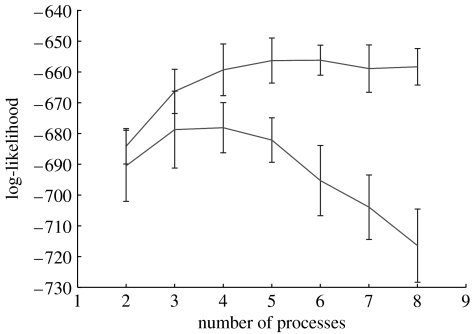
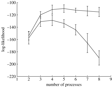
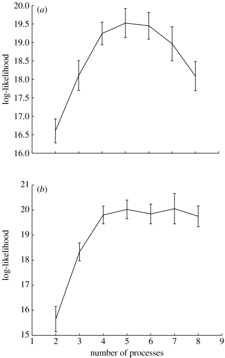
From the study of Sorlie et al. (2001) we used data from 115 primary breast carcinoma samples (labelled Norway/Stanford and very predominantly of invasive ductal type) and we used the same set of 534 genes selected in their study. In figure 1, we give the log-likelihood curves for both a maximum likelihood and maximum a posterior (MAP) model using variational LPD (Rogers et al. 2005). For the maximum likelihood model the log-likelihood has an approximate peak at about four processes indicating this is a suitable number of processes to use. For the MAP model (figure 1, upper curve) a Bayesian prior has been used to penalize construction of an over-complex model. The log-likelihood rises to a plateau after which no further gain is to be made by introducing further processes, since the model will not exploit this extra freedom. In contrast, for the maximum likelihood solution, the log-likelihood falls as further processes are introduced, since the algorithm will use these and construct an over-complex model.
Figure 1.
The log-likelihood (y-axis) versus number of processes (x-axis) using the MAP solution (upper curve) and maximum likelihood solution (lower curve) for the Sorlie et al. dataset Stanford/Norway dataset (Sorlie et al. 2001).
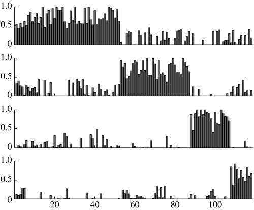
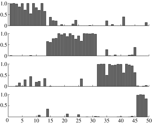
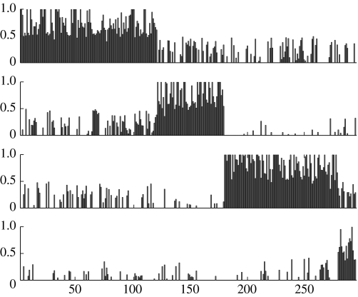
Using a four process model we can derive the decomposition diagram in figure 2, where the peaks represent the confidence that sample a is assigned to process k (these peaks are given by normalized γak parameters, see appendix B, equation (B 4) for further details). Unlike most cluster analysis methods, samples can belong to several processes simultaneously.
Figure 2.
Decomposition diagram derived from LPD for the dataset of Sorlie et al. (2001). The top process is identified with the trend curve 3 in figure 3a, the second process is identified with 2, the third with 4 and the lowest is identified with the indolent process 1 in figure 3a.
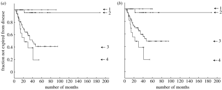
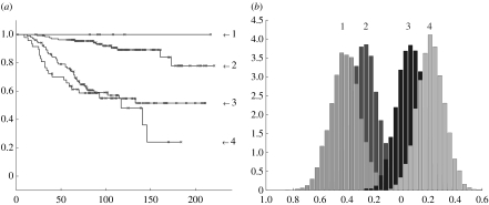
We have used a threshold of 0.5 for assignment of sample a to process k and determined the corresponding Kaplan–Meier plot in figure 3a. The separation is more distinct than that made by the original authors (Sorlie et al. 2003) with one indolent subtype and three aggressive subtypes indicated.
Figure 3.
Kaplan–Meier plots for the Sorlie et al. (2001) dataset. The graphs show fraction not expired from the disease (y-axis) versus number of months (x-axis). (a) For KM1 there are nine patients in process 1, 32 in 2, 48 in 3 and 18 in 4 (the remaining eight samples are insufficiently identified with a process). A vertical drop indicates expiry from the disease and a star indicates the patient is not recorded as expired from the disease (this includes the point at which some patients exited the survey). (b) KM2 corresponds to a different initialization of the algorithm (see text) with 7, 23, 58 and 18 patients assigned to processes 1 to 4, respectively. With different initializations there is some variability in the assignment of patients to processes 1 to 3, though process 4 remains quite distinct with 18 patients usually assigned, both using the variational LPD used here and the alternative MCMC approach described in appendix B (see figure 18a).
The likelihood function is not concave (local maxima can exist). Local maxima correspond to models with good fits to the data with the intervening regions in model space corresponding to poorer fits. Nevertheless, it is likely that models with good fits are sharply concentrated in model space. However, this does mean different initializations of the algorithm can give different solutions. In fact, since many peaks in figure 2 are near 0.5, the Kaplan–Meier plot is the most sensitive result dependent on this effect. Figure 3b is a typical result from a different initialization in which some patients have moved between the outcome trends. To investigate this issue we restarted the algorithm with 50 randomly constructed initializations and found that 32 of these gave a Kaplan–Meier plot in which no patient had expired from the disease in process 1. Furthermore, these 32 solutions had a distinctly higher average log-likelihood than those solutions with at least one patient expiring from the disease in process 1, indicating they are more appropriate models (figure 4).
Figure 4.
With 50 random initializations, 32 instances gave Kaplan–Meier plots with a purely indolent process 1 (lower histogram) and 18 cases had at least one patient expiring from the disease (upper histogram). The x-axis gives the value of the log-likelihood and the y-axis the frequency of occurrence. Solutions with a purely indolent process 1 gave a higher average log-likelihood indicating they give a better fit to the data.
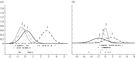
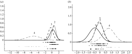
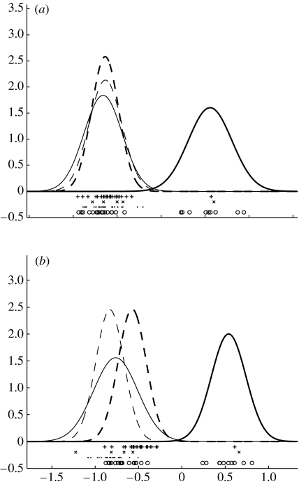
Apart from identifying samples with processes, LPD can be used to identify those genes which are most prominent in distinguishing processes. From the algorithm (equations (B 5), (B 6), (B 11) and (B 12) in appendix B), we can determine a mean μk and standard deviation σk for each process k and hence inferred density curves (estimating amount of data in a region). An example of two density curves is given in figure 5a,b. These density curves are derived from the dataset taken as a whole and are not one-dimensional fits to the expression values for that gene. We can thus use a score to rank genes distinguishing processes 1 and 2, for example, and this score follows a normal probability distribution with (0,1). Apart from comparing two processes we could also compare one process with the rest, e.g. by using the lowest pairwise Z1-score. Unfortunately, this score can be adversely influenced by large variances. Thus, the gene depicted in figure 7a does not score well because it has a large variance in the denominator of Z1. Consequently, we will also use a second, rank-based, score (based on the Mann–Whitney test; Rees 2001) to highlight such cases. This score will be denoted Z2 and quantifies the probability of observing a sequence of ranked and labelled datapoints (ranked by expression level and labelled 1 (process of interest) or 2 (other processes)).
Figure 5.
Inferred densities for (a) GRB7 and (b) ERBB2 for the Sorlie et al. (2001) dataset, with + the expression values for samples identified with process 3. Though only over-expressing in process 3 a subset of samples do not over-express GRB7 suggesting a possible subprocess within this process. In this and subsequent figures individual expression values are marked ○ if the samples are associated with process 1, × with 2, + with 3 and · if associated with process 4.
Figure 7.
(a) FOXA1 (HNF3A) underexpresses while (b) FOXC1 overexpresses in process 4 (· denotes the expression values in process 4).
No single gene is a particularly distinct marker for process 1. However, of the top 20 ranked genes distinguishing process 1 from the rest, all but one exhibit relative under-expression in process 1. For the three aggressive processes (2–4), process 4 has the most distinctive genes and process 2 the least distinctive (the highest ranked gene is LIV-1). Using the Z1-score the most distinctive gene in process 3 is GRB7, depicted in figure 5a. It has a score Z1=3.84 (p=0.000 06) with only Z1=1.59 (p=0.06) for the next highest ranked gene (PAPSS2). GRB7 is an adaptor-type signalling protein which is recruited via its SH2 domain to a variety of receptor tyrosine kinases, including ERBB2 and ERBB3. It is overexpressed in breast, oesophageal and gastric cancers, and may contribute to invasiveness potential (Pero et al. 2003). It is frequently co-amplified with ERBB2 (HER2) in breast cancer and from figure 5b we see that ERBB2 is, indeed, only overexpressed in process 3.
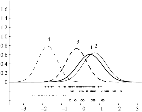
Process 4 has the most distinctive set of genes. In agreement with previous observations (Sorlie et al. 2003), this process has basal cell characteristics, e.g. cytokeratin 5 appears up-regulated. Using the Z1 score the top ranked gene distinguishing process 4 is FLT1 (VEGFR1; figure 6). VEGFR1 (especially its soluble isoform) is a negative regulator of vascular endothelial growth factor availability. Indeed, VEGFR1 overexpression is associated with improved survival in breast cancer (Zhukova et al. 2003). Oestrogen mediated decrease in VEGFR1 expression can cause increased angiogenesis leading to enhanced breast tumour progression (Elkin et al. 2004).
Figure 6.
Inferred densities for FLT1 (VEGFR1) in process 4 with · denoting the corresponding expression values.
The second ranked gene by Z1-score is MAFG which is associated with up-regulation of protective anti-oxidant enzymes under cellular conditions of oxidative stress (Katsuoka et al. 2005). Third ranked is FOXC1, a gene which expresses a forkhead transcription factor. The fourth ranked gene is XBP1 expressing an X box binding protein and the fifth ranked gene expresses AD021 protein. In table 1 we list the top 12 probes ranked by the Z2 score for process 4.
Table 1.
The top ranked genes distinguishing process 4 by Z2-score for the dataset of Sorlie et al. (Z2 follows a normal distribution with (0,1) thus the associated probabilities of occurrence are upper bounded by 10−8 reflecting the fact that the ordering of expression values for process 4 against the set of expression values for the other processes is highly improbable according to a null hypothesis. In the original data the FOXC1 clone is annotated as FLJ11796 and FOXA1 as HNF3A.)
| rank | gene | Z2-score | expression |
|---|---|---|---|
| 1 | TFF3 | 6.35 | under |
| 2 | FOXC1 | 6.32 | over |
| 3 | FOXA1 | 6.30 | under |
| 4 | XBP1 | 6.25 | under |
| 5 | GATA3 | 6.11 | under |
| 6 | B3GNT5 | 6.08 | over |
| 7 | FLJ14525 | 6.05 | over |
| 8 | FLT1 | 6.04 | under |
| 9 | GALNT10 | 5.95 | under |
| 10 | FOXC1 | 5.88 | over |
| 11 | FBP1 | 5.76 | under |
| 12 | GATA3 | 5.68 | under |
FOXA1 and FOXC1 are members of the forkhead family of transcription factor genes (figure 7).
FOXA1, GATA3 and XBP1 encode transcription factors and their roles and association with the oestrogen receptor-α gene (ESR1) and trefoil factors (TFF3 and TFF1) are reviewed by Lacroix & Leclerq (2004).
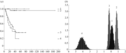
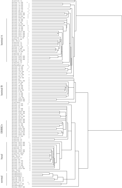
In appendix A we give the original dendrogram decomposition reported in Sorlie et al. (2003) along with the assignment to processes given in figure 2. Sorlie et al. (2003) labelled a subset of the tumour samples as luminal A and B, ERBB2+ and Basal. Their 18 Basal tumours match the 18 process 4 samples. Indeed, we shall later see that this process is very distinctive. Elsewhere LPD labels a wider range of samples than labelled by Sorlie et al. (though this would depend on the threshold chosen for the significance of the peaks in figure 2). Their 11 luminal B and 11 ERBB2+ are exclusively subsets of process 3, while their 28 luminal A are exclusively associated with processes 1 and 2. Indolent process 1 is exclusively sampled from some luminal A samples and other samples which were left unlabelled in their study. If we use the MCMC-based approach to LPD we obtain a very similar picture (see figure 18).
Figure 18.
(a) Kaplan–Meier plot and (b) distribution of means for FOXA1 from the MCMC algorithm applied to the Sorlie et al. (2001) dataset. For the Kaplan–Meier plot there are 11 patients in process 1, 30 in process 2, 42 in process 3 and 18 in process 4. (b) Distribution of means for a selected gene (FOXA1) indicating the reliability of the point estimates of the means found using LPD (see figure 7a for comparison).
2.2 West et al. dataset
For the Affymetrix breast cancer dataset of West et al. (2001) we used data from 49 samples (exclusively derived from tumours of invasive ductal type) with 500 probes ordered using the p-values derived by the authors (though LPD can readily handle the full dataset, some feature selection is advisable, since redundant information injects noise into the analysis). No survival data were available for this dataset, though time-to-metastasis was available. Nevertheless, we can derive the corresponding MAP solution (figure 8).
Figure 8.
The log-likelihood (y-axis) versus number of processes (x-axis) using a MAP approach (right) for the West et al. (2001) dataset.
The onset of the plateau is more ambiguous in this case and could indicate up to five processes. However, to conform with the analysis elsewhere we will use 4. We then get the decomposition diagram as in figure 9.
Figure 9.
Decomposition diagram derived from LPD for the dataset of West et al. (2001).
As observed previously, process 4 has the most distinctive genetic signature which, from time-to-metastasis data, appears identified with the second row in figure 9. The top-ranked genes distinguishing this process are given in table 2.
Table 2.
Top ranked genes using the Z2-score distinguishing a tentative process 4. (Using the Z1 score GATA3 is ranked second, FOXA1 is third, XPB1 is fourth and TFF3 is sixth. The probabilities of occurrence are upper bounded by 2×10⁻⁶ (for Z2=4.78).)
| rank | gene | Z2-score | expression |
|---|---|---|---|
| 1 | hCRHP | 5.51 | under |
| 2 | XBP1 | 5.50 | under |
| 3 | FOXA1 | 5.26 | under |
| 4 | FPB1 | 4.98 | under |
| 5 | FLJ13710 | 4.94 | under |
| 6 | GATA3 | 4.94 | under |
| 7 | GATA3 | 4.92 | under |
| 8 | CNAP1 | 4.90 | over |
| 9 | NFIB2 | 4.83 | over |
| 10 | human complement factor B | 4.83 | under |
| 11 | TFF3 | 4.79 | under |
| 12 | FLJ13710 | 4.78 | under |
Interestingly, GATA3, FOXA1, XPB1, TFF3 and FPB1 are in common between tables 1 and 2. Though GRB7 and ERBB2 were highlighted previously (Sorlie et al. 2003) the associated p-values and sample sizes indicate they do not have a statistically significant elevated expression here, though this fact most likely stems from the smaller dataset size.
2.3 van 't Veer et al. dataset
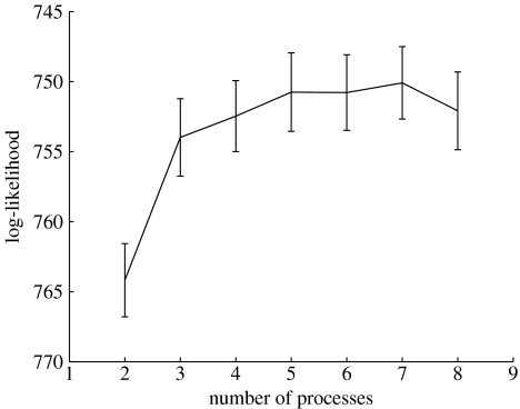
For the dataset of van 't Veer et al. (2002), we used samples from 78 patients with primary breast carcinomas, a further 18 samples from patients with BRCA1 germline mutations and 2 samples with BRCA2 mutations. We used 500 genes selected using the p-values derived by the authors (van 't Veer et al. 2002), using those genes with a p-value of less than 0.01 in more than 30 tumours. Survival data are not available though we can still compute the log-likelihood curves (figure 10) and this suggests a peak at four processes.
Figure 10.
The log-likelihood (y-axis) versus number of processes (x-axis) using the MAP solution (upper, plateauing curve) and maximum likelihood (lower curve) solution for the Van 't Veer et al. (2002) dataset.
The spectrum of peaks corresponding to figure 2 indicated that 16 of the 18 BRCA1 mutation carriers belonged in one process (which, from the time to metastasis data, appeared to be process 4 in figure 3). The other 2 BRCA1 samples were spread between processes and, interestingly, were the only two patients not to proceed to metastasis. The two BRCA2 samples belonged together in the same process, distinct from the process associated with the BRCA1 samples. This picture agreed with the interpretation by dendrogram of Sorlie et al. (2003).
Using the Z1-score, one process has ERRB2 (figure 11a) and GRB7 (figure 11b) in second and third ranked position with the distribution of expression values having a similar bimodal distribution to that in figure 5a,b.
Figure 11.
Inferred densities for (a) GRB7 and (b) ERBB2 for the dataset of van 't Veer et al. (2002).
The highest ranked Z2-scores for genes in the four processes are 7.02, 5.85, 5.61 and 2.87. Interestingly, the most distinctive process (with Z2=7.02) is associated with genes described previously for process 4, such as TFF3 and FOXC1 (table 3). TFF3, and the GATA3, FOXA1 and XPB1 genes mentioned previously, all feature in a small gene expression graph derived from a sparse graphical model (Dobra & West 2004; Dobra et al. 2004) indicating genes closely linked with the oestrogen receptor gene.
Table 3.
TFF3 and FOXC1 are first and third ranked for the most distinctive process in the dataset of van 't Veer et al. (2002). (Similarly they are first and second ranked for the most distinctive and aggressive process (4) in the data of Sorlie et al. (table 1).)
| rank | gene | Z2-score | expression |
|---|---|---|---|
| 1 | TFF3 | 7.02 | under |
| 2 | AGR2 | 6.89 | under |
| 3 | FOXC1 | 6.79 | over |
| 4 | GABA | 6.75 | over |
| 5 | VGLL1 | 6.68 | over |
2.4 de Vijver et al. dataset
The study of van 't veer et al. preceded a larger study by de Vijver et al. (2002) which used 295 samples from patients with primary breast carcinomas. The authors of this study discovered tentative signatures for poor and good prognosis using a reduced 70 gene set selected from 24 479. In figure 14, we present a Kaplan–Meier plot with the lower dashed curve corresponding to patients in the poor signature cohort and the upper dashed curve corresponding to the good signature cohort. In figure 12a we have re-analysed the same dataset (295 samples, 70 features) using variational LPD and a maximum likelihood approach. The curve shows a peak in the range 4–6 processes, implying that the 2-process model proposed by the original authors (de Vijver et al. 2002) is a sub-optimal interpretation of the data. In figure 12b, we see that the likelihood curve for the MAP solution plateaus after using four processes.
Figure 14.
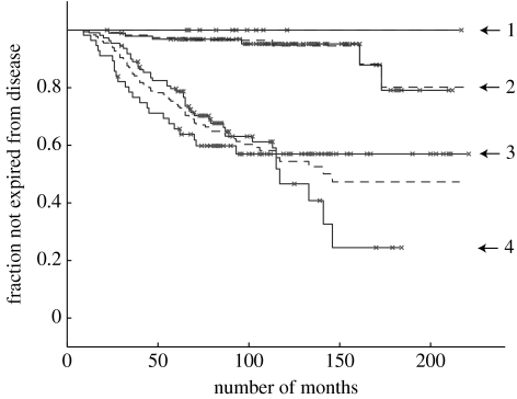
Kaplan–Meier plot for the processes identified in figure 13: fraction not expired from the disease (y-axis), versus number of months (x-axis). The curves labelled 3 and 4 meet at the midpoint but do not cross over. The number of patients identified with each curve is 12 (process 1), 97 (2), 110 (3) and 56 (4; these numbers do not sum to 295 because some samples are ambiguously identified). The original split of de Vijver et al. (2002) are given as dashed curves for comparison.
Figure 12.
The log-likelihood (y-axis) versus number of processes (x-axis) using a (a) maximum likelihood and (b) MAP approach for the de Vijver et al. (2002) dataset.
If we plot the corresponding Kaplan–Meier curves for figure 13 we get the curves in figure 14 in which the top process in figure 13 is identified with curve 3 in figure 14, the second process is identified with curve 4, the third process with 2 and the fourth (lowest) with 1. Compared to the original analysis of de Vijver et al. (dashed curves in figure 14), all patients in processes 3 and 4 derive from their lower (poor prognosis) group while 10 patients in process 1 are derived from their upper (good prognosis) group and 2 are derived from their poor prognosis group. All patients in process 2 derive from their good prognosis group. Thus, our analysis is compatible with their description while enhancing the distinction between clinical outcomes (the solution presented here corresponds to the highest likelihood solution found in numerical experiments). With the MCMC-based algorithm we obtain a very similar Kaplan–Meier plot (figure 19).
Figure 13.
A 4 process decomposition of the dataset of de Vijver et al. (2002) using variational LPD.
Figure 19.
(a) Kaplan–Meier plot using the MCMC approach for the de Vijver et al. (2002) dataset. For the Kaplan–Meier plot there are six patients in process 1, 136 in process 2, 103 in process 3 and 47 in process 4. The curves labelled 3 and 4 meet but do not cross. (b) Distribution of means for ORC6L giving a similar progression to that observed in figure 15a.
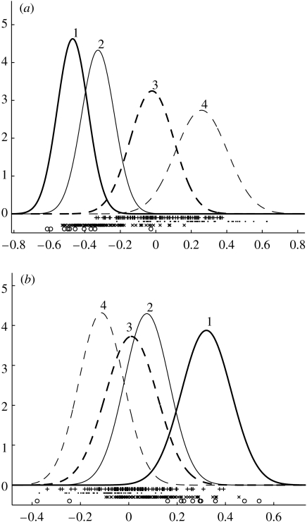
The inferred densities for two top-ranked genes separating processes 1 and 4 are given in figure 15a,b. In fact, of the 26 top-ranked genes separating processes 1 and 4, 21 genes move from under-expression to over-expression as we progress from indolent to the most aggressive subtype, following the trend in figure 15a, while four genes follow the reverse trend illustrated in figure 15b.
Figure 15.
Inferred densities for (a) ORC6L and (b) STK32B. The individual expression values are given below the inferred density curves, with ○ associated with process 1, × with 2, + with 3 and · with process 4.
The observation that most of the listed genes under-express in process 1 agrees with an observation for the dataset of Sorlie et al. in which we found that 19 from the top ranked 20 genes distinguishing process 1 from the others under-expressed on the average in process 1. The gene names, their mean expression values per process and this trend are discussed in further detail in appendix C to this paper.
3. Conclusion
The results are broadly consistent and indicate at least four principal processes for primary breast carcinoma. Our analysis suggests the existence of an indolent subtype distinguished by under-expression across a number of genes associated with tumour growth. Since, some patients in this process do develop metastatic tumours this process is not wholly benign, nor does it consist of misidentified normal samples. There is a subtype closely related to the luminal A subtype proposed by Sorlie et al. (2003). In line with previous observations there is also a subtype marked by up-regulation of ERBB2 (HER2) and GRB7. As noted in figures 5 and 11 there is an apparent bimodal distribution and ERBB2 and GRB7 do not uniformly over express in this process. Given the split observed in the dendrogram (appendix A) this may indicate two subprocesses, one with elevated expression levels for these genes. However, we did not find a statistically significant difference in clinical outcome for patients belonging to these two possible subclasses. The most aggressive subtype is also the most well defined: it is clearly and consistently identified by both variants of LPD (figures 3 and 18a) and matches the basal subtype described by Sorlie et al. (figure 16). This subtype is marked by abnormal expression of the transcription factor genes FOXA1, FOXC1, GATA3, TFF3 and XBP1, for example, and it is associated with loss of regulation of the vascular growth factor VEGF. As already remarked, using a sparse graphical model (Dobra & West 2004; Dobra et al. 2004), we find that the transcription factor genes FOXA1, GATA3, TFF3 and XBP1 are closely linked with the oestrogen receptor-alpha gene, which with the oestrogen pathway, plays a crucial role in the development of many breast tumours. One target of ERα is the TFF1 gene and FOXA1 has a direct influence on transcription by this gene, since there are binding sites for FOXA1 in its promoter region (Beck et al. 1999). A number of other ERα-bound promoters have FOXA1 binding sites (Laganiere et al. 2005). The role of FOXA1 has been highlighted in a contemporary study by Laganiere et al. (2005): expression by FOXA1 correlates with the presence of ERα and it has been suggested that that this gene plays a crucial role in a transcriptional domain governing oestrogen response. Reinforcing this result, a contemporary study by Carroll et al. (2005) has shown that forkhead factor binding sites are present in 54% of 57 ER binding regions. This strongly supports the significance of abnormal expression of FOXA1 and FOXC1 indicated by our analysis. Finally, in agreement with the analysis using a sparse graphical model (Dobra & West 2004; Dobra et al. 2004), there appears to be an important role played by TFF3, a close relative of TFF1.
Figure 16.
A comparison between the dendrogram reported in Sorlie et al. (2003), Fig. 1b, and the decomposition by variational LPD given in figure 2.
The decomposition proposed here is at most a basic model, since one would expect further subdivision as more data becomes available, thus enabling a higher resolution picture. As remarked previously, the effects of noise are averaged out as the dataset size increases. Thus, for the dataset of Sorlie et al. the peak in the likelihood curve is at 3–4 processes but, for the largest dataset of de Vijver et al. it is approximately 4–5. Certainly, our analysis suggests that the 2 process split of de Vijver et al. (2002) is too simple a model and at least four main processes are justified by the datasets used. The dataset for West et al. was exclusively based on invasive ductal tumours and the Sorlie et al. dataset had samples very predominantly of this type. However, use of samples consistently of the same histological type would also help reduce noise and improve definition. The indolent subtype 1 was not presented in the original analysis of Sorlie et al. and the ability of the method to find this feature highlights the importance of using Bayesian methods in this context.
Appendix A. Comparison with dendrogram of Sorlie et al.
Figure 16 gives a comparison between the dendrogram reported in Sorlie et al. (2003), Fig. 1b, and the decomposition by variational LPD given in figure 2. To the left of the tree, the variational LPD assignment to process is designated by the numbers 1–4. Beside these numbers are the sample titles for identification with Sorlie et al. (2003), figure 1b. Process assignment numbers are missing in a few cases because the peak in figure 2 (normalized γak, see equation (B 4), appendix B) is ambiguous in its assignment of sample to process.
Appendix B. Latent process decomposition
B.1 Variational approach to LPD
We will briefly outline latent process decomposition (for a more detailed description of the method the reader is referred to Rogers et al. (2005)). As remarked in the text, a sample can be represented as a combinatorial mixture over multiple processes, in contrast to the implicit mutual exclusion of classes assumption of most cluster analysis methods. Thus, we have used process rather than cluster to emphasis this difference with standard cluster analysis methods.
We are interested in constructing a model for the microarray data and this model will have parameters which we alter during the training process. We will suppose these parameters are r1, r2, … or, as a set, . Similarly the dataset will be denoted by . Thus, we wish to maximize the probability of a model given the data, p(|), which from Bayes's rule can also be written as
| (B1) |
where p(|) is the likelihood and p() is the prior on our parameters .
The approach we now outline is described in more detail elsewhere (Rogers et al. 2005) and it adopts the LDA approach to data modelling (Blei et al. 2003), comparing favourably with alternatives such as mixture models (McLachlan et al. 2002), Naive Bayes and other approaches (see Rogers et al. 2005). In this approach, we incorporate prior beliefs in the form of reasonable distributional assumptions, e.g. the (logged) gene expression levels from a microarray experiment are assumed approximately normally distributed (for Affymetrix data we use a prior affine translation to bring expression data into an approximate (0,1) distribution). Unfortunately, we cannot estimate the above posterior probability directly but we can lower bound this expression using Jensen's inequality. Thus, our approach parallels the LDA method of Blei et al. (2003) which derives a similar lower bound for discrete data. This lower bound is found using an efficient algorithmic technique, described below.
We are interested in finding the set of parameters that maximizes p(|). In the case of a uniform (or uninformative) prior, this is the maximum likelihood solution. We will begin by deriving the maximum likelihood solution and then extend the method to a non-uniform prior. The log-likelihood of a set of training samples is , where μ, σ, α are the model parameters, the process means, standard deviations and Dirichlet parameter, respectively. Marginalizing over the latent variable θ allows us to expand this expression as follows
| (B 2) |
A lower bound on this expression can be inferred by the introduction of two variational parameters Qkga and γak and the following iterative update equations provide estimates for these parameters
| (B3) |
| (B 4) |
for given αk, with process index k=1, …, , and where (…) is a normal distribution and ψ(z) is the digamma function. For gene g and process k, μgk and σgk are the means and standard deviations (for example, in figure 5 these give the means and spreads for the four processes illustrated). γak, normalized over the number of processes, gives the confidence of membership of sample a in process k. Let ega denote the expression level for gene g in sample a, then the model parameters are obtained from the following update equations
| (B 5), (B 6), (B 11) |
| (B6) |
The update rule for the Dirichlet model parameter αk is found from the derivatives of the α dependent terms in the likelihood (Blei et al. 2003). Thus, the αk are modified after each iteration of the above updatings using a standard Newton–Raphson technique (see Blei et al. 2003, Appendix A.4.2; Rogers et al. 2005).
The above argument can be extended to a MAP solution with non-uniform priors. Thus, a suitable prior on the means could be a Gaussian distribution with zero mean. This would reflect a prior belief that for cDNA microarrays most genes will be uninformative and will have logged expression ratios around zero (i.e. they are unchanged compared to a reference sample). For the variance, we may wish to define a prior that penalizes over-complex models and avoids overfitting. Overfitting may occur when Gaussian functions contract onto a single data point causing poor generalization. With a suitable choice for the prior an extension of our model to a full MAP solution is straightforward. Our combined likelihood and prior expression is (assuming a uniform prior on α)
| (B7) |
Taking the logarithm of both sides we see that the maximization task is given by
| (B8) |
Thus, we can simply append these terms onto our bound on the log-likelihood. Noting that they are functions of μ and σ only (and any associated hyper-parameters), we conclude that these extra terms only change the update equations for μak and σak. Let us assume the following priors:
| (B 9) |
| (B 10) |
then we obtain the following new update equations instead
| (B11) |
| (B 12) |
Once the model parameters have been estimated, we can calculate the likelihood for a collection of ′ samples using
| (B13) |
where we estimate the expectation over the Dirichlet distribution by averaging over N samples drawn from the estimated Dirichlet prior p(θ|α)
| (B14) |
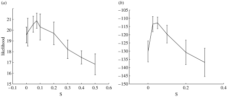
Apart from using the likelihood to determine the best number of processes to use, it can be used to determine the parameters used in the prior. In figure 17 we plot likelihood curves as a function of s, the prior parameter in equation (B 10). The peaks in these plots model the extent of noise in the data and enables the algorithm to avoid constructing an over-complex model which would fit to this noise. As reported elsewhere (Rogers et al. 2005) the model is little affected by choice of the prior parameter σμ in equation (B 9) and we have set this value to 0.1.
Figure 17.
Hold-out log-likelihood as a function of s for the datasets of (a) Sorlie et al. (2001) and (b) van 't Veer et al. (2002).
B.2 Markov Chain Monte Carlo approach to LPD
To validate the above variational method we re-derived the results using a Gibbs sampler-based approach for the datasets of Sorlie et al. and de Vijver et al. The starting point, equation (B 2), is the same but otherwise the method is distinct. The approach we now describe is slow to execute (the cross-validation study of the number of processes proved prohibitive). However, it supports the results presented in the main text. Also, by using a Gibbs sampler we can obtain a full posterior distribution for the model parameters and hence investigate the accuracy of the point estimate approximations derived by the variational algorithm described above.
We implemented a standard Gibbs sampler (Mackay 2003) using conjugate priors for all model parameters. Each variable in the algorithm was initialized randomly. We used a burn-in period to allow the Monte Carlo algorithm to stabilize (100 000 iterations for the Sorlie et al. dataset and 40 000 for de Vijver et al.). The next 10 000 samplings were used to form the posterior distribution. To compare with variational LPD we chose four processes. For process membership there is no γ parameter so instead we determined membership from the normalized mode of the posterior distribution of θ. For the Sorlie et al. dataset we give the resulting Kaplan–Meier plot in figure 18a, which can be compared to figure 3a from the variational approach. The posterior distribution over model parameters supported the significance of genes already discussed. For example, in figure 18b we give the distribution over means for FOXA1 which can be compared to figure 7a with point estimates of the means from the variational approach.
For the dataset of de Vijver et al. and using the MCMC approach, we give the Kaplan–Meier plot in figure 19a. As for the variational approach we find one indolent process and further processes of increasing aggressiveness. For comparison with figure 15a we give the distribution of means for ORC6L in figure 19b.
Appendix C. Supplementary material on the dataset of De Vijver et al.
In the original publication of de Vijver et al. (2002) 21 cDNA sequences had no gene name or information associated with them. Given this fact and the monotonic trends in mean expression values mentioned in the main text we have updated and examined ontology information for the 70 genes and their encoded proteins to examine their significance. A full description of all 70 entries and further information is available as supplementary data at www.enm.bris.ac.uk/lpd/bc.htm. In table 4 we list the top ranked genes distinguishing process 1 versus process 4 (with Z1>2) for the dataset of de Vijver et al. The four columns headed process are the mean logged expression values (using log base 10). The processes are ranked in order of most indolent (1) to most aggressive (4) outcome. The end column highlights the progression trend across the four processes. Genes marked BCSS1 and BCSS2 correspond to hypothetical genes: BCSS1 is ‘moderately similar to T50635 hypothetical protein’ and BCSS2 is ‘weakly similar to ISHUSS disulfide-isomerase’. The Z1 values follow a normal probability distribution (0,1).
Table 4.
Gene names, mean expression values and expression trends for the top-ranked 26 genes distinguishing process 1 from process 4.
| gene ID | gene name | process 1 | process 2 | process 3 | process 4 | Z1 | trend |
|---|---|---|---|---|---|---|---|
| NM_014321 | ORC6L | −0.47 | −0.32 | −0.02 | 0.26 | 4.29 | up |
| Contig55725_RC | BCSS1 | −0.80 | −0.54 | −0.22 | 0.39 | 4.15 | up |
| NM_018401 | STK32B | 0.32 | 0.07 | 0.01 | −0.11 | 3.14 | down |
| AB037863 | KIAA1442 | 0.28 | 0.05 | −0.01 | −0.29 | 3.07 | down |
| Contig38288_RC | BCSS2 | −0.34 | −0.16 | −0.02 | 0.26 | 3.06 | up |
| NM_003981 | PRC1 | −0.45 | −0.30 | 0.02 | 0.24 | 2.98 | up |
| NM_016359 | NUSAP1 | −0.50 | −0.28 | 0.039 | 0.22 | 2.93 | up |
| NM_004702 | CCNE2 | −0.55 | −0.32 | −0.02 | 0.22 | 2.93 | up |
| NM_001809 | CENPA | −0.52 | −0.41 | −0.06 | 0.29 | 2.80 | up |
| AL137718 | DIAPH3 | −0.30 | −0.10 | 0.03 | 0.22 | 2.78 | up |
| NM_014791 | MELK | −0.46 | −0.21 | 0.01 | 0.26 | 2.71 | up |
| NM_016448 | RAMP | −0.36 | −0.17 | 0.05 | 0.15 | 2.65 | up |
| Contig40831_RC | AI224578 | −0.39 | −0.11 | −0.05 | 0.19 | 2.57 | up |
| AL080059 | TSPYL5 | −0.53 | −0.24 | −0.15 | 0.25 | 2.50 | up |
| Contig46218_RC | DIAPH3 | −0.35 | −0.22 | 0.04 | 0.27 | 2.50 | up |
| NM_003875 | GMPS | −0.34 | −0.17 | −0.05 | 0.21 | 2.45 | up |
| NM_020974 | SCUBE2 | 0.24 | 0.19 | −0.24 | −0.99 | 2.39 | down |
| NM_000436 | OXCT1 | −0.29 | −0.06 | −0.10 | 0.15 | 2.37 | mixed |
| NM_005915 | MCM6 | −0.37 | −0.14 | 0.00 | 0.23 | 2.31 | up |
| AA555029_RC | AA555029 | −0.31 | −0.09 | −0.06 | 0.15 | 2.27 | up |
| NM_002916 | RFC4 | −0.29 | −0.133 | −0.01 | 0.20 | 2.27 | up |
| AL080079 | GPR126 | −0.59 | −0.25 | −0.12 | 0.17 | 2.22 | up |
| NM_015984 | UCHL5 | −0.21 | −0.08 | −0.01 | 0.15 | 2.13 | up |
| Contig20217_RC | TGS | −0.33 | −0.17 | −0.02 | 0.17 | 2.08 | up |
| NM_006117 | PECI | 0.21 | 0.05 | 0.01 | −0.25 | 2.07 | down |
| Contig32185_RC | ITS | −0.33 | −0.14 | −0.08 | 0.15 | 2.02 | up |
Of these genes, ORC6L is involved in DNA replication and serves as a platform for the assembly of additional initiation factors such as CDC6 and MCM. siRNA gene silencing studies indicate that ORC6L plays an essential role in coordinating chromosome replication and segregation with cytokinesis. STK32B is a serine/threonine kinase. KIAA1442 encodes a transcription factor with an IPT/TIG motif. These motifs are found in cell surface receptors such as Met and Ron as well as in intracellular transcription factors, where it is involved in DNA binding. Intriguingly the Ron tyrosine kinase receptor shares with the members of its subfamily (Met and Sea) the control of cell dissociation, motility, and invasion of extracellular matrices (scattering; Collesi et al. 1996). Two genes have no known function though Contig38288RC is weakly similar to ISHUSS protein disulfide-isomerase, an enzyme that participates in the folding of proteins containing disulfide bonds. In table 4 we have labelled Contig55725RC as BCSS1 and Contig38288RC as BCSS2 (breast cancer survival signature 1 and 2). Many genes are involved in processes associated with tumour growth such as DNA replication (MCM6), cell cycle control (CCNE2), spindle associated factors (NUSAP1, PRC1), chromosome organization (CENPA), actin filament assembly (DIAPH3) and vascular remodelling (ITS). All these genes are up-regulated for the most aggressive process versus the least aggressive. DIAPH3, which was unidentified in the original paper, appears three times in the 70 gene set.
References
- Beck S, Sommer P, Do Santos Silva E, Blin N, Gott P. Hepatocyte nuclear factor 3 (winged helix domain) activates trefoil factor gene TFF1 through a binding motif adjacent to the TATA box. Cell Biol. 1999;18:157–164. doi: 10.1089/104454999315547. [DOI] [PubMed] [Google Scholar]
- Ben-Tovin Jones L, Ng S, Ambroise C, Monico K, Khan N, McLachlan G.J. Use of microarray data via model-based classification in the study and prediction of survival from lung cancer. In: Shoemaker J.S, Lin S.M, editors. Methods of microarray data analysis IV. Springer; New York: 2005. pp. 163–173. [Google Scholar]
- Blei D, Ng A, Jordan M. Latent Dirichlet allocation. J. Mach. Learn. Res. 2003;3:993–1022. [Google Scholar]
- Brunet J, Tamayo P, Golub T, Mesirov J. Metagenes and molecular pattern discovery using matrix factorization. Proc. Natl Acad. Sci. USA. 2004;101:4164–4169. doi: 10.1073/pnas.0308531101. doi:10.1073/pnas.0308531101 [DOI] [PMC free article] [PubMed] [Google Scholar]
- Carroll J, et al. Chromosome-wide mapping of estrogen receptor binding reveals long-range regulation requiring the forkhead protein FOXA1. Cell. 2005;122:33–43. doi: 10.1016/j.cell.2005.05.008. doi:10.1016/j.cell.2005.05.008 [DOI] [PubMed] [Google Scholar]
- Collesi C, Santoro M, Gaudino G, Comoglio P. A splicing variant of the RON transcript induces constitutive tyrosine kinase activity and an invasive phenotype. Mol. Cell. Biol. 1996;16:5518–5526. doi: 10.1128/mcb.16.10.5518. [DOI] [PMC free article] [PubMed] [Google Scholar]
- de Vijver M, et al. A gene expression signature as a predictor of survival in breast cencer. N. Engl. J. Med. 2002;347:1999–2009. doi: 10.1056/NEJMoa021967. doi:10.1056/NEJMoa021967 [DOI] [PubMed] [Google Scholar]
- Dobra, A. & West, M. 2004 Graphical model-based gene clustering and metagene expression analysis. Technical report.
- Dobra A, Jones B, Hans C, Nevins J, West M. Sparse graphical models for exploring gene expression data. J. Multivariate Anal. 2004;90:196–212. doi:10.1016/j.jmva.2004.02.009 [Google Scholar]
- Elkin M, Orgel A, Kleinman H. An angiogenic switch in breast cancer involves estrogen and soluble vascular endothelial growth factor receptor 1. J. Natl Cancer Inst. 2004;96:875–978. doi: 10.1093/jnci/djh140. [DOI] [PubMed] [Google Scholar]
- Flaherty P, Giaever G, Kumm J, Jordan M.I, Arkin A.P. A latent variable model for chemogenomic profiling. Bioinformatics. 2005;21:3286–3293. doi: 10.1093/bioinformatics/bti515. doi:10.1093/bioinformatics/bti515 [DOI] [PubMed] [Google Scholar]
- Gruvberger S, et al. Estrogen receptor status in breast cancer is associated with remarkably distinct gene expression patterns. Cancer Res. 2001;61:5979–5984. [PubMed] [Google Scholar]
- Hedenfalk I, et al. Gene-expression profiles in hereditory breast cancer. N. Engl. J. Med. 2001;344:539–548. doi: 10.1056/NEJM200102223440801. doi:10.1056/NEJM200102223440801 [DOI] [PubMed] [Google Scholar]
- Katsuoka F, Motohashi H, Engel J, Yamamoto M. NRF2 transcriptionally activates the MAFG gene through an antioxidant response element. J. Biol. Chem. 2005;280:4483–4490. doi: 10.1074/jbc.M411451200. doi:10.1074/jbc.M411451200 [DOI] [PubMed] [Google Scholar]
- Lacroix M, Leclerq G. About GATA3, HNF3A and XBP1, three genes co-expressed with the oestrogen receptor-alpha gene (ESR1) in breast cancer. Mol. Cell. Endocrinol. 2004;219:1–7. doi: 10.1016/j.mce.2004.02.021. doi:10.1016/j.mce.2004.02.021 [DOI] [PubMed] [Google Scholar]
- Laganiere J, et al. Location analysis of estrogen receptor α target promoters reveals that FOXA1 defines a domain of the estrogen response. Proc. Natl Acad. Sci. USA. 2005;102:11 651–11 656. doi: 10.1073/pnas.0505575102. doi:10.1073/pnas.0505575102 [DOI] [PMC free article] [PubMed] [Google Scholar]
- Mackay D. Cambridge University Press; Cambridge: 2003. Information theory, inference and learning algorithms, ch. 4. [Google Scholar]
- McLachlan G, Bean R, Peel D. A mixture model-based approach to the clustering of microarray expression data. Bioinformatics. 2002;18:413–422. doi: 10.1093/bioinformatics/18.3.413. doi:10.1093/bioinformatics/18.3.413 [DOI] [PubMed] [Google Scholar]
- Moloshok T, Klevecz R, Grant J, Manion F, Speier W, Ochs M. Application of Bayesian decomposition for analysing microarray data. Bioinformatics. 2002;18:566–575. doi: 10.1093/bioinformatics/18.4.566. doi:10.1093/bioinformatics/18.4.566 [DOI] [PubMed] [Google Scholar]
- Pero S, Daly R, Krag D. GRB7-based molecular therapeutics in cancer. Expert Rev. Mol. Med. 2003;5:1–11. doi: 10.1017/S1462399403006227. doi:10.1017/S1462399403006227 [DOI] [PubMed] [Google Scholar]
- Perou C, et al. Molecular portraits of human breast tumours. Nature. 2000;406:747–752. doi: 10.1038/35021093. doi:10.1038/35021093 [DOI] [PubMed] [Google Scholar]
- Rees D. 4th edn, ch. 11. Chapman & Hall; London: 2001. Essential statistics. [Google Scholar]
- Rogers S, Girolami M, Campbell C, Breitling R. The latent process decomposition of cDNA microarray datasets. IEEE/ACM Trans. Comput. Biol. Bioinform. 2005;2:143–156. doi: 10.1109/TCBB.2005.29. doi:10.1109/TCBB.2005.29 [DOI] [PubMed] [Google Scholar]
- Sorlie T, et al. Gene expression patterns of breast carcinomas distinguish tumor subclasses with clinical implications. Proc. Natl Acad. Sci. USA. 2001;98:10 869–10 874. doi: 10.1073/pnas.191367098. doi:10.1073/pnas.191367098 [DOI] [PMC free article] [PubMed] [Google Scholar]
- Sorlie T, et al. Repeated observation of breast tumor subtypes in independent gene expression data sets. Proc. Natl Acad. Sci. USA. 2003;100:8418–8423. doi: 10.1073/pnas.0932692100. doi:10.1073/pnas.0932692100 [DOI] [PMC free article] [PubMed] [Google Scholar]
- van 't Veer L, et al. Gene expression profiling predicts clinical outcome of breast cancer. Nature. 2002;415:530–535. doi: 10.1038/415530a. doi:10.1038/415530a [DOI] [PubMed] [Google Scholar]
- West M, et al. Predicting the clinical status of human breast cancer using gene expression profiles. Proc. Natl Acad. Sci. USA. 2001;98:11 462–11 467. doi: 10.1073/pnas.201162998. doi:10.1073/pnas.201162998 [DOI] [PMC free article] [PubMed] [Google Scholar]
- Zhukova L, Zhukov N, Lichinitser M. Expression of FLT-1 and FLK-1 receptors for vascular endothelial growth factor on tumor cells as a new prognostic criterion for locally advanced breast cancer. Bull. Exp. Biol. Med. 2003;135:478–481. doi: 10.1023/a:1024975627843. doi:10.1023/A:1024975627843 [DOI] [PubMed] [Google Scholar]


