Identifying the Environmental Factors That Determine the Genetic Structure of Populations

Abstract

The study of population genetic structure is a fundamental problem in population biology because it helps us obtain a deeper understanding of the evolutionary process. One of the issues most assiduously studied in this context is the assessment of the relative importance of environmental factors (geographic distance, language, temperature, altitude, etc.) on the genetic structure of populations. The most widely used method to address this question is the multivariate Mantel test, a nonparametric method that calculates a correlation coefficient between a dependent matrix of pairwise population genetic distances and one or more independent matrices of environmental differences. Here we present a hierarchical Bayesian method that estimates F_ST values for each local population and relates them to environmental factors using a generalized linear model. The method is demonstrated by applying it to two data sets, a data set for a population of the argan tree and a human data set comprising 51 populations distributed worldwide. We also carry out a simulation study to investigate the performance of the method and find that it can correctly identify the factors that play a role in the structuring of genetic diversity under a wide range of scenarios.

ONE of the fundamental problems in population genetics is the study of the nature of genetic differentiation that is found in real populations and, if possible, to identify the factors that are responsible for the observed spatial structuring of genetic diversity. A clear understanding of these issues is of fundamental importance for a wide range of applications that include, among others, the inference of population histories, biodiversity conservation, and the identification of disease genes and/or disease-resistant genes in humans and economically important species. There are many methods that estimate different measures of genetic differentiation among populations (Excoffier 2001; Rousset 2001) but there is a paucity of methods that allow us to identify factors that influence genetic structuring. The most commonly used method, the multivariate Mantel test (Smouse et al. 1986), is based on the calculation of genetic and environmental distance measures between every pair of populations.

Genetic structuring of neutral markers is a consequence of the amount of genetic drift to which each local population has been subjected, due to its local effective size and/or due to its overall degree of geographic/ecologic isolation. Thus, it seems appropriate to base the estimation on parameters and variables that are specific to each local population. However, the study of population genetic structuring is traditionally done using global measures such as F_ST or G_ST, which ignore differences in the strength of genetic drift across populations. Over a decade ago, Balding and Nichols (1995) proposed the use of population-specific F_ST's in the context of a migration–drift equilibrium model. They considered biallelic markers and modeled allele frequencies using a beta distribution with expectation p and variance p(1 − p)/(1 + θ) so that F_ST = 1/(1 + θ). Such a formulation enabled them to use a likelihood-based approach to estimate population-specific F_ST's. More recently, Nicholson et al. (2002) used a truncated normal distribution with mean p and variance cp(1 − p) instead of a beta because they were interested in a nonequilibrium fission model where subpopulations evolve in isolation after splitting from an ancestral population in which the allele frequency is p. F_ST and c are the same in the limit as c ↓ 0 but differ when p is close to 0 or 1 or c is large (Balding 2003). Marchini and Cardon (2002) compared the two formulations by fitting them to two human data sets and concluded that although Nicholson et al. parameterization fitted better the European data set, both formulations performed equally well with the global data set. Recently, both formulations were extended to consider multiallelic loci; Balding (2003) considered the migration–drift equilibrium model while Falush et al. (2003) considered the nonequilibrium fission model. Interestingly, both formulations lead to the same multinomial-Dirichlet distribution for the subpopulation allele frequencies, . The main difference between the two models resides in the interpretation given to F_ST. In the case of the migration–drift model, the F_ST's measure how divergent each local population is from the metapopulation as a whole, while in the case of the fission model they measure the degree of genetic differentiation between each descendant population and the ancestral population.

Using as a starting point the methodological advances described above, we have developed a novel hierarchical Bayesian method that represents a more informative complement to the Mantel test. The most important innovation of our method is that it introduces nongenetic (environmental) data via the prior distribution of the population-specific F_ST's, which are modeled using a generalized linear model. We can thus consider different alternative models, each including a different set of environmental variables, and estimate their posterior probabilities. Using these posterior probabilities we can make inferences about the factors that influence genetic structure. The method is easy to employ, intuitive, and of wide applicability. It can be used to test for the effect of specific biotic/abiotic factors and also to study population expansion processes. In this latter case, the geographic coordinates of the samples are used to define the prior distribution of F_ST's. We carry out a detailed simulation study that demonstrates that the method can correctly identify the biotic/abiotic factors that influence the genetic structure of populations and we present examples that illustrate how the method can be applied to study a wide range of scenarios.

METHODS

As stated in the Introduction, the model we use is based on ideas put forward by Balding and Nichols (1995) and later extended by Nicholson et al. (2002), Balding (2003), and Falush et al. (2003). Balding and Nichols (1995) and Balding (2003) considered a migration–drift model while Nicholson et al. (2002) and Falush et al. (2003) considered a fission model. For the sake of simplicity we describe the details of our approach using the terminology of the fission model but it should be kept in mind that it also applies to island models. We consider a collection of J subpopulations that evolved in isolation after splitting from an ancestral population. The derived subpopulations may have been subject to different amounts of genetic drift and, therefore, their allele frequencies will show different degrees of differentiation from the ancestral allele frequency. The extent of differentiation between subpopulation j and the ancestral population is measured by F_ST^j and is the result of its demographic history.

We consider a set of I loci and let K_i be the number of alleles at the ith locus. Let denote the allele frequencies of the ancestral population at locus i, where p_ik is the frequency of the allele k at locus i . We use to denote the entire set of allele frequencies of the ancestral population and to denote the current allele frequencies at locus i for subpopulation j. Under these assumptions, the allele frequencies at locus i in subpopulation j follow a Dirichlet distribution with parameters ,

(1)

where θ_j = 1/F_ST^j − 1. The parameters F_ST^j are very closely related to Wright's F_ST (Wright 1951) parameter and are interpreted as measures of the shared ancestry within each of the subpopulations (see Balding 2003 for a more detailed explanation).

Model parameters:

Our objective is to estimate the F_ST's by combining genetic and environmental data. For simplicity we focus on the derived parameters θ_j but the same results would be obtained by focusing directly on the F_ST's. We use a hierarchical Bayesian approach that introduces the genetic data through the likelihood function and the environmental data through the prior distribution of the θ_j's. We also estimate the allele frequencies of each subpopulation and that of the ancestral population since they are also unknowns. The data consist of allele counts obtained from samples of size n_ij (where the subscript i refers to locus and the subscript j to population). We use a_ijk to denote the number of alleles k observed at locus i in the sample from subpopulation j. Thus, . The full data set can be presented as a matrix , where is the allele count at locus i for subpopulation j. The observed allele frequencies, , can be considered as sampled from the true alleles frequencies and, therefore, can be described by the multinomial distribution (Holsinger 1999):

(2)

Let us first construct the likelihood function for the allele count at locus i for subpopulation j. In principle, we could use as likelihood the multinomial distribution (Equation 2) and consider Equation 1 as a Bayesian prior. However, in our case, we can calculate exactly the marginal distribution of because the Dirichlet distribution is the conjugate prior of the multinomial. This allows us to eliminate the nuisance parameters that are not of immediate interest but are needed by the model. The marginal distribution is obtained by integrating out ,

where, . The right-hand terms and are given by Equations 1 and 2, respectively. Thus, we obtain the multinomial-Dirichlet distribution:

This equation is basically the same as Equation 13 in Balding (2003). The only difference is that here we express it in more general terms by using subindexes to identify loci and populations. It is also equivalent to Equation 5 in Falush et al. (2003) and differs from the parameterizations of Balding and Nichols (1995) and Nicholson et al. (2002) in that they use, respectively, the beta or a truncated normal distribution instead of the Dirichlet because they are concerned with biallelic markers while we deal with multiallelic loci.

The likelihood is obtained by multiplying across all loci and populations:

(3)

Since the allele frequencies in the ancestral population are unknown, we have to estimate them by introducing a noninformative Dirichlet prior, , into our Bayesian model.

Incorporation of nongenetic data:

We want to determine the influence of biotic/abiotic factors on the F_ST coefficients or equivalently on the θ_j's. For example, we often want to ascertain if geographic isolation (usually measured in terms of pairwise geographic distances but best described by a connectivity measure; see Moilanen and Nieminen 2002 for a review) and/or linguistic affinity have influenced the genetic structure of a species (Sokal et al. 1992; Cavalli-Sforza and Feldman 2003; Geffen et al. 2004; Hunley and Long 2005). Given that F_ST-values are bounded between 0 and 1, we could use the familiar logistic regression model

(4)

where and are, respectively, the observed values of the first and the second environmental factors for population j and can be presented as elements of a matrix . Here we consider only two factors but the method can be easily extended to include many more factors. Although this is in principle a valid approach, in practice it would impose a very strong prior on the θ_j's. Thus, we chose instead to use a lognormal prior where the mean is a function of environmental variables (as in Gaggiotti et al. 2004),

with

(5)

where 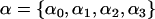denotes a vector of model parameters to be estimated. The magnitude and sign of these parameters indicate the strength and direction of the effect of the corresponding biotic/abiotic factors. α₃ corresponds to the interaction of the two factors. To improve computational efficiency and facilitate the posterior interpretation process, the factors should be normalized so as to have mean 0 and variance 1. The variance of the lognormal distribution, σ², is a measure of model fit and has to be estimated too. To estimate this and all other parameters related to the effect of environmental factors, we use vague priors. More specifically, we take 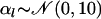and .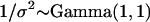

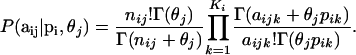
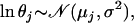
With these likelihoods and priors, the full posterior distribution represented by the directed acyclic graph (DAG) in Figure 1 is given by

(6)

Figure 1.—

The DAG of the model given in Equation 6. Square nodes denote known quantities (i.e., data) and circles represent parameters to be estimated. Lines between nodes represent direct stochastic relationships within the model. The variables within each node correspond to the different model parameters discussed in the text. A is the genetic data and G the environmental data used to explain the genetic differentiation. is the matrix of ancestral allele frequencies, is the vector of the genetic differentiation coefficient for each local population, is the vector of regression coefficients that correspond to factors in G, and σ² measures the deviation from the regression. The multinomial-Dirichlet distribution allows the exact calculation of the marginal likelihood to eliminate the nuisance parameters .

Posterior model probabilities:

As well as parameter estimates, we are interested in determining the dependence (or otherwise) of the factors upon the genetic differentiation. Alternative models are obtained by adopting different forms for μ_j given in Equation 5. The simplest model might set μ_j = α₀, corresponding to the assumption that neither factor has an effect upon the genetic differentiation. A suitable alternative might be 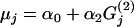, in which we assume that factor G⁽²⁾ has some influence. Clearly these models can be expressed by setting the appropriate α_l = 0 in Equation 4 with the obvious restriction that the interaction term can be included only if both G⁽¹⁾ and G⁽²⁾ are included in the model. Thus with two environmental factors there are nine alternative models as shown in Table 1 for the human example (see below).

TABLE 1.

Posterior model probabilities

Model	Factors included	Probability
1	Constant	0
2	Latitude	0
3	Constant and latitude	0
4	Longitude	0
5	Constant and longitude	0
6	Latitude and longitude	0
7	Constant, latitude, and longitude	0.97
8	Latitude, longitude, and interaction	0
9	All	0.03

Posterior probabilities of the nine possible models are shown to explain the genetic differentiation in humans as a function of latitude and longitude. We used an uniform prior for model probabilities.

To discriminate between the different models we let denote the vector of nonzero α-values under model M and then derive the following posterior distribution over both parameter and model space,

(7)

where p(M) denotes the prior model probability. In most cases, it makes sense to use a uniform prior where all models are equally likely, so this is the strategy we adopted for all the analyses that follow.

Implementation:

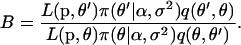
The estimation of model parameters is carried out using a combination of Markov chain Monte Carlo (MCMC) and reversible-jump MCMC (RJMCMC) (Green 1995) techniques that are described in appendix a. We evaluated the convergence of the method using the diagnostic tests implemented in the R BOA package (Bayesian Output Analysis Program version 1.1.5, Smith 2005). The tests indicated that a burn-in of 2000 iterations was enough to attain convergence and it has been implemented as part of the pilot-tuning process (see appendix a). We used a sample size of 10,000 and a thinning interval of 10 as suggested by an autocorrelation analysis. With these parameter values, the total length of the chain was 100,000 iterations. Posterior model probabilities are estimated from the number of times the algorithm visited each model. F_ST's are estimated using model-averaged posterior means and, therefore, take into account model uncertainty. The parameters of the linear model, and σ², are specific to each model and, therefore, we report the estimates obtained for the model with the highest posterior probability. Additionally, instead of using the posterior means of σ² we use its mode because its posterior density is highly asymmetric.

SIMULATION STUDY

We evaluate the performance of the method using three different approaches to generate simulated data. The first approach uses the same statistical model assumed by our method (the inference model) and allows us to study the effect of the quality of the samples (number of loci, sample sizes) and different biological scenarios (number of populations, environmental factors considered, etc.) on the accuracy of the estimates obtained. The two other approaches allow us to explore the performance of the method under scenarios that deviate from the assumptions of the inference model. We used EasyPop (Balloux 2001) to generate data under a migration–drift–mutation model that incorporates the effect of isolation by distance and SPLATCHE (Currat et al. 2004) to generate data under a population fission where new populations are formed progressively from older populations.

Inference model:

The inference model used to derive our method applies to two different scenarios, an island model at migration–drift equilibrium and a simple population fission model. The same algorithm can be used to generate synthetic samples under these two scenarios and is described in appendix b. We chose a set of default values for the key parameters of the inference model (see Table 2) and first evaluated the accuracy of the method using the relative mean square error (RMSE),

where is its true value of the parameter being estimated and p_k is its estimated value for replicate k. We analyzed 10 replicate data sets generated using the default values (Table 2). We considered samples of good quality (50 individuals and 20 loci) but within the range of those commonly seen in the literature. We also studied the effect of changing the value of one parameter at a time. We used data simulated under model 7 that include two factors and a constant term. The degree of uncertainty of the estimations is measured by the 95% highest probability density interval (HPDI, the smallest interval that contains 95% of the values).

TABLE 2.

Default parameters

Parameter	Value
Populations	10
Loci	20
Sample size per population	50
Mean no. of alleles	10
Mean FST	0.1
Model	7
α0	−2.4
α1	−0.6
α2	0.5
σ2	0.1

Default parameters used in data simulated under the inference model discussed in text are shown.

Accuracy:

In general, all estimates have a small RMSE and narrow HPDI with the exception of σ² (Table 3). Lower values of F_ST lead to slightly higher RMSEs. The poor estimation of σ² is due to the uncertainty in the estimation of the α's, which cannot be separated from the deviation from the regression included in the model. As is shown below, the quality of the estimation for this parameter can be greatly improved by increasing the number of populations sampled.

TABLE 3.

Accuracy of the estimates

Parameter	True value	Estimated value	RMSE (%)	95% HPDI
	0.101	0.111	2.8	[0.087; 0.136]
	0.100	0.107	2.1	[0.083; 0.131]
	0.146	0.151	0.8	[0.121; 0.184]
	0.072	0.076	1.0	[0.058; 0.095]
	0.029	0.031	4.3	[0.022; 0.042]
	0.036	0.041	5.3	[0.029; 0.053]
	0.236	0.247	0.7	[0.203; 0.295]
	0.112	0.111	0.4	[0.086; 0.136]
	0.029	0.034	7.9	[0.024; 0.045]
	0.180	0.183	1.3	[0.149; 0.224]
σ2	0.10	0.245	167.3	[0.095; 0.678]
α0	−2.40	−2.310	0.2	[−2.683; −1.943]
α1	−0.60	−0.553	1.1	[−0.916; −0.200]
α2	0.50	0.495	0.5	[0.142; 0.843]

Estimations, RMSEs, and 95% HPDIs based on 10 replicates simulated under the inference model. Estimated values correspond to the posterior means with the exception of σ², which is estimated by the mode. See Table 2 for parameter values used.

Sample sizes and number of loci:

The quality of the estimates is good even with the lowest sample size and number of loci (Tables 4 and 5) and increases as they increase, especially for estimates of F_ST. The posterior probability of the true model (7) was always the highest, independently of sample size and number of loci but model determination did increase substantially as they increased. The second most probable model always had a probability at least three times lower than that of the true model. Note that it is easier to improve estimates (i.e., decrease HPDIs and increase posterior probability of the true model) by increasing the number of loci studied than by increasing sample sizes. In particular, increasing sample sizes beyond 50 does not improve estimates.

TABLE 4.

The effect of sample sizes on quality of estimation

		Sample size per population
Parameter	True value	10	20	50	100
	0.101	0.106	0.133	0.109	0.098
		[0.069; 0.144]	[0.101; 0.171]	[0.085; 0.134]	[0.078; 0.120]
	0.100	0.105	0.085	0.110	0.111
		[0.068; 0.141]	[0.061; 0.111]	[0.085; 0.135]	[0.089; 0.134]
	0.146	0.156	0.160	0.170	0.128
		[0.109; 0.201]	[0.122; 0.200]	[0.137; 0.206]	[0.103; 0.154]
	0.072	0.100	0.085	0.084	0.080
		[0.065; 0.138]	[0.060; 0.110]	[0.066; 0.105]	[0.063; 0.097]
	0.029	0.033	0.031	0.025	0.032
		[0.014; 0.054]	[0.019; 0.044]	[0.017; 0.034]	[0.024; 0.041]
	0.036	0.044	0.036	0.044	0.032
		[0.022; 0.067]	[0.022; 0.051]	[0.031; 0.057]	[0.024; 0.041]
	0.236	0.207	0.281	0.251	0.231
		[0.149; 0.265]	[0.221; 0.342]	[0.206; 0.299]	[0.191; 0.273]
	0.112	0.117	0.137	0.121	0.095
		[0.079; 0.157]	[0.102; 0.173]	[0.094; 0.148]	[0.076; 0.115]
	0.029	0.037	0.035	0.045	0.031
		[0.017; 0.059]	[0.021; 0.051]	[0.033; 0.057]	[0.024; 0.040]
	0.180	0.167	0.139	0.212	0.196
		[0.120; 0.218]	[0.104; 0.175]	[0.171; 0.254]	[0.161; 0.232]
σ2	0.10	0.229	0.243	0.246	0.233
		[0.095; 0.673]	[0.096; 0.704]	[0.096; 0.708]	[0.094; 0.655]
α0	−2.40	−2.31	−2.30	−2.24	−2.38
		[−2.70; −1.91]	[−2.67; −1.90]	[−2.63; −1.88]	[−2.73; −2.03]
α1	−0.60	−0.507	−0.607	−0.576	−0.525
		[−0.876; −0.126]	[−0.976; −0.228]	[−0.941; −0.190]	[−0.887; −0.201]
α2	0.50	0.470	0.473	0.487	0.533
		[0.109; 0.817]	[0.107; 0.817]	[0.144; 0.843]	[0.192; 0.887]
p(M = 7)		0.59	0.72	0.80	0.80

True values, estimated values, and 95% HPDIs from simulated data for various sample sizes. Estimated values correspond to the posterior means with the exception of σ², which is estimated by the mode. The last line presents the posterior probability of the true model, p(M = 7). See Table 2 for parameter values used.

TABLE 5.

The effect of the number of loci studied on the quality of the estimates

		No. of loci
Parameter	True value	10	20	50
	0.101	0.089	0.109	0.096
		[0.062; 0.119]	[0.085; 0.134]	[0.083; 0.111]
	0.100	0.085	0.110	0.109
		[0.057; 0.114]	[0.085; 0.135]	[0.094; 0.126]
	0.146	0.143	0.170	0.150
		[0.104; 0.184]	[0.137; 0.206]	[0.1305; 0.1711]
	0.072	0.076	0.084	0.070
		[0.052; 0.102]	[0.066; 0.105]	[0.059; 0.081]
	0.029	0.041	0.025	0.041
		[0.026; 0.059]	[0.017; 0.034]	[0.033; 0.048]
	0.036	0.043	0.044	0.041
		[0.027; 0.061]	[0.031; 0.057]	[0.034; 0.048]
	0.236	0.186	0.251	0.243
		[0.136; 0.236]	[0.206; 0.299]	[0.214; 0.273]
	0.112	0.118	0.121	0.120
		[0.083; 0.153]	[0.094; 0.148]	[0.103; 0.137]
	0.029	0.020	0.045	0.034
		[0.010; 0.030]	[0.033; 0.057]	[0.027; 0.041]
	0.180	0.150	0.212	0.175
		[0.107; 0.194]	[0.171; 0.254]	[0.152; 0.199]
σ2	0.10	0.252	0.246	0.230
		[0.105; 0.737]	[0.096; 0.708]	[0.100; 0.613]
α0	−2.40	−2.449	−2.24	−2.31
		[−2.831; −2.038]	[−2.63; −1.88]	[−2.65; −1.96]
α1	−0.60	−0.529	−0.576	−0.509
		[−0.892; −0.151]	[−0.941; −0.190]	[−0.857; −0.198]
α2	0.50	0.458	0.487	0.468
		[0.100; 0.843]	[0.144; 0.843]	[0.154; 0.799]
p(M = 7)		0.48	0.80	0.80

True values, estimated values, and 95% HPDIs from simulated data sets with different numbers of loci are shown. Estimated values correspond to the posterior means with the exception of σ², which is estimated by the mode. The last line presents the posterior probability of the true model, p(M = 7). See Table 2 for parameter values used.

Number of populations:

Varying the number of populations changes the number of F_ST-values considered in the model; therefore, we evaluate only its effect on model determination and on estimates of regression parameters. With only 5 or 7 populations the method fails to identify the true model and provides low-quality estimates of regression parameters (Table 6). However, with ≥10 populations model determination greatly improves (the posterior probability for the true model is at least 0.80) and bias and uncertainty of all regression parameter estimates decrease pronouncedly. This is particularly the case for σ²-estimates, in which bias almost disappears with 20 populations. The results obtained depend largely on the values chosen for the coefficients of the regression (α₀ = −2.4, α₁ = −0.6, and α₂ = 0.5). The effect of a factor on population genetic structure is proportional to the absolute value of the corresponding regression coefficient. Factors with a strong effect are more easily identified than factors with a small effect. Thus, with only five populations, the highest posterior probability corresponds to the model with the constant term only. With 7 populations, the method can also identify the effect of the first factor but not that of the second and, therefore, the posterior probability is highest for model 5. The effect of the second factor is identified only with ≥10 populations. Additionally, models that do not include the constant term are readily excluded because its effect is very strong and easily identified by the method. It is important to note that when the method fails to identify the true model, the results obtained give hints that they are not reliable. For instance, the posterior probability of models with either factor is nonnegligible (>15%) and the estimates of σ² are very high (upper bound of the HPDI well over 1). Thus alert users of the method will not be misled to accept a false model; instead they will conclude that the results are inconclusive.

TABLE 6.

The effect of the number of populations studied on the quality of the estimates

		No. of populations
Parameter	True value	5	7	10	20
α0	−2.4	−2.67	−2.15	−2.23	−2.33
		[−3.23; −1.40]	[−2.80; −1.50]	[−2.63 ; −1.88]	[−2.52; −2.15]
α1	−0.6	a	a	−0.57	−0.60
		a	a	[−0.941; −0.190]	[−0.783; −0.423]
α2	0.5	a	0.67	0.46	0.49
		a	[0.059; 1.25]	[0.144; 0.843]	[0.311; 0.670]
σ2	0.1	0.67	0.51	0.25	0.12
		[0.203; 2.84]	[0.152; 1.71]	[0.096; 0.708]	[0.065; 0.261]
Model 1		0.53	0.17	0.01	0
Model 2		0	0	0	0
Model 3		0.22	0.22	0.11	0
Model 4		0	0	0	0
Model 5		0.16	0.32	0.02	0
Model 6		0	0	0	0
Model 7		0.08	0.26	0.80	0.97
Model 8		0	0	0	0
Model 9		0.01	0.03	0.06	0.03

True values, estimated values, 95% HPDIs, and posterior model probabilities from simulated data sets with different numbers of populations are shown. Estimated values correspond to the posterior means with the exception of σ², which is estimated by the mode. Posterior model probabilities are estimated from the number of times the algorithm visited each model. Models not shown are never visited by the chain. See Table 2 for parameter values used.

^aData sets in which the highest probability model does not include the corresponding parameter.

Model determination:

We simulated data under all models except equivalent ones (e.g., model 3 and model 5). The true model has always the highest probability. We note that this probability seems to increase with the number of parameters included in the true model. The probabilities of the true models are, respectively, 0.86, 0.82, 0.91, 0.70, 0.80, 0.93, and 1.00 for models 1, 2, 3, 6, 7, 8, and 9.

Overall the results of these simulations indicate that the method can accurately estimate the parameters and identify the true model if samples are of at least average quality.

Subdivided population model:

The first interpretation of our inference model (see above) considers a subdivided population at migration–drift equilibrium where the proportion of migrants can differ among local populations but where all migrant groups are drawn from the same migrant pool (see Balding 2003). Here we consider instead an isolation-by-distance scenario where the composition of the migrant group arriving at any local population depends on the distance between the focal population and each one of the other local populations. Synthetic data for this scenario can be generated using EASYPOP, a software that implements an individual-based model for the simulation of genetic data under different scenarios of population subdivision. We considered a scenario with 14 local populations, each consisting of 50 individuals (see Figure 2A). The probability of being a migrant was fixed to 0.05 and the migration rate between populations followed a negative exponential kernel with parameter r = 1/α. Thus, when the populations are totally isolated and as α increases, the effect of distance on migration rates decreases; here we take α = 0.75. We simulate 15 loci, each with six allelic states and with a mutation rate of 0.0001. Using these settings we generated 10 replicate data sets consistent with a scenario where population genetic structure is influenced only by the degree of geographic isolation of local populations, which is measured by their connectivity. This measure is typically used in metapopulation studies to describe the effect of the habitat matrix properties on the degree of isolation of local populations (e.g., Moilanen and Nieminen 2002). There are many connectivity measures to choose from, and some include geographic distance and habitat patch size and shape. Since we consider only the degree of geographic isolation we chose to use the connectivity of population j, S_j,

where d_ij is the distance between populations j and i, and β measures the effect of distance on migration probability.

Figure 2.—

(A) Map of the 14 populations used for the isolation-by-distance model simulated with EASYPOP. The connectivity of each population is described by the shaded scale. Populations with dark shading are isolated while ones with light shading are well connected to others. (B) Plot of ln[F_ST/(1 − F_ST)] against the connectivity for the isolation-by-distance simulated data. The equation of the regression line is ln[F_ST/(1 − F_ST)] = −1.12 − 0.50S, where S denotes the connectivity measure defined in the text.

The analyses of these data sets consider three alternative models, a null model that includes the constant regression term (model 1), another that includes only connectivity (model 2), and finally a model that includes both the constant term and the distance (model 3).

Our method correctly identifies model 3 as the most probable with a posterior probability of 0.90. The regression coefficients α₀ and α₁ are estimated, respectively, as −1.12 and −0.50. More isolated populations (e.g., 1, 2, or 8) have a higher F_ST than well-connected populations (e.g., 3, 4, or 5). The connectivity explains relatively well the genetic differentiation because the posterior mode of σ² is 0.24 and there is little scattering of points around the regression line (Figure 2B). These results indicate that the method provides reliable results under an isolation-by-distance model applicable to a wide range of species.

Spatial population expansion model:

The second interpretation of our inference model considers a simple fission scenario where local populations evolve in isolation after splitting from an ancestral population. To evaluate the performance of the method when the true evolutionary model differs radically from this scenario we used SPLATCHE (Currat et al. 2004). More specifically, SPLATCHE simulates a population expansion from a single origin in a two-dimensional habitat (strict two-dimensional stepping-stone model) and generates genetic samples for geographic locations chosen by the user. We used the example of the human population expansion with origin in East Africa (see below) as a template for our simulated scenarios. We used a growth rate of 0.10, a carrying capacity of 100 for all demes, and a migration rate of 0.20. With these settings, the whole world is colonized after ∼4000 generations. We simulated 10 replicates of this scenario and for each of them we “collected” genetic data for 36 populations chosen uniformly on the map (Figure 3 shows the map of the world with the sampling locations). We calculated the distance from East Africa to each of the sampling locations using the shortest possible land-based route. The objective of this part of the study is to determine if our method can detect the genetic signal left by a recent spatial population expansion so we use distance from East Africa as a factor in our analysis. However, we also include a second factor, “insularity,” to illustrate the flexibility of our method. Clearly, genetic structure is influenced by physical barriers to migration such as water masses. Therefore, the second factor considered by the logistic regression model (4) takes values of either 0 for continental populations (e.g., those in mainland Europe, Africa, Asia, and America) or 1 for insular populations (those in England, Japan, Indonesia, New Zealand, Australia, and Greenland).

Figure 3.—

Map of the 36 populations (shaded circles) used in the simulation of the colonization of the world with SPLATCHE. The solid square indicates the origin of the expansion.

The results of this analysis clearly show that our method can accurately detect the effect of not only distance but also other physical barriers despite the fact that the synthetic data were generated using a demographic model that differs radically from the simple fission model. Figure 4 shows the plots of ln[F_ST/(1 − F_ST)] vs. distance and insularity. Data points correspond to mean values over the 10 replicated scenarios. The posterior probability of the model with the constant factor and both distance from East Africa and insularity is 0.97. Figure 4 shows the strong effect of distance on F_ST and it also indicates that insular populations (identified with triangles) would not fit very well the regression line without including the insularity factor. Here we estimate σ² = 0.15 while in another analysis without the insularity factor we obtained σ² = 0.25.

Figure 4.—

Plots of ln[F_ST/(1 − F_ST)] against the two factors, distance to East Africa and insularity, for the human simulated data. Triangles indicate insular populations and solid squares indicate African populations. The equation of the regression line is ln[F_ST/(1 − F_ST)] = −2.59 + 0.46d, where d denotes the distance to East Africa.

APPLICATIONS

Argan tree:

One of the goals of conservation genetics is to identify populations for on-site conservation. This requires the characterization of the status of each local population in terms of its genetic diversity and its degree of differentiation with respect to all other populations and an understanding of the factors that are responsible for the observed genetic structuring. A good example of this type of study is presented by Petit et al. (1998), who analyzed the genetic structure of the argan tree of Morocco. Here we use their data to illustrate how our approach can be applied to study metapopulation scenarios with the objective of determining if the degree of isolation is influenced by geographic location and/or one other factor, in this case altitude. We note that this latter variable was not considered by Petit et al. (1998) and is included here only for the sake of illustration.

Data:

The argan tree data consist of samples from 12 populations that were analyzed for 12 polymorphic loci. Sample size varied between 20 and 50 individuals per population. Geographic isolation of each local population is modeled using two factors, connectivity and elevation. Connectivity was calculated using the geographic distance between populations (kindly provided by R. Petit) and the same connectivity measure, S_j, as in the simulation study (see above). The elevation data were obtained from Table 1 in Petit et al. (1998).

Results:

The highest probability model (P = 0.60) includes a constant and connectivity. This model dominates well all the others, and it seems clear that elevation does not influence genetic differentiation since models that include this factor have low posterior probability (between 0 and 0.07). The estimated σ² is 0.27 (HPDI = [0.13; 0.82]), which indicates that distance explains well the genetic differentiation and that, although some other unknown environmental factor may also play a role, its effect is unlikely to be very strong. The estimate of α₂ = −0.55, which is negative, indicating that genetic differentiation does indeed increase with increasing geographic isolation (see Figure 5).

Figure 5.—

Plots of ln[F_ST/(1 − F_ST)] against the connectivity for the argan tree data. The equation of the regression line is ln[F_ST/(1 − F_ST)] = −0.66 − 0.55S, where S denotes the connectivity measure defined in the text.

Humans:

One of the most widely accepted theories on the origin of modern humans, the recent African origin (RAO) model, postulates that our species has evolved from a small East African population that had subsequently colonized the whole world. Numerous studies provide evidence supporting this model but less is known about the specific details of the demographic history of humans (see Excoffier 2002). For example, some studies have found that an important component of human diversity seems to have evolved outside Africa (Zhao et al. 2000; Yu et al. 2001), which has been interpreted as implying a migration back to Africa. Also, the strength of the bottlenecks that may have taken place in the colonization process and the magnitude of the subsequent population expansions remain controversial (see Excoffier 2002 for a review). Here we use the Human Genome Diversity Cell Line Panel–Centre d'Etude du Polymorphisme Humain (HGDP–CEPH) presented by Cann et al. (2002) to illustrate how our method can be used to make inferences about population expansion events such as those undergone by humans.

Data:

The data consist of 1056 individuals from 51 subpopulations, which were scored for 377 microsatellites. We carried out two analyses. The first one considers the effect of one factor, geographic distance from East Africa along colonization routes (as in Prugnolle et al. 2005), while the second one considers a model with two factors, longitude and latitude.

Results:

Estimated F_ST-values are presented in appendix c. If humans spread from East Africa and in the process underwent successive bottlenecks of small amplitude (as proposed by Prugnolle et al. 2005) we should expect a gradual increase in F_ST-values as the distance from the center of origin increases. Thus, we followed Prugnolle et al. (2005) and calculated the distance from East Africa along likely colonization routes for each one of the 51 populations and estimated the posterior probability of the three alternative models, with and without distance. The estimated posterior probability of the model with the constant factor and distance is 1. Figure 6 shows the strong effect of distance on θ but it also indicates that some of the African populations (identified by solid squares) do not fit very well the regression line. Indeed, repeating the estimation process without these populations improves the fit from σ² = 0.27 to σ² = 0.18. Several factors can explain the relative lack of fit of African populations (see discussion).

Figure 6.—

Plots of ln[F_ST/(1 − F_ST)] against the distance to East Africa for the human data. Solid squares indicate African populations. The equation of the regression line is ln[F_ST/(1 − F_ST)] = −3.01 + 0.56d, where d denotes the distance to East Africa.

Another way of uncovering the genetic signature left by the demographic history of humans is to carry out a second analysis that uses as factors latitude and longitude. The rationale for this is that under the RAO model there should be a clear effect of longitude on F_ST since the most important population movements have occurred along this axis (e.g., Piazza et al. 1981). We also expect an effect of latitude due to the combined effect of southward population movements (mainly in the Americas but also in Africa), climate, and smaller effective sizes of the southern populations included in the data set (the African and Amerindian populations are much smaller than the European and most Asian populations). Thus, latitude would take into account the increased effect of genetic drift due to all these factors.

To take into account the fact that the Americas were colonized from East Asia, we measured longitude on a scale between 0° and 360° from west to east and starting at the Greenwich meridian. With the two factors considered, there are nine alternative models but almost all the probability mass was allocated to model 7 (Table 1) that includes the constant term and both latitude and longitude. The only other model visited is model 9 with probability 0.02, which also includes the two factors. So it is clear that they both play a major role in explaining the observed genetic structure. In addition, the estimate of σ² is 0.19 with a HPDI of [0.13; 0.29], yet another indication that these two factors explain well the observed genetic pattern. Note also that this estimate of σ² is lower than that obtained above for the analysis that included the African populations and is almost identical to that obtained excluding these populations. Thus, latitude and longitude explain more of the variation than distance alone. The stronger effect of longitude is indicated by the larger absolute value of its regression coefficient (see Table 7) and the less pronounced scattering of points in the plot of ln[F_ST/(1 − F_ST)] against longitude than against latitude (Figure 7). The negative value of α₂ indicates that colonization occurred mainly from west to east while the negative value of α₁ indicates that the effect of genetic drift was stronger in the southern populations.

TABLE 7.

Human data regression

Parameter	Factor	Mean	95% HPDI
α0	Constant	−3.01	[−3.13; −2.88]
α1	Latitude	−0.30	[−0.44; −0.18]
α2	Longitude	−0.43	[−0.56; −0.30]

Estimation of α_l regression coefficients with 95% HPDIs is shown.

Figure 7.—

Plots of ln[F_ST/(1 − F_ST)] against the two factors: latitude and longitude for the human data.

DISCUSSION

In this article we present a new Bayesian method to evaluate the effect that biotic and abiotic environmental factors (geographic distance, language, temperature, altitude, local population sizes, etc.) have on the genetic structure of populations. It estimates F_ST-values for each local population and relates them to environmental factors using a generalized linear model. The method requires genetic data from codominant markers (e.g., allozymes, microsatellites, or SNPs) and environmental data specific to each local population. The results of our simulation study indicate that the method can correctly identify the environmental factors that influence the structuring of genetic variability under a wide range of conditions. In particular, it can perform very well for moderate values of sample sizes (20) and number of loci (10) and it is very robust to deviations from the inference model assumed by our method. Thus, it should be applicable to a wide variety of species.

Our method provides many pieces of information that can help us better understand the demographic and evolutionary history of the species under study. Population-specific F_ST's allow us to establish how distinct a local population is in terms of its genetic composition; a high F_ST indicates that the allele frequency distribution of a local populations is fairly different from that of the metapopulation as a whole. The posterior model probabilities allow us to identify the biotic/abiotic factors controlling genetic structure and also explain why a given local population is or is not genetically distinct. The signs of the regression coefficient estimates indicate if the effect of a factor increases or decreases genetic differentiation and, when the most probable model includes more than one factor, their absolute value tells us which factor has a stronger effect.

The method can be used to study a wide range of problems, including human genetics, conservation biology, and species demographic history. In the field of human genetics it can be used to test for the importance of cultural factors as descriptors of the distribution of genetic variation in humans. This information is of fundamental importance for efforts to identify disease genes by association with marker loci. In the field of conservation biology, the identification of the factors that are important determinants of the genetic structure of natural populations can help design management strategies for best preserving genetic biodiversity. It can also help gather valuable information for designing and parameterizing simulation models aimed at predicting the effect of global climate change on natural populations. Its application to the study of population demographic history is well illustrated by the application of our method to the analysis of the HGDP–CEPH Human Genome Diversity Cell Line Panel (see below).

As opposed to the multivariate Mantel test, which uses a summary statistic (pairwise genetic distance), our method is model based and makes full use of the data (allele frequencies). This is a very important consideration when data sets are not very large, as is usually the case. Additionally, it avoids the problems faced by many frequentist approaches, most of which use randomization techniques to test for the significance of the relationships. In the particular case of the multivariate Mantel test, Raufaste and Rousset (2001) and Rousset (2002) have recently called into question the validity of the jackknife procedure when two or more environmental factors are included in the analysis. The limitations of the sequential testing procedures were discussed previously by Cheverud et al. (1989) and particularly by Legendre (2000), who described two additional randomization methods for carrying out the multivariate Mantel test. Legendre (2000) also provided recommendations on ways of deciding which randomization technique is more appropriate for the data at hand. Thus, the multivariate Mantel test can be used as a data exploration technique provided that all these considerations are taken into account. On the other hand, a more information-rich method, such as ours, is more suitable when the aim is to test specific hypotheses about the effect of environmental factors. It is also more appropriate for studying the influence of variables whose effects cannot be measured in terms of pairwise distance measures. For example, the effect of local population sizes on genetic structuring cannot be modeled using pairwise distances since the effect of genetic drift is determined by the N_e of each local population and not by their difference. Our approach can readily account for this effect if estimates of local population sizes are available. Also, as shown in our simulation study, it can be used to study the effect of physical barriers such as water masses by considering a binary factor to discriminate between, for example, continental and insular populations.

The generality of our method stems from the fact that the likelihood function we use arises as an approximation to two different demographic models. In the case of the fission model considered by Nicholson et al. (2002) and Falush et al. (2003), the population-specific F_ST's measure the degree of genetic differentiation between each descendant population and the ancestral population. In the case of the island model considered by Balding and Nichols (2005) and Balding (2003), the F_ST's measure how divergent each local population is from the metapopulation as a whole. In both cases, the estimation of individual F_ST's for each one of the descendant/local populations takes into account the fact that the strength of genetic drift differs among them, something that is overlooked by the traditional procedure of estimating a single F_ST-value for the whole set of demes.

We illustrate the application of our method using published data sets. The argan tree example approaches a migration–drift model and uses connectivity and altitude as factors that could explain the genetic structuring. There is no a priori reason to believe that altitude plays a role and our method confirms this expectation. Connectivity on the other hand has a strong effect. Although our example considers only abiotic factors, it is also possible to include biotic factors directly related to dispersal, for example, the abundance of a pollinator species.

The human example illustrates the application of our method to a scenario that approaches imperfectly that of a fission model. Our analysis of the effect of distance to East Africa on F_ST-values (Figure 6) is not entirely consistent with those obtained by Prugnolle et al. (2005), who considered its effect on heterozygosity. In our case, although the overall fit of the model is very good, three African populations (Biaka Pigmies, Mbuti Pygmies, and San) seem to deviate more from the F_ST-values predicted by distance. This distinct behavior of African populations has also been observed by Ramachandran et al. (2005), using regression methods that did not explicitly assume a specific evolutionary model (but see below). Several factors can explain this lack of fit. The first one to consider is a mismatch between the fission model assumed by the method and the real demographic history of humans. Indeed, the fission model assumes that all subpopulations evolved from an ancestral population while the RAO model considers a series of bottlenecks with new populations being formed progressively from the ones that left the ancestral population. To determine if this is the source of the problem, we used SPLATCHE (Currat et al. 2004) to generate synthetic data under the RAO model (see results). The simulations considered a population expansion from a single origin in East Africa in a two-dimensional habitat (strict two-dimensional stepping-stone model) and collected genetic data for 36 populations chosen uniformly on the map (cf. Figure 3). As we did in the analysis of the real data set, we use distance from East Africa as a factor but also added a second factor, insularity, to account for the barrier effect of water masses, which was expected to be very strong due to the way migration across water masses has to be modeled with SPLATCHE. The results (Figure 4) show that samples collected in Africa are no longer outliers, indicating that the mismatch between the inference model and the RAO model is unlikely to be responsible for the observed lack of fit.

Another potential explanation for the lack of fit of African populations is that they may have smaller effective sizes, a consequence of being rather small and isolated tribal groups. In their analysis, Prugnolle et al. (2005) used heterozygosity, a summary statistic that does not really take into account the information provided by very low-frequency alleles. Thus, it is less affected by genetic drift due to small population sizes and provides a better fit. The fit of the model might have been improved by including estimates of local population sizes but no such estimates were available. Finally, a third possible explanation is a potential ascertainment bias in the choice of the microsatellites of the database we used. Indeed, these markers were primarily ascertained on an European CEPH panel and may be biased toward loci that are more variable in European than in African populations (Ray et al. 2005). This would introduce a bias in the estimation of the ancestral allele frequency distribution, which will be closer to that in European populations. Prugnolle et al. (2005) used heterozygosity, which, as mentioned before, is less sensitive to the effect of low-frequency alleles and therefore is less influenced by ascertainment bias. We carried out simulations to determine to what extent ascertainment bias can influence the results given by our method. We considered the same scenario described above, i.e., 36 populations chosen uniformly on the world map, and used SPLATCHE to generate a data set with 100 loci. From these we generated an unbiased data set by selecting at random 20 loci and a biased data set by selecting 20 loci with the highest variability in a French sample. The effect of ascertainment bias can be studied using the averaged squared residuals (average squared difference between observed and fitted values) of the African samples, which in the case of the biased data set is almost twice as high as that of the unbiased one (0.073 vs. 0.042). This result suggests that ascertainment bias could explain at least part of the lack of fit of African samples. Another important effect of ascertainment bias is to skew the estimated allele frequencies of the ancestral population toward those of the population used as a reference for choosing the markers. Thus, the lowest F_ST for the biased data set value corresponds to that of the French sample, which in the unbiased data set ranked 16th. This can have a large effect on studies that attempt to narrow down the region of Africa that was the epicenter of the human population expansion. This problem was investigated by Ray et al. (2005). They carried out realistic simulations of the genetic diversity expected after an expansion of modern humans into the Old World from different possible areas and then compared the results to the same human data set we have analyzed. Their results point toward a North African origin for modern humans. To uncover the effect of ascertainment bias they generated 20,000 data sets under the assumption of an East African origin. They then selected 1000 simulations with the highest variability in the subset of European samples (a biased data set) and 1000 additional simulations selected at random (an unbiased data set). The results obtained with the biased samples indicated a North African origin while the unbiased samples correctly pointed toward an East African origin. To take into account the effect of ascertainment bias they used synthetic data sets that presented the same bias as the real human database. With this correction, the best fit between observed and simulated data was obtained for the scenario that considered an East African origin for modern humans. A better understanding of the demographic history of humans requires a more even geographic coverage of sampling efforts and less biased choice in the selection of the loci.

A statistical problem that arises when assessing the effect of geographic distance from East Africa on human genetic diversity/differentiation is that human populations have a shared history of drift and cannot be considered as independent. For example, Amerindian populations have all issued from the same bottleneck that took place at the time of colonization of the American continent and they all bear its genetic signal. This is akin to the problem that Felsenstein (1985) pointed out for studies that use the comparative method and is common to all the recent studies that have used a regression approach to evaluate the validity of the RAO model (e.g., Prugnolle et al. 2005; Ramachandran et al. 2005; Amos and Manica 2006). More precisely, human populations can be considered as independent for the purpose of statistical analysis only under a strict fission model, in which case the history of genetic drift in the different human populations will be independent. Otherwise, populations in the different continents or regions of the globe will all bear the signal of the bottleneck at the time of colonization of that particular continent/region. Thus, samples coming from the same geographical area can be considered, to at least some degree, as replicates and may inflate the statistical significance of the regression. Although we use a Bayesian approach, our method does not avoid this problem so we carried out simulations to try to evaluate to what extent this lack of independence can affect the results. The Amerindian populations are the most likely to influence the estimates of σ², the variance of θ's, and the posterior model probabilities. Thus, we compared the results of three different scenarios that differ in the number of Amerindian samples. In the first scenario samples were collected from 36 populations chosen uniformly on the world map (the unbiased scenario described above); they comprised 4 populations from North America, 1 from Central America, and 4 others from South America. The second scenario considered 29 populations in total, with only 1 each in North, Central, and South America. Finally, we considered a third scenario with 44 sampled populations of which 4 were from North America, 1 was from Central America, and 12 were from South America. The results correspond to averages across 10 independent simulations of each scenario. They indicate that the number of Amerindian samples included has little effect on posterior model probabilities (0.97 for scenario 1, 0.93 for scenario 2, and 0.99 for scenario 3) and the estimates of σ² (0.15, 0.18, and 0.13, respectively). Duplicated populations can also have an effect similar to that of ascertainment bias (i.e., skew ancestral allele frequencies toward those of European populations) if a large number of samples are from Europe and the Middle East. We explored this issue using simulations of a scenario where we added six European samples to the unbiased data set. In this case, the estimated posterior probability of model 7 is 1 and the estimate of σ² is 0.17, indicating that the effect is rather weak. Additionally, the average F_ST of European populations for the data set with more European samples (F_ST = 0.059) is almost the same as that obtained for the unbiased one (F_ST = 0.061). Ideally one would like to eliminate all nonindependent samples as we did for the American continent but it is not clear how to identify the duplicated samples for large areas such as Asia, without knowing the history of the bottlenecks. In any case, the results of the simulations suggest that despite this problem our method seems capable of correctly identifying the effect of distance or other factors on genetic differentiation when the true model radically differs from the fission model.

The results of the application of our method to the study of human demographic history seem to suggest a rapid population expansion into the Middle East and Europe as indicated by the low F_ST-values obtained for all the populations in these regions. Indeed, under a rapid population expansion, the effect of genetic drift is greatly reduced, leading to low F_ST-values. This rapid expansion seems to have been followed by a slower expansion into East Asia, Australasia, and the Americas. There are clear longitudinal and latitudinal gradients in the degree of genetic differentiation of subpopulations (Figure 7), with values of F_ST increasing both toward the east and toward the south, but with a stronger effect of longitude. This is expected because most population movements occurred along a west–east axis. Equivalent results were obtained by the seminal work of Piazza et al. (1981) in a much earlier study that considered only aboriginal populations.

As opposed to the complexity of frequentist multivariate techniques such as principal component analysis or discriminant correspondence analysis, which provide results that are difficult to interpret, our Bayesian method provides results that are easy to interpret. It can be applied to the identification of the environmental factors that underlie observed spatial patterns of genetic diversity but it can also be used to study spatial population processes, such as range expansions, by simply introducing longitude and latitude as the explanatory variables. All these characteristics should make it a very valuable tool for addressing a wide range of problems.

APPENDIX A: MCMC METHODS

The RJMCMC algorithm is used to estimate the posterior probability of the alternative models and their parameters. RJMCMC updates (Green 1995) provide a natural extension to the basic Metropolis–Hastings algorithm to allow moves that change the dimension of the state vector. The estimates of model probabilities are obtained by simply observing the number of times that the chain visits each distinct model. A very thorough sensitivity study has been made to study the convergence of the method and the accuracy of the estimates under different data set scenarios (sample sizes, number of loci and populations, etc.).

Updating p:

The frequencies are updated one locus at a time. In each case, the move is accepted with probability , where

The elements of the vector are updated pairwise because they must sum to one. Thus, we select at random two different alleles m and n by choosing m uniformly from {1, … , K_i} and then choosing n uniformly from the remaining integers {1, … , K_i}\{m}. is the vector with and replaced by and . Note that for the elements to sum up to one, + = + . Thus, we first take = u, where and e is some increment value that can be pilot tuned to obtain reasonable acceptance rates. Finally, we set = + ( − ).

Updating α:

The coefficients are updated one at a time. is the vector with element α_l replaced by α′_l. The move is accepted with probability , where

We take the proposal value α′_l = α_l + e, where . Since the proposal normal density is symmetric, and thus, both terms drop from the expression for B.

Updating θ:

The θ_j's are updated one at a time. is the vector with element θ_j replaced by θ′_j. The move is accepted with probability , where

We take the proposal value ln θ′_j = ln θ_j + e, where . So we have 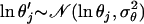and here the move is not symmetric because of the log transformation: .

Updating σ²:

We take the proposal value ln σ′² = ln σ² + e, where and the move is accepted with probability α(σ², σ′²) = min(1, B), where

Here just like for we have q(σ′², σ²)/q(σ², σ′²) = σ′²/σ².

Between-model moves:

When moving between models, we add or delete one element to the -vector. We randomly select one of these parameters and if it is already in the model, we propose to delete it. If it is not in the current model, we propose to add it. We use the canonical jump function so that when moving to a space of higher dimension (model 5 to model 7, for example) we keep the current values and we propose the new value from a distribution q. The reverse move is achieved by just deleting the parameter no longer included. Suppose we propose to add α₂ to the model and that we draw α₂ from q. Then we accept this move with probability min(1, B), where

Because we choose the new model uniformly, the ratio of prior model probability simplifies to 1. The Jacobian is one because of the canonical jump function used. To consider the reverse move, we simply accept the move deleting α₂ with probability min(1, 1/B). All the other reversible-jump moves are similar. The problem with this proposal scheme is that we might propose to add α₁ to a model without α₃. To get around this problem, we simply reject any proposal that does not make sense (for example, α₀, α₁, α₃). The proposal distribution q is a normal distribution with its mean and variance pilot tuned to improve convergence (see below).

Tuning proposal distribution:

Proposal distributions have to be adjusted to have acceptance rates between 0.25 and 0.45. Thus, we have to adjust e for the uniform proposal of allele frequencies and the variances σ_α, σ_θ, and σ_σ for the normal proposals of α, θ, and σ. If we propose values in a very wide interval, most moves will be rejected because we will often propose values in areas of low posterior probability. On the other hand, if we propose values very close to the current value, the move will be almost always accepted. These values are tuned on the basis of short pilot runs: we run 200 iterations, and for each parameter the proposal is adjusted to reduce or increase the acceptance rate. We make 10 such pilot runs before starting the sampling, which also play the role of a burn-in period. At the same time, we can choose the proposal distribution q for the reversible jump. Brooks et al. (2003) show that the best choice is to take to be the full conditional distribution of in model M′. Because we do not know this distribution, we use the pilot run to have an estimation of the mean m_i and variance v_i for all α_l under the saturated model (which corresponds to model 9). Then we propose a new value for α_l from that is generally close to the full conditional distribution.

APPENDIX B: ALGORITHM FOR SIMULATIONS OF INFERENCE MODEL

The algorithm used in the simulations of the inference model is given below in pseudocode:

• choose factors G⁽¹⁾ and G⁽¹⁾

• choose the influence of factors α and the deviation from the regression σ²

• for each locus i in 1:I

  • choose the number K_i of possible allelic states at locus i
  • choose the alleles frequencies p_i of the ancestral population at locus i

• endfor

• for each population j in 1:J

  • calculate μ_j = α₀ + α₁G_j⁽¹⁾ + α₂G_j⁽²⁾ + α₃G_j⁽¹⁾G_j⁽²⁾
  • draw θ_j from lognormal(μ_j, σ²)
  • for each locus i in 1:I

    • draw the alleles frequencies at locus i in population j
    • from
    • choose the total number n_ij of alleles at locus i in population j
    • draw the allele count a_ij at locus i in population j from
    • 
  • endfor

• endfor

APPENDIX C: HUMAN GENETIC STRUCTURE

Estimates of F_ST for the 51 human populations with 95% HPDIs

Population	FST	95% HPDI
America	0.22
Karitiana (Brazil)	0.31	[0.27, 0.35]
Surui (Brazil)	0.40	[0.36, 0.45]
Piapoco/others (Colombia)	0.26	[0.22, 0.30]
Maya (Mexico)	0.11	[0.09, 0.12]
Pima (Mexico)	0.24	[0.20, 0.27]
Oceania	0.15
Melanesian (Bougainville)	0.16	[0.14, 0.18]
Papuan (New Guinea)	0.14	[0.12, 0.16]
East Asia	0.07
Cambodian (Cambodia)	0.077	[0.061, 0.094]
Dai (China)	0.072	[0.055, 0.089]
Daur (China)	0.072	[0.055, 0.089]
Han (China)	0.076	[0.061, 0.092]
Hezhen (China)	0.091	[0.071, 0.11]
Lahu (China)	0.11	[0.092, 0.14]
Miaozu (China)	0.079	[0.060, 0.097]
Mongola (China)	0.057	[0.042, 0.071]
Naxi (China)	0.080	[0.062, 0.099]
Oroqen (China)	0.076	[0.059, 0.094]
She (China)	0.10	[0.081, 0.13]
Tu (China)	0.061	[0.046, 0.077]
Tujia (China)	0.086	[0.067, 0.11]
Uygur (China)	0.040	[0.028, 0.052]
Xibo (China)	0.056	[0.041, 0.072]
Yizu (China)	0.069	[0.053, 0.086]
Japanese (Japan)	0.069	[0.059, 0.080]
Eurasia	0.03
Balochi (Pakistan)	0.034	[0.027, 0.041]
Brahui (Pakistan)	0.032	[0.026, 0.040]
Burusho (Pakistan)	0.027	[0.021, 0.033]
Hazara (Pakistan)	0.023	[0.018, 0.030]
Kalash (Pakistan)	0.089	[0.075, 0.10]
Makrani (Pakistan)	0.023	[0.018, 0.029]
Pathan (Pakistan)	0.026	[0.020, 0.032]
Sindhi (Pakistan)	0.025	[0.019, 0.031]
Yakut (Pakistan)	0.061	[0.051, 0.073]
Basque (France)	0.040	[0.032, 0.048]
French (France various regions)	0.034	[0.027, 0.041]
Bergamo (Italy)	0.035	[0.025, 0.045]
Sardinian (Italy)	0.047	[0.038, 0.055]
Tuscan (Italy)	0.036	[0.022, 0.050]
Orcadian (Orkney Islands)	0.037	[0.027, 0.047]
Russian (Russia)	0.035	[0.027, 0.042]
Adygei (Russia Caucasus)	0.030	[0.022, 0.038]
Druze (Israel Carmel)	0.041	[0.034, 0.047]
Palestinian (Israel Central)	0.026	[0.022, 0.031]
Bedouin (Israel Negev)	0.030	[0.025, 0.035]
Mozabite (Algeria Mzab)	0.033	[0.027, 0.039]
Sub-Saharan Africa	0.08
Biaka Pygmies (Central Africa)	0.083	[0.073, 0.093]
Mbuti Pygmies (Congo)	0.099	[0.085, 0.11]
Bantu Speakers (Kenya)	0.063	[0.050, 0.074]
San (Namibia)	0.12	[0.10, 0.15]
Yoruba (Nigeria)	0.069	[0.059, 0.078]
Mandenka (Senegal)	0.058	[0.049, 0.066]

Italics identify populations with a F_ST significatively different from others in the same geographic area.

References

- Amos, W., and A. Manica, 2006. Global genetic positioning: evidence for early human population centers in coastal habitats. Proc. Natl. Acad. Sci. USA 103: 820–824. [DOI] [PMC free article] [PubMed] [Google Scholar]
- Balding, D. J., 2003. Likelihood-based inference for genetic correlation coefficients. Theor. Popul. Biol. 63: 221–230. [DOI] [PubMed] [Google Scholar]
- Balding, D. J., and R. A. Nichols, 1995. A method for quantifying differentiation between populations at multi-allelic loci and its implications for investigating identity and paternity. Genetica 96: 3–12. [DOI] [PubMed] [Google Scholar]
- Balloux, F., 2001. EASYPOP (version 1.7): a computer program for population genetics simulations. J. Hered. 92: 301–302. [DOI] [PubMed] [Google Scholar]
- Brooks, S. P., P. Giudici and G. O. Roberts, 2003. Efficient construction of reversible jump proposal distribution. J. R. Stat. Soc. Ser. B Stat. Methodol. 65: 3–55. [Google Scholar]
- Cann, H. M., C. de Toma, L. Cazes, M. F. Legrand, V. Morel et al., 2002. A human genome diversity cell line panel. Science 296: 261–262. [DOI] [PubMed] [Google Scholar]
- Cavalli-Sforza, L. L., and M. W. Feldman, 2003. The application of molecular genetic approaches to the study of human evolution. Nat. Genet. 33: 266–275. [DOI] [PubMed] [Google Scholar]
- Cheverud, J., G. Wagner and M. Dow, 1989. Methods for the comparative analysis of variation patterns. Syst. Zool. 38: 201–213. [Google Scholar]
- Currat, M., N. Ray and L. Excoffier, 2004. SPLATCHE: a program to simulate genetic diversity taking into account environmental heterogeneity. Mol. Ecol. Notes 4: 139–142. [Google Scholar]
- Excoffier, L., 2001. Analysis of population subdivision, pp. 271–308 in Handbook of Statistical Genetics, edited by D. Balding, M. Bishop and C. Cannings. John Wiley & Sons, New York.
- Excoffier, L., 2002. Human demographic history: refining the recent African origin model. Curr. Opin. Genet. Dev. 12: 675–682. [DOI] [PubMed] [Google Scholar]
- Falush, D., M. Stephens and J. Pritchard, 2003. Inference of population structure using multilocus genotype data: linked loci and correlated allele frequencies. Genetics 164: 1567–1587. [DOI] [PMC free article] [PubMed] [Google Scholar]
- Felsenstein, J., 1985. Phylogenies and the comparative method. Am. Nat. 125: 1–15. [Google Scholar]
- Gaggiotti, O. E., S. P. Brooks, W. Amos and J. Harwoods, 2004. Combining demographic, environmental and genetic data to test hypotheses about colonization events in metapopulations. Mol. Ecol. 13: 811–825. [DOI] [PubMed] [Google Scholar]
- Geffen, E., M. J. Anderson and R. K. Wayne, 2004. Climate and habitat barriers to dispersal in the highly mobile gray wolf. Mol. Ecol. 13: 2481–2490. [DOI] [PubMed] [Google Scholar]
- Green, P. J., 1995. Reversible jump MCMC computation and Bayesian model determination. Biometrika 82: 711–732. [Google Scholar]
- Holsinger, K. E., 1999. Analysis of genetic diversity in geographically structured populations: a Bayesian perspective. Hereditas 130: 245–255. [Google Scholar]
- Hunley, K., and J. C. Long, 2005. Gene flow across linguistic boundaries in native North American populations. Proc. Natl. Acad. Sci. USA 102: 1312–1317. [DOI] [PMC free article] [PubMed] [Google Scholar]
- Legendre, P., 2000. Comparison of permutation methods for the partial correlation and partial Mantel tests. J. Stat. Comput. Simul. 67: 37–73. [Google Scholar]
- Marchini, L. R., and A. Cardon, 2002. Discussion on the meeting on ‘statistical modelling and analysis of genetic data.’ J. R. Stat. Soc. Ser. B Stat. Methodol. 64: 737–775. [Google Scholar]
- Moilanen, A., and M. Nieminen, 2002. Simple connectivity measures in spatial ecology. Ecology 83: 1131–1145. [Google Scholar]
- Nicholson, G., A. V. Smith, F. Jónsson, Ó. Gústafsson, K. Stefánsson et al., 2002. Assessing population differentiation and isolation from single-nucleotide polymorphism data. J. R. Stat. Soc. Ser. B Stat. Methodol. 64: 695–715. [Google Scholar]
- Petit, R. J., A. El Mousadik and O. Pons, 1998. Identifying populations for conservation on the basis of genetic markers. Conserv. Biol. 12: 844–855. [Google Scholar]
- Piazza, A., P. Menozzi and L. L. Cavalli-Sforza, 1981. Synthetic gene frequency maps of man and selective effects of climate. Proc. Natl. Acad. Sci. USA 78: 2638–2642. [DOI] [PMC free article] [PubMed] [Google Scholar]
- Prugnolle, F., A. Manica and F. Balloux, 2005. Geography predicts neutral genetic diversity of human populations. Curr. Biol. 15: R159–R160. [DOI] [PMC free article] [PubMed] [Google Scholar]
- Ramachandran, S., O. Deshpande, C. C. Roseman, N. A. Rosenberg, M. W. Feldman et al., 2005. Support from the relationship of genetic and geographic distance in human populations for a serial founder effect originating in Africa. Proc. Natl. Acad. Sci. USA 102: 15942–15947. [DOI] [PMC free article] [PubMed] [Google Scholar]
- Raufaste, N., and F. Rousset, 2001. Are partial Mantel tests adequate? Evolution 55: 1703–1705. [DOI] [PubMed] [Google Scholar]
- Ray, N., M. Currat, P. Berthier and L. Excoffier, 2005. Recovering the geographic origin of early modern humans by realistic and spatially explicit simulations. Genome Res. 15: 1161–1167. [DOI] [PMC free article] [PubMed] [Google Scholar]
- Rousset, F., 2001. Inferences from spatial population genetics, pp. 239–270 in Handbook of Statistical Genetics, edited by D. Balding, M. Bishop and C. Cannings. John Wiley & Sons, New York.
- Rousset, F., 2002. Partial Mantel tests: reply to Castellano and Balletto. Evolution 56: 1874–1875. [Google Scholar]
- Smith, B. J., 2005. Bayesian Output Analysis Program (BOA), Version 1.1.5. University of Iowa, Iowa City, IA (http://www.public-health.uiowa.edu/boa).
- Smouse, P. E., J. C. Long and R. R. Sokal, 1986. Multiple regression and correlation extensions of the Mantel test of matrix correspondence. Syst. Zool. 35: 627–632. [Google Scholar]
- Sokal, R. R., N. L. Oden and B. A. Thomson, 1992. Origins of the Indo-Europeans: genetic evidence. Proc. Natl. Acad. Sci. USA 89: 7669–7673. [DOI] [PMC free article] [PubMed] [Google Scholar]
- Wright, S., 1951. The genetic structure of populations. Ann. Eugen. 15: 323–354. [DOI] [PubMed] [Google Scholar]
- Yu, N., Z. Zhao, Y. X. Fu, N. Sambuughin, M. Ramsay et al., 2001. Global patterns of human DNA sequence variation in a 10-kb region on chromosome 1. Mol. Biol. Evol. 18: 214–222. [DOI] [PubMed] [Google Scholar]
- Zhao, Z., L. Jin, Y. X. Fu, M. Ramsay, T. Jenkins et al., 2000. Worldwide DNA sequence variation in a 10-kilobase noncoding region on human chromosome 22. Proc. Natl. Acad. Sci. USA 97: 11354–11358. [DOI] [PMC free article] [PubMed] [Google Scholar]