General Model, Based on Two Mixed Weibull Distributions of Bacterial Resistance, for Describing Various Shapes of Inactivation Curves

Abstract

Cells of Listeria monocytogenes or Salmonella enterica serovar Typhimurium taken from six characteristic stages of growth were subjected to an acidic stress (pH 3.3). As expected, the bacterial resistance increased from the end of the exponential phase to the late stationary phase. Moreover, the shapes of the survival curves gradually evolved as the physiological states of the cells changed. A new primary model, based on two mixed Weibull distributions of cell resistance, is proposed to describe the survival curves and the change in the pattern with the modifications of resistance of two assumed subpopulations. This model resulted from simplification of the first model proposed. These models were compared to the Whiting's model. The parameters of the proposed model were stable and showed consistent evolution according to the initial physiological state of the bacterial population. Compared to the Whiting's model, the proposed model allowed a better fit and more accurate estimation of the parameters. Finally, the parameters of the simplified model had biological significance, which facilitated their interpretation.

When thermal or nonthermal inactivation of spores or vegetative microorganisms is considered, the log-linear shape of bacterial survival curves is a particular case among types of curves (12, 17, 43, 49). In the case of nonthermal inactivation caused by unfavorable environmental conditions, the shape of curves indicates more pronounced heterogeneity according to the intensity of the stress. A bacterial strain can produce different shapes of survival curves. Frequently, concave curves may become convex or sigmoidal when the intensity of the stress varies (6, 7, 10, 19, 24, 38, 45, 47, 48). The patterns of survival curves may also vary with the physiological state of the cells and are dependent on the phase of growth (exponential or stationary phase) and also on the conditions of adaptation before the stress (18, 25, 36).

In order to model nonthermal inactivation curves, a number of primary models have been proposed. Among these models are the vitalistic models proposed by Cole et al. (13, 28, 39), models describing both growth and inactivation (26, 27, 32, 37, 40, 41), the modified Gompertz model (24, 32), the exponential model (31), and the log-linear model with latency time (6) and/or with a tail (5). These models cannot deal with all shapes of curves, and most of them are based on log-linear inactivation.

Some models can describe non-log-linear decrease or sigmoidal inactivation curves. The Weibull model has largely been used in thermal and nonthermal treatment studies. It is based on the hypothesis that the resistance to stress of a population follows a Weibull distribution (14, 19, 34, 44, 45). This type of model can describe linear, concave, or convex curves. It was modified and extended to sigmoidal curves in heat treatment studies (2). The model of Baranyi and Roberts (3) and the model of Geeraerd et al. (17) can describe a linear shape with or without shoulder or tail and sigmoidal shapes (21, 22). These models, which can describe sigmoidal curves, assume that the probability of survival aims toward an asymptote when the time aims toward infinity. Although they imply that there is no further inactivation regardless of additional treatment and their implementation does not raise any problems for short treatment times, they seem to overestimate the survival of the population over prolonged periods.

Other models are based on the hypothesis that two subgroups having different levels of resistance to stress coexist in a bacterial population. Cerf proposed the first model based on this assumption and on the log-linear decrease (12). A model derived from this model, the model of Xiong et al., includes a latency time to mortality (49). These models still have the disadvantage of the log-linear decrease in the population. Moreover, the model of Xiong et al. has a discontinuity. Whiting's model involves a sum of two logistic models corresponding to the two subpopulations which are characterized by the difference in their levels of resistance to stress (47). It was used to describe the nonthermal inactivation of Salmonella, Listeria monocytogenes, and Staphylococcus aureus in brain heart infusion (BHI) broth (6, 47, 48). The main advantage of this model is that it can describe many shapes of inactivation curves often observed in nonthermal inactivation studies.

Despite the number of proposed models, none is flexible enough so that it reflects all changes of shapes with the intensity of the stress or with the physiological state of the cells (18). In order to partially bypass this problem, utilization of the time for four decimal reductions became widespread (6-10, 31, 32, 46-48). The concept of the time for four decimal reductions has the advantage of reflecting the evolution of the inactivation rate with respect to the various physicochemical factors studied, regardless of the patterns of various curves which can be related to a similar strain. On the other hand, this simplification does not give any information about the shape of the curves and does not allow prediction of the bacterial survival at any time during the exposure to stress.

Analysis of nonthermal inactivation requires a model to fill this gap. In addition to robustness, parsimony, simplicity of use, biological interpretation of parameters, and derivability with respect to time (for a review, see reference 17), the primary model should be able to describe as many shapes of inactivation curves as possible with the following requirements. (i) The complete model should allow progressive simplification in order to fit the simplest shapes of curves, including the log-linear first-order kinetics. (ii) Even when survival curves are convex for long exposure times, the number of surviving cells should tend toward zero when the time tends toward the infinite; in other words, the model should not include a lower asymptote of decimal logarithm of surviving cells. And (iii) The parameters of the model which are dependent on environmental or physiological conditions should allow simple secondary modeling.

The model proposed by Whiting (47) may partially meet these requirements. The purpose of this work was to develop a new primary model of inactivation and to compare it with Whiting's model using data acquired at various physiological states of a population.

MATERIALS AND METHODS

Microorganisms and inoculum preparation.

The bacterial strains studied were Salmonella enterica serovar Typhimurium strain ADQP305 isolated from brine (obtained from ADRIA) and Listeria monocytogenes strain SOR100 isolated from a meat product (obtained from SOREDAB). The strains were stored at −80°C in medium consisting of BHI (Biokar Diagnostics) broth supplemented with 50% (vol/vol) glycerol. Vegetative cells were recovered in 100 ml of BHI broth in 250-ml flasks at 37°C shaken at 100 rpm. After 8 h of incubation, a portion (1%, vol/vol) was transferred to a second flask containing 100 ml BHI broth. In these conditions, growth began at an average concentration of 10⁷ CFU · ml⁻¹.

To study the influence of the physiological state of bacteria on inactivation, cells were removed at different phases of growth. A sample (1 ml) of culture was removed and diluted in BHI broth in order to obtain a concentration close to 10⁷ CFU · ml⁻¹. The inactivation medium was inoculated (1%, vol/vol) with this suspension. Each inactivation kinetic was obtained for one inoculum preparation and then one culture.

Inactivation media and enumeration of survivors.

A basic BHI broth (Biokar Diagnostics) was modified in order to generate stress leading to inactivation. The broth was acidified with hydrochloric acid at pH 3.3. To avoid any change in the constituents of the modified broth by heating, it was filtered using a sterile 0.22-μm-pore-size membrane (Steritop system; Millipore Corporation, Billerica, MA). Then 100 ml of the broth was dispensed sterilely into culture flasks (250 ml), which had previously been sterilized by autoclaving (121.1°C, 20 min). Microorganisms were inoculated into 100 ml of modified BHI broth to obtain a concentration of approximately 10⁵ CFU · ml⁻¹. The inactivation flasks were put in an incubator shaker (100 rpm) at 12°C.

Survivors were enumerated immediately after inoculation and at appropriate time intervals by surface plating cultures using a Spiral Plater (WASP1; Don Whitley, Shipley, West Yorkshire, United Kingdom). If dilution was necessary for enumeration, 0.5 ml was removed and diluted in the same modified BHI broth that was used as the inactivation medium; 1, 2, 4, and 10 ml were removed to obtain the last four counts. Based on the conditions used for inactivation, organisms were counted after different incubation times (24 to 72 h) at 37°C.

Models tested. (i) Model 1.

Whiting's model (47) was derived from the model proposed by Kamau et al. (23), based on the logistic model. It relies on the coexistence of two subpopulations with different levels of resistance to stress (48):

(1)

where t is time, N₀ is the initial bacterial concentration, f is the fraction of the original population in the major group, t_lag is the latency time to mortality or shoulder period, and k₁ and k₂ are the inactivation rates of the major and secondary populations, respectively.

(ii) Model 2.

The Weibull model has been widely used to describe bacterial resistance to thermal stress during the past few decades in heat treatment studies and also in nonthermal treatment studies (34, 44). Reparametrization of the Weibull survival model (equation 2) was proposed and used in these studies (29, 45).

(2)

where N is the number of survivors, N₀ is the inoculum size, t is the time, p is a shape parameter, and δ is the treatment time for the first decimal reduction.

In order to describe all shapes of inactivation kinetics, it was assumed that the population is composed of two groups that differ in their levels of resistance to stress. The resistance of each subpopulation is assumed to follow a Weibull distribution. Then the size of the surviving population can be described by the following equation:

(3)

where the subscripts 1 and 2 indicate the two different subpopulations. Subpopulation 1 is more sensitive to stress than subpopulation 2 is (δ₁ < δ₂). f is the fraction of subpopulation 1 in the population.

Without mathematical transformation, the f ratio provides insufficient discrimination. For fraction f varying from 0 to 1, in order to have a more discriminating parameter, a new parameter (α), varying from negative infinity to positive infinity, was introduced based on logit transformation of f:

(4)

This is equivalent to:

(5)

With this transformation, an f ratio equal to 0.999999 and an f ratio equal to 0.999900 correspond to α values of 4 and 6, respectively. This is equivalent to a 100-fold increase in the initial size of subpopulation 2. After introduction of the α value, equation 3 became:

(6)

(iii) Model 3.

When enumeration at a low concentration was possible, the right part of the curve, corresponding to the more resistant subpopulation, subpopulation 2, seemed to be convex, like the curve for the more sensitive subpopulation, subpopulation 1. It was then proposed that the equation should be simplified by applying the same shape parameter to the two subpopulations. The final model was:

(7)

Parameter estimation, confidence intervals, and model evaluation.

To describe the evolution of survival curves, the survival (N_i) (expressed in CFU · ml⁻¹) during time was expressed as follows:

(8)

where Y_i is the decimal logarithm of N_i and f is the regression function. The vectors of parameters of models θ were estimated by minimization of the sum of squares of the residual values (ɛ_i), defined by:

(9)

where n is the number of data. The minimum C(θ) values were computed with a nonlinear fitting module (NLINFIT, MATLAB 6.1, Optimization Toolbox; The Math-works).

The fit of the models was compared using the Akaike information criterion (AIC) (1):

(10)

where p is the number of parameters of the model and l(θ) is the log likelihood. In the case of Gaussian observations, the least-square estimator of θ is also the maximum likelihood estimator (20). The logarithm of the likelihood is generally used instead of the likelihood itself, and it is defined as follows:

(11)

where n is the number of points of the curve and Var(ɛ_i) is the variance of the residual ɛ_i.

The AIC permits comparisons of models by taking both the goodness of fit and the parsimony into account (1, 30). A great number of parameters or a poor quality of fit (low log likelihood value) corresponds to a high AIC value. Then the best models yield the lowest AIC values.

The likelihood ratio test was used to test whether the p₁ and p₂ parameters of model 2 are identical, in order to check the validity of model 3 (20). If θ_H is the estimate for θ under the constraint of the equality of the parameters, equivalent to the estimate of the model 3 parameters, and if θ_A is the unconstrained estimate for θ, equivalent to the estimate of the model 2 parameters,

(12)

is the statistic test. If the p₁ and p₂ parameters are equal, the S_L value is small. When n tends toward infinity, it can be shown that the limiting distribution of S_L is χ² distributed with one degree of freedom (difference in dimensionality of θ_A and θ_H).

RESULTS

Influence of the physiological state of cells on the pattern of survival curves.

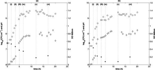
Cells which were subjected to an acid stress at pH 3.3 were removed at the six following characteristic phases of growth (Fig. 1): (i) beginning of the exponential phase (1.67 h after inoculation; optical density at 600 nm [OD₆₀₀] for L. monocytogenes, 0.10; OD₆₀₀ for S. enterica serovar Typhimurium, 0.15); (ii) middle of the exponential phase (3.33 h after inoculation; OD₆₀₀ for L. monocytogenes, 0.20; OD₆₀₀ for S. enterica serovar Typhimurium, 0.60); (iii) end of the exponential phase (5 h after inoculation; OD₆₀₀ for L. monocytogenes, 0.55; OD₆₀₀ for S. enterica serovar Typhimurium, 0.70); (iv) deceleration phase (6.67 h after inoculation; OD₆₀₀ for L. monocytogenes, 0.70; OD₆₀₀ for S. enterica serovar Typhimurium, 0.75); (v) early stationary phase (12 h after inoculation; OD₆₀₀ for L. monocytogenes, 0.80; OD₆₀₀ for S. enterica serovar Typhimurium, 0.85); and (vi) late stationary phase (17 h after inoculation; OD₆₀₀ for L. monocytogenes, 0.85; OD₆₀₀ for S. enterica serovar Typhimurium, 0.80).

FIG. 1.

Evolution of the population size (○) (CFU ml⁻¹), the optical density at 600 nm (DO 600nm) (⋄), and the pH (*) during growth preceding inactivation of L. monocytogenes (a) and S. enterica serovar Typhimurium (b). The characteristic phases of growth are the beginning of the exponential phase (i), the middle of the exponential phase (ii), the end of the exponential phase (iii), deceleration of the exponential phase (iv), the early stationary phase (v), and the late stationary phase (vi).

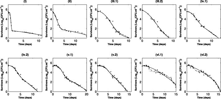
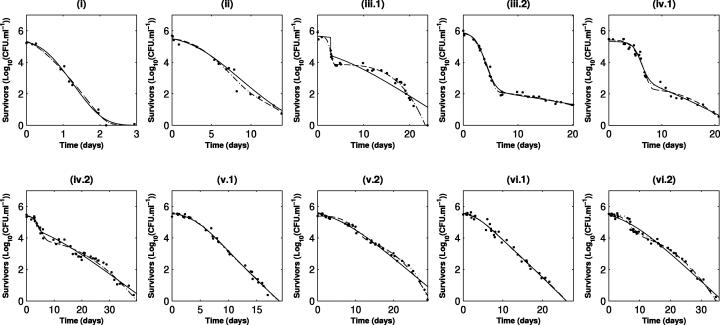
The survival curves for S. enterica serovar Typhimurium show continuous and progressive evolution from a biphasic shape to a simple concave shape whether cells were taken from early or late stages of growth (Fig. 2). This evolution seems to correspond to the gradual disappearance of a sensitive subpopulation. In the case of L. monocytogenes (Fig. 3), the initial presence of two subpopulations is less clear, but a drastic increase in the general resistance of bacteria is observed; while elimination of the total population seems to occur within around 3 days for cells in the early stage of growth (Fig. 3, panels i), it takes more than 30 days before the same level of inactivation is reached when cells are removed at the late stationary phase (Fig. 3, panels vi).

FIG. 2.

Evolution of the shape of survival curves for S. enterica serovar Typhimurium and fitted curves for the models. Solid line, Whiting's model (model 1); dotted line, model 2; dashed line, simplified model 3. The data obtained are indicated by symbols. i, ii, iii, iv, v, and vi indicate the characteristic phases of growth from which the inocula used for inactivation kinetics analysis were obtained (see the legend to Fig. 1); 1 and 2 indicate repetitions.

FIG. 3.

Evolution of the shape of survival curves for L. monocytogenes and fitted curves for the models. Solid line, Whiting's model (model 1); dotted line, model 2; dashed line, simplified model 3. The data obtained are indicated by symbols. i, ii, iii, iv, v, and vi indicate the characteristic phases of growth from which the inocula used for inactivation kinetics analysis were obtained (see the legend to Fig. 1); 1 and 2 indicate repetitions.

Quality of fit.

We compared Whiting's model (model 1) and the two new proposed models for describing the survival of bacteria at various times during incubation of subcultures (Fig. 2 and 3).

Model 2, which includes one more parameter than the other models, provided, as expected, the best fit for the data according to the minimum sum of squares[C(θ)] for 16 of 20 curves observed (Table 1). However, this model was the worst model according to the AIC, which takes both the fit and parsimony into account. In most cases, Whiting's model (model 1) and the simplified model (model 3) showed quite similar results for goodness of fit according to the AIC. The double Weibull simplified model (model 3) showed a slight tendency for better fit with 14 smaller AIC for the 20 kinetics observed. In some cases, there were great differences between the two AIC in favor of model 3 (Table 1; Fig. 2, panels vi; Fig. 3, panels iii and vi). In these cases model 3 provided a very small AIC value compared to the value for model 1; the difference could be as high as about 20 U for Salmonella and 70 U for Listeria.

TABLE 1.

Minimum C(θ) and AIC values for the different survival curves of S. enterica serovar Typhimurium and L. monocytogenes^a

Organism	Culture phase	Repetition	Length of incubation of subculture (min)	n	C(θ)			SL	AIC
					Model 1	Model 2	Model 3		Model 1	Model 2	Model 3
S. enterica serovar	Beginning of exponential	1	100	13	0.119	0.082	0.089	0.92	−14.11	−16.85	−17.93
Typhimurium	Mid-exponential	1	200	16	0.742	0.677	0.751	1.65	6.31	6.84	6.49
	End of exponential	1	300	19	1.796	1.602	1.602	0.00	19.13	18.96	16.96
		2	300	20	1.131	0.984	1.027	0.03	11.33	9.38	7.41
	Deceleration of exponential	1	400	24	1.054	1.069	1.115	1.00	3.12	5.45	4.46
		2	400	22	0.822	0.784	0.784	0.02	2.14	1.09	−0.90
	Early stationary	1	720	38	0.825	0.772	0.874	4.73	−27.67	−28.22	−25.49
		2	720	33	1.246	1.039	1.108	2.11	−2.48	−8.44	−8.33
	Late stationary	1	1,020	31	2.067	1.018	1.122	3.00	14.04	−5.91	−4.91
		2	1,020	34	1.510	1.085	1.085	0.00	2.61	−8.62	−10.62
L. monocytogenes	Beginning of exponential	1	100	11	0.452	0.455	0.460	0.14	6.15	8.22	6.35
	Mid-exponential	1	200	16	1.076	1.045	1.046	0.01	12.25	13.78	11.79
	End of exponential	1	300	33	7.618	0.887	0.887	0.01	55.29	−13.69	−15.69
		2	300	29	0.689	0.549	0.552	6.58	−14.13	−20.70	−22.54
	Deceleration of exponential	1	400	30	1.452	1.196	1.444	5.65	4.31	0.48	4.13
		2	400	48	3.244	2.324	2.326	0.03	18.90	2.89	0.92
	Early stationary	1	720	32	0.560	0.542	0.571	1.72	−28.65	−27.70	−27.99
		2	720	41	1.592	0.361	0.591	20.15	−4.84	−65.63	−47.48
	Late stationary	1	1,020	36	1.069	1.057	1.059	0.04	−14.44	−12.82	−14.78
		2	1,020	46	2.655	0.812	0.935	6.50	9.35	−43.17	−38.67

^aThe S_L values are related to the simplification of model 2 used to obtain model 3; boldface S_L values represent rejection of the simplification. Boldface C(θ) and AIC values are the best C(θ) and AIC values.

It was also noted that the confidence intervals related to Whiting's model (model 1) were larger, especially for the f value (results not shown). The confidence intervals of the estimated parameters and the AIC of model 3 were smaller, showing that there was better estimation of parameters and a better compromise between the goodness of fit and the parsimony.

The hypothesis that there was equality between p₁ and p₂ of model 2 was at the origin of model 3. If the likelihood ratio test value (S_L) is lower than the value of χ² with 1 degree of freedom for a significance level of 0.05, the hypothesis tested cannot be rejected. The hypothesis was not rejected by the likelihood ratio test in 15 of 20 cases (Table 1). One of the two repetitions was not validated for cases iii to vi of L. monocytogenes (Fig. 3). The AIC was favorable for simplification of the double Weibull model. This simplification allowed removal of one parameter while nearly the same goodness of fit was kept.

Effect of the physiological state on the estimated parameters of models.

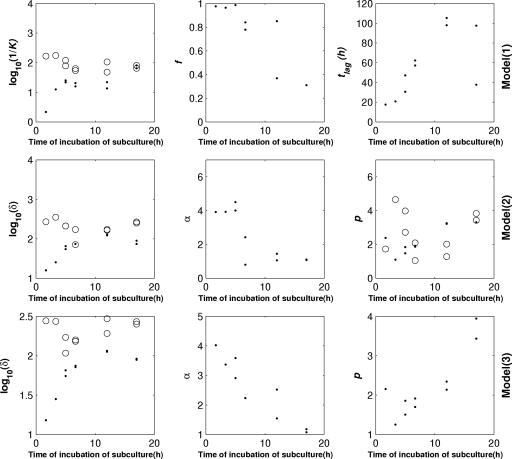
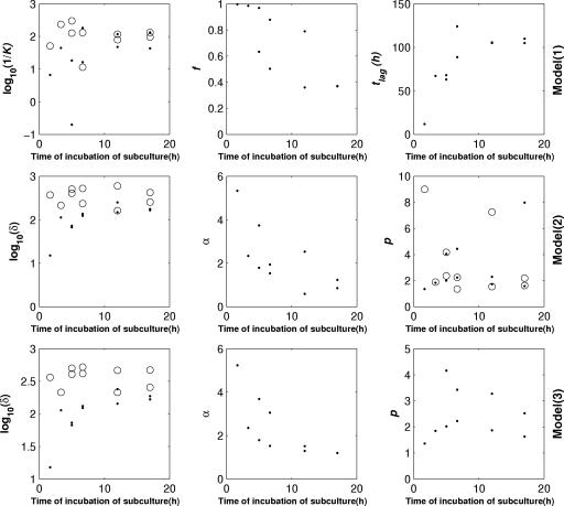
According to Whiting's model (model 1) for the two species studied, the estimated f ratio decreased from 100% to 30% after 300 min of incubation of the subculture, while the estimated t_lag values increased from an average of 15 h to more than 100 h and then seemed to stabilize at an average of 720 min (model 1) (Fig. 4 and 5). For Salmonella, the estimated t_lag values were very different for the last two replicates, but the associated confidence intervals were wide. For the two species studied, the k₁ value fell to a value close to the k₂ value, which was approximately constant (average, 0.01 h⁻¹).

FIG. 4.

Evolution of the estimated parameters versus time of incubation of the subculture for S. enterica serovar Typhimurium for Whiting's model (model 1), the double Weibull model (model 2), and the double Weibull simplified model (model 3). •, k₁, f, t_lag, δ₁, α, p, and p₁ values; ○, k₂, δ₂, and p₂ values.

FIG. 5.

Evolution of the estimated parameters versus the time of incubation of the subculture for L. monocytogenes for Whiting's model (model 1), the double Weibull model (model 2), and the double Weibull simplified model (model 3). •, k₁, f, t_lag, δ₁, α, p, and p₁ values; ○, k₂, δ₂, and p₂ values.

The estimated δ₂ values of model 2 did not seem to change with the duration of incubation of the subculture; for Salmonella, this value was close to 200 h. For the two species, the δ₁ values increased from 15 h to more than 100 h and tended toward the δ₂ values. The values of α decreased from 4 and 5 for Salmonella and Listeria, respectively, to 1, equivalent to f values of 99.990%, 99.999%, and 90.909%, respectively. However, the profiles of the evolution of the parameters were quite different. For Salmonella, the value of α was 4 for incubation of the subculture for less than 300 min; after this the α value decreased to 1. In contrast to the α value for Salmonella, which decreased quickly from 5.3 to 2 for incubation less than 400 min long, for Listeria the α value continued to decrease slowly to 1 after this time. The p₁ and p₂ values were very variable and were between 1 and 31.

With the double Weibull simplified model (model 3), the changes in the δ parameters were similar to the changes observed with model 2. The only differences in behavior between these two models concerned the α and p parameters. Compared to model 2, the rate of decrease of estimated α values for model 3 was less variable for the two species. The p value was relatively stable except for cells from the late stationary phase, for which the value had a slight tendency to increase for Salmonella. The median of the p value was close to 2 for the two species.

DISCUSSION

As expected, the resistance of bacterial populations to stress increased as the stationary phase approached. Such an increase in the resistance of cultures results from the initiation of mechanisms depending on physicochemical factors of the bacterial environment and also on the reduction in the metabolic activity of cells (4, 25, 33, 42). A clear change in shape of the inactivation kinetic curves was noted.

The evolution of the parameter values related to models was directly linked to the increase in the resistance. The inactivation rate (k₁) or the first decimal reduction time (δ₁) of the more sensitive population increased, while the rate of inactivation of the resistant population was unchanged over a wide range. The decrease in the f ratio, or its logit α, corresponding to an increase in the ratio for the more resistant cells, occurred at the beginning of this change. Whiting's model had five parameters, four of which (k₁, k₂, f, and t_lag) characterize the evolution of the resistance of the overall population with respect to the duration of incubation of the subculture. On the other hand, the double Weibull simplified model (model 3) also had five parameters, but only three of these parameters (δ₁, δ₂, and α) were related to the physiological state of the cells and environmental conditions.

Furthermore, models 1 and 3 presented equivalent qualities of fit except for f for Salmonella (Fig. 2 and Table 1) and f and c for Listeria (Fig. 3 and Table 1). In these cases, the shape of the kinetics was biphasic nonlinear. Whiting's model is based on a linear decrease in the size of the subpopulation after latency to mortality. It was unable to describe the concave decrease observed in these cases, which explains the bad AIC value related to Whiting's model (model 1). The double Weibull simplified model (model 3) is more flexible and could describe the biphasic nonlinear shape (p greater than 1), as well as the biphasic linear case (p equal to 1).

With narrower confidence intervals, the double Weibull model described the adaptation of cells better than the model of Whiting. For the first four periods of incubation corresponding to the exponential phase of a subculture, the time necessary for the first decimal reduction (δ₁) value increased and stabilized at the δ₂ value during the stationary growth phase of the subculture (Fig. 4 and 5). This change indicated that there was adaptation of the cells from the more sensitive subpopulation, subpopulation 1, whose level of resistance to stress tended gradually toward the level of resistance of subpopulation 2. The resistance of subpopulation 2 was stable. The α value decreased as the subculture progressed through various stages of growth, indicating the increase in the ratio of the subpopulation resistant to stress. The increase in the resistance to stress was described well by the combined changes in all parameters, which indicated the progressive change in resistance from sensitive to resistant. Subpopulation 1 assumed by the model was the more sensitive subpopulation and did not activate or slightly activated the mechanisms of resistance. Subpopulation 2 corresponded to the most resistant cells which had restricted metabolic activity and developed the mechanisms of resistance. When the resistance is minimal and when the resistance is maximal, a single population should be observed, corresponding to subpopulations 1 and 2, respectively. Then the resistance to stress should follow a simple Weibull distribution.

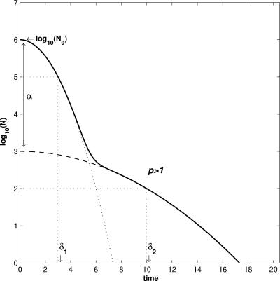
One advantage of the parameterization and simplification of model 3 is that all parameters can be graphically interpreted (Fig. 6), as follows: N₀ is the initial size of the population; δ is the time of the first logarithm decline for the two subpopulations; α is defined as the logit of f and is equivalent to α = log₁₀(N₀₁/N₀₂), and the α value then is close to the graphic difference between log₁₀(N₀) and the logarithm of the population size where the inflection is observed; and p represents the shape of the curve (see below).

FIG. 6.

Diagram of survival model based on the double Weibull distribution of resistance. Solid line, microbial population; dotted line, subpopulation 1; dashed line, subpopulation 2. Subpopulation 1 represented bacteria that were more sensitive to the stress, and subpopulation 2 represented the cells that were more resistant.

In theory, the α value can be equal to all real numbers. In practice, no inflection point can be obviously observed graphically for a negative α value. This is also the case if the value is higher than the difference between log₁₀(N₀) and the decimal logarithm of the detection limit of the technique used for enumeration. In this case, the α value is not observed and cannot be estimated.

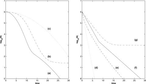
The double Weibull simplified model allows workers to fit most of the shapes of inactivation curves (Fig. 7). With two populations, it can describe, in the general case, a biphasic shape with a nonlinear decrease (Fig. 7, curve a). Note that this shape cannot be described by the other models used in bacterial inactivation studies with constant stress conditions. The model can also describe a sigmoidal shape (curve b) if δ₂ tends toward infinity, a biphasic shape (curve f) if p is equal to 1, and a linear shape with a tail (curve g) if δ₂ tends toward infinity and p is equal to 1.

FIG. 7.

Different shapes of inactivation curves, including biphasic with a nonlinear decrease (curve a), sigmoidal (curve b), concave (curve c), linear (curve d), convex (curve e), biphasic (curve f), and linear with a tail (curve g).

Simplification of the double Weibull model to a simple model can be obtained by using a negative value of α or α > log₁₀(N₀/detection limit) or equality between the two δ values. Then the model permits fitting of a linear shape (curve d) if p is equal to 1, a concave shape (curve c) if p is >1, and a convex shape (curve e) if p is <1.

Further research is required to allow use of the double Weibull model in nonthermal inactivation studies. The evolution of p depending on environmental factors and the physiological state of the cells requires special attention. In some cases of thermal treatment, it can be considered constant (15, 16, 35, 44). The advantage of the Weibull model is that it has great flexibility because of a strong correlation between the scale (δ) and the shape (p) parameters. If the p value is estimated to be constant for different stress conditions, the δ parameter is able to balance this constraint to give a good quality of fit of the model for the data. If this phenomenon could be confirmed in nonthermal inactivation studies, the double Weibull model might be a convenient model for describing the kinetics as a function of the physiological state of the cells and the stress conditions with only three parameters. Indeed, the δ parameters might change according to the intensity of stress, and the δ₁ and α parameters might change according to the physiological state of the treated cells, as shown here.

REFERENCES

- 1.Akaike, H. 1973. Information theory and extension of the maximum likelihood principle, p. 267-281. In B. N. Petrov and and F. Cza'ki (ed.). Proceedings of the 2nd International Symposium of Information Theory. Akademiai Kiado, Budapest, Hungary.
- 2.Albert, I., and P. Mafart. 2005. A modified Weibull model for bacterial inactivation. Int. J. Food Microbiol. 100:197. [DOI] [PubMed] [Google Scholar]
- 3.Baranyi, J., and T. A. Roberts. 1994. A dynamic approach to predicting bacterial growth in food. Int. J. Food Microbiol. 23:277. [DOI] [PubMed] [Google Scholar]
- 4.Booth, I. R. 2002. Stress and the single cell: intrapopulation diversity is a mechanism to ensure survival upon exposure to stress. Int. J. Food Microbiol. 78:19. [DOI] [PubMed] [Google Scholar]
- 5.Breand, S. 1998. Etude biométrique de la réponse d'une population bactérienne à une variation défavorable de température ou de pH. Université Claude Bernard, Lyon, France.
- 6.Buchanan, R. L., M. A. Golden, R. C. Whiting, J. G. Phillips, and J. L. Smith. 1994. Non-thermal inactivation models for Listeria monocytogenes. J. Food Sci. 59:179-188. [Google Scholar]
- 7.Buchanan, R. L., and M. H. Golden. 1994. Interaction of citric acid concentration and pH on the kinetics of Listeria monocytogenes inactivation. J. Food Prot. 57:567-570. [DOI] [PubMed] [Google Scholar]
- 8.Buchanan, R. L., and M. H. Golden. 1998. Interactions between pH and malic acid concentration on the inactivation of Listeria monocytogenes. J. Food Saf. 18:37-48. [Google Scholar]
- 9.Buchanan, R. L., M. H. Golden, and J. G. Phillips. 1997. Expanded models for the non-thermal inactivation of Listeria monocytogenes. J. Appl. Microbiol. 82:567-577. [DOI] [PubMed] [Google Scholar]
- 10.Buchanan, R. L., M. H. Golden, and R. C. Whiting. 1993. Differentiation of the effects of pH and lactic or acetic acid concentration on the kinetics of Listeria monocytogenes inactivation. J. Food Prot. 56:474-478. [DOI] [PubMed] [Google Scholar]
- 11.Reference deleted.
- 12.Cerf, O. 1977. Tailing of survival curves of bacterial spores, a review. J. Appl. Bacteriol. 42:1-19. [DOI] [PubMed] [Google Scholar]
- 13.Cole, M. B., K. W. Davies, G. Munro, C. D. Holyoak, and D. C. Kilsby. 1993. A vitalistic model to describe the thermal inactivation of Listeria monocytogenes. J. Ind. Microbiol. 12:232-239. [Google Scholar]
- 14.Corradini, M. G., and M. Peleg. 2003. A model of microbial survival curves in water treated with a volatile disinfectant. J. Appl. Microbiol. 95:1268-1276. [DOI] [PubMed] [Google Scholar]
- 15.Couvert, O., S. Gaillard, N. Savy, P. Mafart, and I. Leguerinel. 2005. Survival curves of heated bacterial spores: effect of environmental factors on Weibull parameters. Int. J. Food Microbiol. 101:73. [DOI] [PubMed] [Google Scholar]
- 16.Fernandez, A., J. Collado, L. M. Cunha, M. J. Ocio, and A. Martinez. 2002. Empirical model building based on Weibull distribution to describe the joint effect of pH and temperature on the thermal resistance of Bacillus cereus in vegetable substrate. Int. J. Food Microbiol. 77:147-153. [DOI] [PubMed] [Google Scholar]
- 17.Geeraerd, A. H., C. H. Herremans, and J. F. Van Impe. 2000. Structural model requirements to describe microbial inactivation during a mild heat treatment. Int. J. Food Microbiol. 59:185-209. [DOI] [PubMed] [Google Scholar]
- 18.Greenacre, E. J., T. F. Brocklehurst, C. R. Waspe, D. R. Wilson, and P. D. G. Wilson. 2003. Salmonella enterica serovar Typhimurium and Listeria monocytogenes acid tolerance response induced by organic acids at 20°C: optimization and modeling. Appl. Environ. Microbiol. 69:3945-3951. [DOI] [PMC free article] [PubMed] [Google Scholar]
- 19.Hajmeer, M., I. Basheer, C. Hew, and D. O. Cliver. 2006. Modeling the survival of Salmonella spp. in chorizos. Int. J. Food Microbiol. 107:59-67. [DOI] [PubMed] [Google Scholar]
- 20.Huet, S., A. Bouvier, M. A. Gruet, and E. Jolivet. 2003. Statistical tools for nonlinear regression. A practical guide with S-PLUS examples. Springer-Verlag, New York, NY.
- 21.Janssen, M., A. H. Geeraerd, A. Cappuyns, L. Garcia-Gonzalez, K. M. Vereecken, F. Devlieghere, and J. F. Van Impe. 2005. Presented at the III International Symposium on Applications of Modelling as an Innovative Technology in the Agri-Food Chain, MODEL-IT, Leuven, Belgium.
- 22.Janssen, M., K. M. Vereecken, A. H. Geeraerd, A. Cappuyns, and J. F. Van Impe. 2004. Presented at the International Congress on Engineering and Food, Montpellier, France.
- 23.Kamau, D. N., S. Doores, and K. M. Pruitt. 1990. Enhanced thermal destruction of Listeria monocytogenes and Staphylococcus aureus by the lactoperoxidase system. Appl. Environ. Microbiol. 56:2711-2716. [DOI] [PMC free article] [PubMed] [Google Scholar]
- 24.Koutsoumanis, K., K. Lambropoulou, and G. E. Nychas. 1999. A predictive model for the non-thermal inactivation of Salmonella enteritidis in a food model system supplemented with a natural antimicrobial. Int. J. Food Microbiol. 49:63-74. [DOI] [PubMed] [Google Scholar]
- 25.Lee, I. S., J. L. Slonczewski, and J. W. Foster. 1994. A low-pH-inducible, stationary-phase acid tolerance response in Salmonella typhimurium. J. Bacteriol. 176:1422-1426. [DOI] [PMC free article] [PubMed] [Google Scholar]
- 26.Leroy, F., and L. de Vuyst. 1999. Temperature and pH conditions that prevail during fermentation of sausages are optimal for production of the antilisterial bacteriocin sakacin K. Appl. Environ. Microbiol. 65:974-981. [DOI] [PMC free article] [PubMed] [Google Scholar]
- 27.Leroy, F., K. Lievens, and L. De Vuyst. 2005. Modeling bacteriocin resistance and inactivation of Listeria innocua LMG 13568 by Lactobacillus sakei CTC 494 under sausage fermentation conditions. Appl. Environ. Microbiol. 71:7567-7570. [DOI] [PMC free article] [PubMed] [Google Scholar]
- 28.Little, C. L., M. R. Adams, W. A. Anderson, and M. B. Cole. 1994. Application of a log-logistic model to describe the survival of Yersinia enterocolitica at sub-optimal pH and temperature. Int. J. Food Microbiol. 22:63-71. [DOI] [PubMed] [Google Scholar]
- 29.Mafart, P., O. Couvert, S. Gaillard, and I. Leguerinel. 2002. On calculating sterility in thermal preservation methods: application of Weilbull frequency distribution model. Int. J. Food Microbiol. 72:107-113. [DOI] [PubMed] [Google Scholar]
- 30.McQuarrie, A. D., and C.-L. Tsai. 1998. Regression and time series model selection. World Scientific Publishing, River Edge, N.J.
- 31.Membre, J. M., V. Majchrzac, and I. Jolly. 1997. Effects of temperature, pH, glucose and citric acid on the inactivation of Salmonella typhimurium in reduced calorie mayonnaise. J. Food Prot. 60:1497-1501. [DOI] [PubMed] [Google Scholar]
- 32.Membre, J. M., J. Thurette, and M. Catteau. 1997. Modelling the growth, survival and death of Listeria monocytogenes. J. Appl. Microbiol. 82:345-350. [DOI] [PubMed] [Google Scholar]
- 33.O'Driscoll, B., C. Gahan, and C. Hill. 1996. Adaptive acid tolerance response in Listeria monocytogenes: isolation of an acid-tolerant mutant which demonstrates increased virulence. Appl. Environ. Microbiol. 62:1693-1698. [DOI] [PMC free article] [PubMed] [Google Scholar]
- 34.Peleg, M., and M. B. Cole. 1998. Reinterpretation of microbial survival curves. Crit. Rev. Food Sci. Nutr. 38:353. [DOI] [PubMed] [Google Scholar]
- 35.Peleg, M., and C. M. Penchina. 2000. Modelling microbial survival during exposure to a lethal agent with varying intensity. Crit. Rev. Food Sci. Nutr. 40:159-172. [DOI] [PubMed] [Google Scholar]
- 36.Phan-Thanh, L., F. Mahouin, and S. Alige. 2000. Acid responses of Listeria monocytogenes. Int. J. Food Microbiol. 55:121-126. [DOI] [PubMed] [Google Scholar]
- 37.Ross, E. W., I. A. Taub, C. J. Doona, F. E. Feeherry, and K. Kustin. 2005. The mathematical properties of the quasi-chemical model for microorganism growth-death kinetics in foods. Int. J. Food Microbiol. 99:157. [DOI] [PubMed] [Google Scholar]
- 38.Samelis, J., J. N. Sofos, P. A. Kendall, and G. C. Smith. 2001. Influence of the natural microbial flora on the acid tolerance response of Listeria monocytogenes in a model system of fresh meat decontamination fluids. Appl. Environ. Microbiol. 67:2410-2420. [DOI] [PMC free article] [PubMed] [Google Scholar]
- 39.Skandamis, P. N., K. W. Davies, P. J. McClure, K. Koutsoumanis, and T. Tassou. 2002. A vitalistic approach for non-thermal inactivation of pathogens in traditional Greek salads. Food Microbiol. 19:405-421. [Google Scholar]
- 40.Skandamis, P. N., and G. E. Nychas. 2003. Modeling the microbial interaction and the death of Escherichia coli O157:H7 during the fermentation of Spanish-style green table olives. J. Food Prot. 66:1166-1175. [DOI] [PubMed] [Google Scholar]
- 41.Takumi, K., R. De Jonge, and A. Havelaar. 2000. Modelling inactivation of Escherichia coli by low pH: application to passage through the stomach of young and elderly people. J. Appl. Microbiol. 89:935-943. [DOI] [PubMed] [Google Scholar]
- 42.Testerman, T. L., A. Vazquez-Torres, Y. Xu, J. Jones-Carson, S. J. Libby, and F. C. Fang. 2002. The alternative sigma factor sigmaE controls antioxidant defences required for Salmonella virulence and stationary-phase survival. Mol. Microbiol. 43:771-782. [DOI] [PubMed] [Google Scholar]
- 43.Valdramidis, V. P., A. H. Geeraerd, K. Bernaerts, F. Devlieghere, J. Debevere, and J. F. Van Impe. 2004. Accurate modelling of non-loglinear survival curves. Bull. Int. Dairy Fed. 392:97-110. [Google Scholar]
- 44.van Boekel, M. A. J. S. 2002. On the use of the Weibull model to describe thermal inactivation of microbial vegetative cells. Int. J. Food Microbiol. 74:139. [DOI] [PubMed] [Google Scholar]
- 45.Virto, R., D. Sanz, I. Alvarez, Condon, and J. Raso. 2005. Inactivation kinetics of Yersinia enterocolitica by citric and lactic acid at different temperatures. Int. J. Food Microbiol. 103:251. [DOI] [PubMed] [Google Scholar]
- 46.Whiting, R. C. 1995. Microbial modeling in foods. Crit. Rev. Food Sci. Nutr. 35:467-494. [PubMed] [Google Scholar]
- 47.Whiting, R. C. 1993. Modeling bacterial survival in unfavorable environments. J. Ind. Microbiol. 12:240-246. [Google Scholar]
- 48.Whiting, R. C., S. Sackitey, S. Calderone, K. Morely, and J. G. Phillips. 1996. Model for the survival of Staphylococcus aureus in nongrowth environments. Int. J. Food Microbiol. 31:231-243. [DOI] [PubMed] [Google Scholar]
- 49.Xiong, R., G. Xie, A. E. Edmondson, and M. A. Sheard. 1999. A mathematical model for bacterial inactivation. Int. J. Food Microbiol. 46:45-55. [DOI] [PubMed] [Google Scholar]