Predicting protein–protein interaction by searching evolutionary tree automorphism space

Abstract

Motivation

Uncovering the protein–protein interaction network is a fundamental step in the quest to understand the molecular machinery of a cell. This motivates the search for efficient computational methods for predicting such interactions. Among the available predictors are those that are based on the co-evolution hypothesis “evolutionary trees of protein families (that are known to interact) are expected to have similar topologies”. Many of these methods are limited by the fact that they can handle only a small number of protein sequences. Also, details on evolutionary tree topology are missing as they use similarity matrices in lieu of the trees.

Results

We introduce MORPH, a new algorithm for predicting protein interaction partners between members of two protein families that are known to interact. Our approach can also be seen as a new method for searching the best superposition of the corresponding evolutionary trees based on tree automorphism group. We discuss relevant facts related to the predictability of protein–protein interaction based on their co-evolution. When compared with related computational approaches, our method reduces the search space by ~3 × 10⁵-fold and at the same time increases the accuracy of predicting correct binding partners.

1 INTRODUCTION

Protein–protein interactions are of primary importance in metabolic and signaling pathways. Traditional experimental techniques (genetic, biochemical or biophysical) for the study of individual interactions have been followed by high-throughput interaction-detection methods such as two-hybrid systems, and protein complex purification using mass spectrometry. Several computational approaches for predicting interactions have also been developed. Methods based on genomic information such as phylogenetic profiling (Huynen and Bork, 1998; Pellegrini et al., 1999), gene order conservation (Dandekar et al., 1998; Overbeek et al., 1998) and gene fusion (Marcotte et al., 1999) have been successfully applied to predict sets of functionally related proteins. Sequence-based methods include the study of correlated mutations (Pazos and Valencia, 2002) and similarity of phylogenetic trees (Goh et al., 2000; Goh and Cohen, 2002; Pazos et al., 1997; Pazos and Valencia, 2001; Ramani and Marcotte, 2003). The underlying assumption of the latter is that proteins and their interaction partners must co-evolve so that divergent changes in one partner’s binding surface are complemented in the interface with the other partner. This could explain the fact that phylogenetic trees of ligands show significant similarity to the corresponding trees of receptors.

The co-evolution of interacting partners can be used to predict protein–protein interaction. One approach is to take two families of orthologous interacting proteins such that each family contains proteins from the same set of species. The level of co-evolution between the two families can be tested by assessing the agreement between the corresponding similarity matrices (Pazos and Valencia, 2001, 2002; Valencia and Pazos, 2003). The agreement between two trees is usually calculated using some information-theoretic similarity agreement measure (usually correlation coefficient) of the corresponding similarity matrices. A significant correlation between the evolutionary trees indicates that the proteins from the two families may interact. Pazos and Valencia observed that this “mirror tree” approach can be used as a predictor of protein interaction with >66% of true positives at correlation coefficient values better than 0.8 on a −1.0 to +1.0 scale.

Correlation of phylogenetic trees can also be used to predict specific interaction partners between members of two families that are known to interact. Assume that each protein in one family interacts with exactly one protein in the other family. In this case we have two similar (by the assumption of co-evolution) phylogenetic trees and the objective is to establish a mapping between the leaves of the two trees resulting in a one-to-one mapping between the members of one family and those of the other (Ramani and Marcotte, 2003; Gertz et al., 2003). The idea is to identify the mapping that “maximizes” the correlation between the two similarity matrices. However, this is computationally intensive. The number of possible mappings between two n × n matrices is equal to n!, a function that grows faster than any exponential function. Ramani and Marcotte, and Gertz et al. independently proposed a Monte Carlo algorithm that explores the search space of all possible superpositions of two similarity matrices. In a single Monte Carlo step, the algorithm picks a pair of columns uniformly at random and tests how swapping these columns (and the corresponding rows) would affect the score (e.g. correlation coefficient) of the matrix superposition. The swap is subsequently accepted/rejected using the Metropolis criterion (Metropolis et al., 1953). Ramani and Marcotte observed that such an algorithm cannot address the problem successfully if the size of the matrices is large (>30) or if the evolutionary trees are not sufficiently “complex”. The obstacle to a successful prediction is the large search space, large number of possible moves at each iteration and the possibility of getting trapped in a local optimum.

In this paper we propose a new algorithm called MORPH to detect interacting pairs based on the co-evolution hypothesis. The main idea in our approach is to reduce the search space and the move-set by using information encoded in the evolutionary trees of the two families. In other words, in addition to using the evolutionary distance information, we use the topological information of the evolutionary trees. As a result, our reduced move-set greatly minimizes the chances of getting trapped in a local optimum. We also introduce the concept of entropy of an evolutionary tree and the information content of such a tree. We argue that these concepts provide a formal measure of complexity of a tree, similar to that discussed informally by Ramani and Marcotte.

We present a few graph-theoretic terms before introducing our approach. We call two trees (graphs in general) isomorphic if there is a one-to-one mapping between their vertices (nodes) such that there is an edge between two vertices of one graph if and only if there is an edge between the two corresponding vertices in the other graph. Graph automorphism is an isomorphism of a graph to itself. A graph can have more than one automorphism.

Similarly to the previous algorithms mentioned above, MORPH is based on a Monte Carlo search. However, the search space and the method of searching are different. In our approach, the search space corresponds to the automorphism group of a phylogenetic tree (after some preprocessing), and each move corresponds to an automorphism of the tree onto itself. In the extreme case, where the information content of the evolutionary tree is zero, our search space becomes as big as the search space explored by the algorithms of Ramani and Marcotte and Gertz et al. However, if the evolutionary tree carries some information (which is usually the case), MORPH is able to use this information to reduce the search space drastically.

2 CO-EVOLUTION, TREE AUTOMORPHISMS AND TREE COMPLEXITY

To illustrate the intuition behind our method, let us first consider an ideal case. Assume that the evolutionary trees for both families (that are known to interact) have identical topologies (they are isomorphic). Furthermore, assume that all edges have high bootstrap values,¹ thus the trees are reliable. We only need to focus on topology-preserving embeddings of one tree onto the other tree, where by a topology-preserving embedding we mean an isomorphic mapping of the two trees.

For illustration, consider the three pairs of trees given in Figure 1. We use the term cherry to denote any subtree of a tree that consists of one internal node and a set of leaves. In Figure 1(a), there are eight possible topology preserving superpositions of the two trees: any “cherry”, say (a, b), of the bottom tree can be superimposed with any cherry (A, B) or (C, D) of the top tree and within each cherry any of the two leaf mappings are possible. The number of superpositions of the pair of trees in Figure 1(b) is also eight, despite the fact they have one additional leaf compared with the trees in Figure 1(a). This is because the middle leaf, e, of the bottom tree can be mapped only to the middle leaf, E, of the top tree (or else the topology will not be preserved). Finally, the pair in Figure 1(c) has one fewer leaves compared to the trees in Figure 1(b) but has the largest possible number of superpositions (4! = 24) among the three pairs in Figure 1. In this case any leaf of one tree can be mapped to any leaf of the other tree without violating the tree topology. Here the topology of the evolutionary tree does not provide any additional information that would be helpful in reducing the number of possible mappings.

Fig. 1.

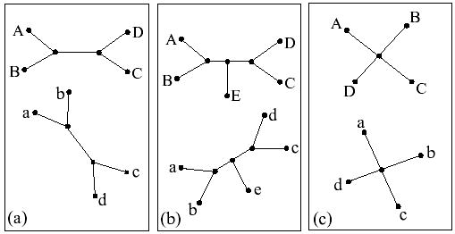
Three pairs of isomorphic (topologically identical) trees. The number of topology-preserving superpositions of one tree onto another is (a) 8, (b) 8 and (c) 24.

If two trees are isomorphic, the number of topology-preserving mappings between the two trees will be same as the number of topology-preserving mappings of one of those trees onto itself. In other words, when two trees are isomorphic, the total number of mappings between those trees is the same as the number of automorphisms of either of those two trees. Let τ (T) denote the number of automorphisms of tree T. We define the topological entropy E_N (T) of a tree T with N leaf nodes to be

$$E_N(T)=log\tau (T).$$

Consistent with the information-theoretic definition, we define the information content I (T) of a tree T to be

$$I(T)=log(N!)-E_N(T).$$

The tree with the highest entropy among all trees with N leaf nodes is the star tree (see Fig. 1c for a star tree with N = 4). The entropy of a star tree is log (N!) ~ N log N. Thus, the information content of any star tree is zero (regardless of the tree size).

Information content measures the reduction in the search space achieved by our approach. In fact, the ratio of the size of the search space (number of all possible permutations) used by the previous algorithms to the size of the search space (number of tree automorphisms) used by MORPH is equal to 2^{I (T)}. As an example, consider the pair of nine-node trees in Figure 2(a). The search space of a column-flipping algorithm for this pair of trees is 9! = 362,880 while the size of the automorphism space is only 1,296. The information content for this set of trees is >2 bits and the reduction in search space is 280-fold.

Fig. 2.

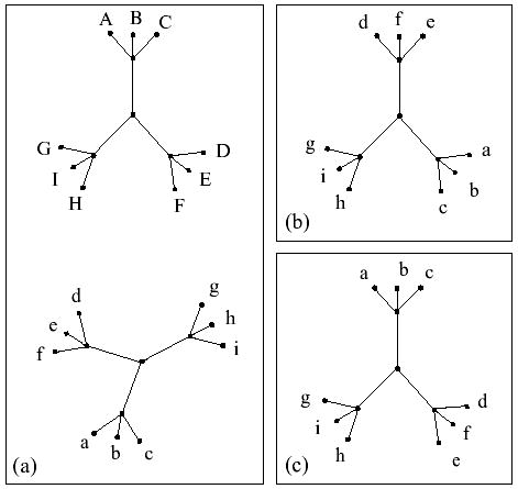
(a) A pair of highly symmetrical trees. The search space size of the column-swapping approach for this pair of trees is 9! = 362 880, and the automorphism space has size (3!)⁴ = 1296. (b) and (c) two possible topology-preserving superpositions of the lower tree in (a). MORPH can move between (b) and (c) in one step. The column swapping approach is highly likely to get stuck in the local minimum represented in Figure 1b.

The entropy E_N (T) of a tree measures precisely how symmetric a tree T with N leaf nodes is and therefore provides a formal measure of tree ‘complexity’. The smaller the E_N (T), the more complex the tree T is. Based on the entropy of the similarity matrix, Ramani and Marcotte (2003) proposed a different method for measuring the complexity of a tree. Their idea is to bin the numerical entries of the similarity matrix M, and compute H(M) of the distribution of M’s entries:

$$H(M)=-\sum _{x}p(x)logp(x),$$

where x represents the bins of values and p(x) is the frequency with which those values are seen in the matrix. The intuition behind their approach is that the larger the number of unique (non-identical) entries/values in the matrix, the more complex the tree obtained from that matrix would be. The authors suggest that H(M) is larger for more complex trees. Clearly H(M) is minimized when all entries are equal (which corresponds to a least-complex star tree). Unfortunately, H(M), in general, does not need to increase monotonically with the complexity of a tree. Note, for example, that in Figure 3, the first tree is more complex than the second despite the fact that the similarity matrix of the first tree has significantly smaller entropy.

Fig. 3.

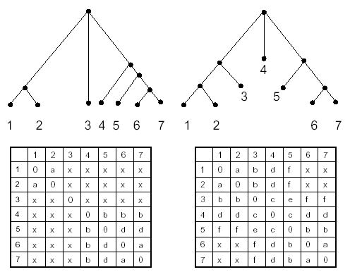
Example illustrating that matrix entropy can be a misleading measure of tree complexity. Contrary to Ramani and Marcotte’s hypothesis, the first tree with a smaller matrix entropy (9.62) is more complex than the second tree with a larger matrix entropy (17.41). Our measure (topological entropy) of 4 and 8 for the respective trees gives an accurate estimation of tree complexity in this case (the smaller the topological entropy, the more complex the tree is).

3 MATERIALS AND METHODS

3.1 Interaction datasets

Our dataset of known protein interaction partners was obtained from Ramani and Marcotte (2003). T-Coffee (Notredame et al., 2000) was used to align sequences from SwissProt (Bairoch and Apweiler, 1997). Similarity matrices and phylogenetic trees from the multiple sequence alignment were computed using CLUSTALW v1.83 (Thompson et al., 1994). Entry X_ij in the similarity matrix denotes the evolutionary distance between proteins i and j in a family after corrections for multiple mutations per amino acid residue (Kimura, 1983). As in Ramani and Marcotte (2003), Chemokine interactions were defined as described in Oppenheim and Feldmann (2001) and other interactions according to the KEGG database v22.0 (Kanehisa, 1996).

3.2 Searching the automorphism space

In practice, the phylogenetic trees of two interacting protein families are often not isomorphic despite looking so to the eye (Fig. 5). In addition, they often contain edges (internal) that are not well supported with high bootstrap values. Such edges are not reliable and are sometimes misleading when it comes to depicting the correct evolutionary relationship between proteins. Thus, MORPH does not place high confidence on these edges, and it solves this problem by contracting/shrinking edges with bootstrap values below a certain cutoff. There is a tradeoff involved in choosing the cutoff value. A higher cutoff could lead to over-shrinking of the tree, resulting in a loss of valuable topological information. A smaller cutoff will preserve the topological information, but since the phylogenetic tree topology is not completely trustworthy (Fig. 4), one might actually end up comparing isomorphic, but misleading, trees. After extensive experimentation, we set the cutoff to 80%. Figure 4 illustrates an example where a cutoff value of 80% will shrink edges with bootstrap values {40, 41} and {48, 73, 76} from the left and right subtrees, respectively. During this shrinking process, we ensure that equal numbers of edges are shrunk on both trees. To achieve this, we shrink the edge with bootstrap value 90 from the left subtree. The resulting trees in this case are not isomorphic. If the resulting trees are not isomorphic, we further contract edges, in increasing order of the bootstrap values, on both trees until the trees are isomorphic.

Fig. 5.

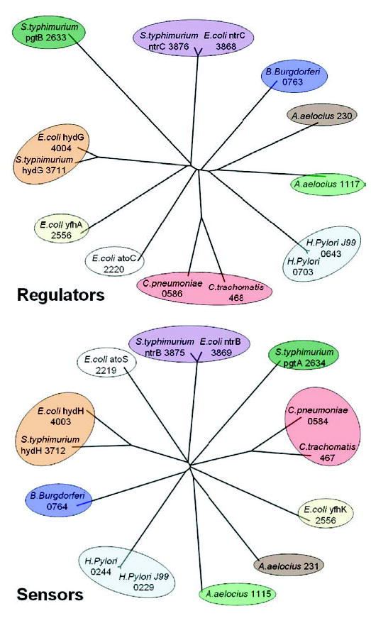
Phylogenetic trees of Ntr-family two-component sensor histidine kinases and their corresponding regulators.

Fig. 4.

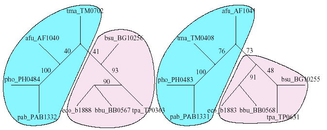
Evolutionary trees (not drawn to scale) of cheA–bacteria and cheB–bacteria obtained from multiple sequence alignment using CLUSTALW v1.83. The numbers along the internal edges represent the bootstrap values of the edges. The tree topologies are clearly different, defying the hypothesis that the evolutionary trees of families (that are known to interact) have similar topologies. Even though the corresponding left subtrees are topologically identical, the positioning of ‘tma_TMxxxx’ and ‘afu_Afxxxx’ proteins is not the same.

Once the trees are isomorphic, we search the tree automorphism space using a Monte Carlo algorithm. Our algorithm keeps one of the two trees (and the corresponding similarity matrix) frozen while performing elementary moves on the other tree (and its matrix). Each point of the search space corresponds to a topology-preserving mapping of the variable tree onto the frozen tree. Thus, each move has to go from one topology-preserving embedding to another topology-preserving embedding. In other words, each move has to go from one automorphism of the variable tree to another.

To compute all possible moves we need to identify all possible symmetries of the variable tree, i.e. all isomorphic subtrees. Given a rooted tree, all isomorphic subtrees can be quickly computed (in time linearly proportional to the number of vertices) (Aho et al., 1974). Once all isomorphic subtrees are identified, we define the move-set. Every move in the move-set constitutes two isomorphic subtrees adjacent to a common node. Consequently, every Monte Carlo step in our algorithm picks a move from the move-set, uniformly at random, and swaps the two subtrees using the Metropolis criterion, resulting in a topology-preserving embedding of the variable tree (Fig. 6).

Fig. 6.

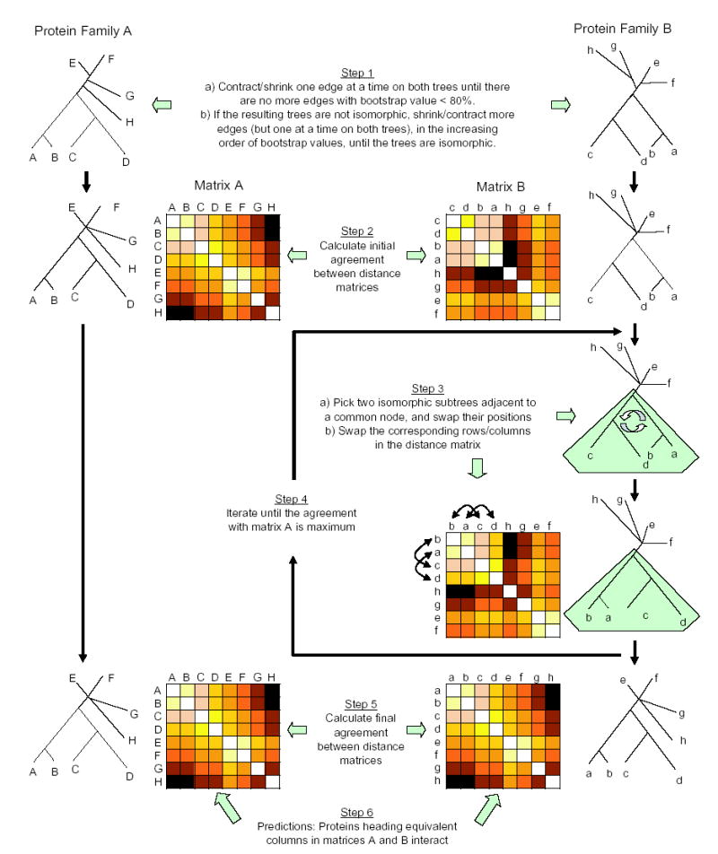
Schematic representation of the MORPH algorithm.

3.3 Methodology

The extent of agreement/superposition of similarity matrices R and S was evaluated using the information theoretic-based measure correlation coefficient (r), given by

$$r=\frac{{\sum }_{i=1}^n(R_i-\overline{R})(S_i-\overline{S})}{\sqrt{{{\sum }_{i=1}^n(R_i-\overline{R})}^2}\sqrt{{{\sum }_{i=1}^n(S_i-\overline{S})}^2}},$$

where n is the number of entries in the matrices, i.e. n = (N² − N)/2, with N being the number of protein sequences in the multiple sequence alignments, and $\overline{R}$ and $\overline{S}$ are the means of all R_i and S_i values, respectively. The value of r ranges from −1 to +1, with higher r indicating greater agreement between the two matrices.

As depicted in Figure 6, MORPH performs necessary contraction of internal edges on the phylogenetic trees of the interacting families until they are isomorphic. It then freezes the first phylogenetic tree and its corresponding matrix while it performs elementary moves on the second tree and its corresponding matrix. The Monte Carlo algorithm with simulated annealing is used to navigate through the search space and maximize the agreement between the two trees/matrices. Each step (move) in the search process constitutes picking two isomorphic subtrees (connected to a common parent) of the variable tree, uniformly at random, and swapping their respective positions. The corresponding columns in the variable matrix are swapped as well. If the performed move results in a better agreement (increased r), the swap is kept. Otherwise, the move is kept with probability p = exp(δ/T), where δ is the decrease in r as a result of the move, and T is the temperature control variable governing the simulated annealing process. T is initially set to a value such that p = 0.8 to begin with, and after each iteration T is decreased by 5%. Once the probability of accepting a decrease falls below 10%, the algorithm initiates the sampling process. In the sampling process, 100 snapshots of the variable similarity matrix are recorded at M step intervals, where M is the number of unique moves that can be performed on the tree. Proteins heading equivalent columns in the frozen matrix and the snapshot of the variable matrix are predicted to interact. From these 100 snapshots, the frequency of a given protein pair interaction is calculated. Then, every protein represented in the frozen matrix is predicted to interact with the most frequently paired protein in the variable matrix. For consistency and reproducibility of the predictions, the algorithm was run 10 times, producing a total of 1,000 snapshots.

4 RESULTS AND DISCUSSION

4.1 Results

The phylogenetic trees of two interacting protein families, the Ntr-type two-component regulators and their corresponding sensors, are shown in Figure 5. At first sight, the trees look topologically similar. The ntrC and hydG proteins from Escherichia coli in the regulator tree are next to the ntrC and hydG proteins from Salmonella typhimurium, respectively. Their corresponding interaction partners in the sensor tree, the ntrB and hydH proteins from E.coli and S.typhimurium, have identical topological relationship. On a closer examination, one can see that the trees are, in fact, not identical. For example, the topological relationships among Borrelia burgdorferi, Aqcuifex aeolicus and Helicobacter pylori proteins are not the same on both trees.

For the Ntr-type two-component sensor and regulator families, there are a total of 14 interaction pairs according to the KEGG database, spanning genes from 8 organisms. MORPH was used to align the two trees/matrices, and the cumulative results of 10 runs are presented in Figure 7. Each entry in the prediction matrix on the left represents the number of times a given protein pair was predicted to interact out of 1000 snapshots from 10 runs, and each entry in the matrix on the right represents the number of times (out of 10 runs) the matrix alignment with maximal agreement predicted interaction of the given pair of proteins. Proteins are arranged such that the main diagonal corresponds to correct binding partners. The matrix on the right in Figure 7 predicts 8/14 binding partners correctly, and the one on the left predicts 10/14 pairs correctly. The incorrect predictions can be justified if one takes a closer look at the branch lengths of the incorrect pairings (Fig. 4). For example, the two A.aeolicus proteins from the sensor family are correctly predicted to interact with the two A.aeolicus proteins from the regulator family, but in the wrong order. Topologically, the predictions are correct since the longer branch (A.aeolicus 230) from the regulator family is predicted to interact with its longer counterpart (A.aeolicus 1115) from the sensor family, and the shorter branch (A.aeolicus 1117) from the regulator family with its shorter counterpart (A.aeolicus 231) from the sensor family.

Fig. 7.

Predicted interactions between Ntr-type two-component regulators and sensors. The main diagonal of the matrix indicates the correct interacting pairs based on the KEGG database. Each entry in the left matrices represents the number of snapshots (out of 1000) in which the given pair of proteins was predicted to interact. Each entry in the right matrices represents the number of times (out of 10 runs) the matrix alignment with maximal agreement predicted interaction of the given pair of proteins. Boxes in bold represent predicted interaction partners, and regular boxes represent the interaction partners when interactions between orthologs are allowed.

As defined by Ramani and Marcotte (2003), we used two measures to assess the accuracy of predicted interactions: stringent and effective accuracy. Stringent accuracy is defined as the accuracy of exact matches of known binding partners, whereas effective accuracy accepts matching orthologous proteins (i.e. it accepts matching the ntrC protein from E.coli to the ntrB protein from S.typhimurium rather than to the ntrB protein from E.coli). The stringent accuracy for the Ntr-type two-component sensor and regulator families was 71.4% and the effective accuracy was 85.7%. Table 1 summarizes the prediction results for all 34 instances we tested using MORPH. For comparison purposes, the table also contains prediction results from MATRIX (Ramani and Marcotte, 2003). Unlike MORPH, MATRIX uses root mean square difference (r.m.s.d.) to calculate the agreement between the similarity matrices, with the smaller r.m.s.d. indicating better agreement. MORPH’s results remained unchanged when run with r.m.s.d. instead of the correlation coefficient (data not shown).

Table 1.

MORPH’s performance at predicting protein interaction partners between two protein families that are known to interact.

		Effective accuracy (%)		Stringent accuracy (%)		Entropyb			Correlation coefficient
	No.of proteinsa	MATRIXg	MORPH	MATRIXg	MORPH	MATRIXg	MORPH	ICc	Correct pairingd	MORPHe	Shrink Factor (%)f
Interacting protein families
Chemokine/receptor–mouse/human/rat	31	48.4	51.6	12.9	22.6	112.7	44.9	67.8	0.868233	0.870028	57.14
Chemokine/receptor–human	13	NA	NA	23.1	23.1	32.5	26.3	6.2	0.540785	0.812693	90.00
CKR-type chemokine/receptor–mouse/human/rat	18	55.5	55.5	33.3	33.3	52.5	23.9	28.6	0.843352	0.856464	53.30
CCR-type chemokine/receptor–mouse/human	6	100.0	100.0	33.3	33.3	9.5	5.6	3.9	0.884096	0.887253	0.00
Omp-type regulator/sensors–E.coli	14	NA	NA	21.4	21.4	36.3	36.3	0.0	0.387540	0.681353	100.00
Omp-type regulator/sensors–Bacillus subtilis	13	NA	NA	7.7	7.7	32.5	32.5	0.0	0.382881	0.715536	100.00
Omp-type regulator/sensors–5 bacteria	16	43.8	56.3	31.3	56.3	44.3	24.8	19.5	0.889139	0.915159	69.23
Omp-type regulator/sensors–E.coli/B.subtilis	27	NA	NA	18.5	18.5	93.1	93.1	0.0	0.418321	0.655748	100.00
Nar-type regulator/sensors–8 bacteria	22	36.4	9.1	36.4	9.1	69.9	44.9	25.0	0.825362	0.872074	78.95
Ntr-type regulator/sensors–8 bacteria	14	85.7	85.7	57.1	71.4	36.3	18.1	18.2	0.902306	0.907389	63.64
Cit-type regulator/sensors–E.coli/B.subtilis	5	100.0	100.0	100.0	100.0	6.9	3.0	3.9	0.780736	0.780736	0.00
Lyt-type regulator/sensors–E.coli/B.subtilis	4	50.0	100.0	50.0	100.0	4.6	4.6	0.0	0.987242	0.987242	100.00
Two-component sensor/regulators–E.coli	27	NA	NA	7.4	14.8	93.1	93.1	0.0	0.541882	0.706465	100.00
Lyt-, Ple-, and ‘other’-type regulator/sensors–8 bacteria	20	NA	NA	5.0	10.0	61.1	61.1	0.0	0.112060	0.521943	100.00
CheA/CheY–11 bacteria	13	69.2	100.0	69.2	100.0	32.5	21.5	11.0	0.837894	0.838406	80.00
ABC transporter membrane protein 1/2–E.coli	19	NA	NA	26.3	26.3	56.8	36.7	20.1	0.589718	0.683888	87.50
ABC transporter membrane/binding protein–E. coli	17	NA	NA	0.0	17.6	48.3	41.3	7.0	0.625733	0.679630	92.86
ABC transporter membrane protein 1/2–Haemophilus influenzae	14	NA	NA	0.0	28.6	36.3	29.8	6.5	0.430913	0.768785	90.91
ABC transporter membrane/binding protein–H.influenzae	13	NA	NA	7.7h	38.5	35.5	32.5	3.0	0.548655	0.691065	100.00
GyrA/B, ParC/E–α-proteobacteria	20	100.0	100.0	50.0h	50.0	61.1	11.0	50.1	0.992959	0.993684	0.00
GyrA/B, ParC/E–Gram positive bacteria	28	100.0	100.0	17.9h	17.9	97.9	32.0	65.9	0.944774	0.947315	52.00
Single interaction partners from multiple organisms
CheA/CheB–bacteria	8	NA	NA	100.0	100.0	15.3	7.6	7.7	0.962251	0.962285	60.00
Acetyl CoA carboxylase α/β Gram positive bacteria	9	NA	NA	33.3	55.5	18.5	4.6	13.9	0.872684	0.884890	33.33
Acetyl CoA carboxylase α/β proteo bacteria	16	NA	NA	75.0	75.0	44.3	37.3	7.0	0.975810	0.978088	92.31
Succinate CoA synthetase α/β proteo bacteria	22	NA	NA	81.8	81.8	69.9	55.5	14.4	0.897055	0.897446	89.47
Succinate CoA synthetase α/β archaea	13	NA	NA	30.8	38.5	32.5	13.5	19.0	0.917747	0.942711	60.00
GyrA/GyrB–α-proteobacteria	20	NA	NA	70.0h	80.0	61.1	36.5	24.6	0.972145	0.972901	70.59
GyrA/GyrB–Gram positive bacteria	18	NA	NA	50.0	55.5	52.5	11.6	40.9	0.981282	0.981444	40.00
GyrA/GyrB–archaea	10	NA	NA	20.0	20.0	21.8	16.3	5.5	0.808534	0.919128	85.71
Pyruvate dehydrogenase α/β–bacteria	17	NA	NA	52.9	82.4	48.3	27.4	20.9	0.953532	0.961960	78.57
ParC/ParE–bacteria	26	NA	NA	61.5	23.1	88.4	42.5	45.9	0.972655	0.696493	73.91
ParC/ParE–α-proteobacteria	12	NA	NA	66.6	83.3	28.8	7.6	21.2	0.992246	0.992580	11.11
ParC/ParE–Gram positive bacteria	14	NA	NA	57.1	57.1	36.3	8.0	28.3	0.968444	0.972985	27.27
DNA polymerase III E2/E3–bacteria	20	NA	NA	45.0	65.0	61.1	19.3	41.8	0.939153	0.951563	52.94

^aNumber of proteins in a family of interacting proteins (number of columns in the corresponding similarity matrix).

^blog (search space).

^cInformation content.

^dCorrelation coefficient for correct pairing of interaction partners.

^eCorrelation coefficient of the maximal agreement of similarity matrices found by MORPH.

^fPercentage of internal edges in the phylogenetic tree that were shrunk to reach isomorphism.

^gProtein interaction prediction algorithm proposed by Ramani and Marcotte (2003).

^hResults in Ramani and Marcotte (2003) could not be reproduced using their MATRIX web server.

Note, from the results in Table 1, that for families with orthologs (single interaction partners from multiple organisms), the prediction accuracy is appreciably higher than that for families with paralogs. The higher prediction accuracy in this case can be attributed to the background “species tree” information present in the trees. For families with paralogs (top half of Table 1), the prediction accuracy for families with out-paralogs² is higher than that for families with in-paralogs. This is expected, since very high sequence similarity between in-paralogs makes them indistinguishable. Our assessment penalizes for incorrect predictions in this case and this, one can argue, is not necessarily fair. In other words, for families with in-paralogs, one can hope to predict only interacting pairs of clades (A.aelocius proteins in Fig. 4). If one takes this into account while assessing the quality of MORPH’s predictions, the prediction accuracy numbers will be better than in Table 1.

4.2 Discussion

The main idea of co-evolution-based methods is to exploit the tendency for interacting proteins to have similar phylogenetic trees. Rather than finding a maximal agreement between the two phylogenetic trees of interacting proteins, previous methods focused on the maximal agreement of the two corresponding similarity matrices (Goh et al., 2000; Pazos and Valencia, 2001; Gertz et al., 2003; Ramani and Marcotte, 2003), never using the topological information contained in the trees explicitly. Their prediction results were based on how well the matrices agree: the better the agreement, the more likely the predictions are true/reliable. In contrast, our results indicate that better agreement does not necessarily have to translate into better prediction accuracy. For all but one instance, our algorithm found better matrix agreement scores compared with that of correct pairings (note the correlation coefficient values in Table 1). Based on this, we make the following observation: correct pairing of interacting proteins between two phylogenetic trees will result in a high agreement score between the corresponding similarity matrices, but a maximal agreement between the similarity matrices does not necessarily mean correct pairing of interacting proteins between the corresponding phylogenetic trees. Theoretically, maximal agreement of similarity matrices should translate into correct pairing of interacting proteins. However, this cannot be verified in practice as similarity matrices obtained from multiple sequence alignments are an imperfect estimation of evolutionary distances, let alone the approximation of sequence alignments. Therefore, our Monte Carlo algorithm is not only directed toward finding the optimal alignment but also toward sampling the suboptimal solutions so that such cases can be detected. Consequently, our algorithm reports predictions based on how frequently the suboptimal solutions are sampled as opposed to how well the matrices agree. If one were to consider a prediction with ≥50% accuracy to be a successful prediction, we observe that a prediction with agreement score (correlation coefficient) better than 0.86 is highly reliable (Fig. 8).

Fig. 8.

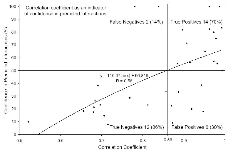
From the correlation coefficient score of the maximal agreement of a given set of similarity matrices, one can say how good/reliable the predictions are. If one were to consider a prediction with ≥50 + % prediction accuracy to be a successful prediction, then a prediction with score 0.86 or more is highly likely to be reliable.

Even though we used T-Coffee to perform the multiple sequence alignments, our algorithm is independent of sequence alignment algorithms as alignments using CLUSTALW and MUSCLE produced comparable results (data not shown). However, there were a few extreme cases. For cheA/cheB–bacteria (shown in Fig. 4), sequence alignment using T-Coffee resulted in an accurate prediction of all eight interaction pairs, whereas sequence alignment using CLUSTALW v1.83 resulted in the correct prediction of only one interacting pair. For Nar-type regulators/sensors, T-Coffee alignment predicted 2 out of 22 interactions correctly, whereas CLUSTALW v1.83 got 8 out of 22 (36.4%) predictions correct. We observed in a few instances that optimal and suboptimal solutions may give superpositions that are almost equally good. In an extreme case (Cit-type regulator/sensors–E.coli/B.subtilis), the difference was so small that whether the global optimum corresponded to the correct pairing of interaction partners depended on the version of the alignment algorithm used. Although CLUSTALW v1.71 accurately predicted all five interaction pairs, CLUSTALW v1.83 was able to predict only three out of five pairs correctly.

There was one instance (ParC/ParE–bacteria) where our greedy shrinking procedure resulted in two isomorphic trees with misleading move-sets. This restricted our algorithm from making the “right” moves, resulting in a lower correlation coefficient score. High shrink factors in Table 1 are often a consequence of MORPH’s greedy shrinking procedure and/or the topologies of the two trees being significantly different. Our current research is directed toward a more systematic shrinking procedure, which we believe will definitely yield better results and, most importantly, faster computing times.

An interesting aspect of our search space and the proposed move-set is that it avoids the high energy barriers apparent in previous approaches. For example, assume that the pair of ‘trees’ in Figure 2(b) has not only identical topology but also an identical set of distances. Because of the tree symmetry, the embedding on Figure 2(b) has a relatively high score but is not optimal. Getting out of this local optimum using the single-column-swapping method used by previous algorithms requires a highly unlikely move—swapping one of the leaves a, b, c with one of the leaves c, d, e (the score after the swap will be significantly worse)—whereas our algorithm can swap whole subtrees in one move. Swapping the subtrees with leaves a, b, c and c, d, e does not encounter any energy barrier, and since it results in a better score, it will be performed with high probability. We confirmed these expectations experimentally by running the corresponding algorithms on such a matrix where the lengths of the three “long” edges were one, and the lengths of the edges within the three 3-edge subtrees were all set to 0.1, 0.15 and 0.2, respectively.

4.3 Computing time

Ramani and Marcotte (2003) note that their column-swapping technique does not guarantee the correct solution for large matrices (>15 proteins) because of the enormous search space they consider in their algorithm. As a compromise, they propose running their algorithm 100 times, and predict that the most frequent protein pairings interact. This results in a running time of ~ 500 min, 5 min for each run, to make predictions on protein families of size 15. For the 34 instances we considered, the average search space reduction by our algorithm, when compared with that of Ramani and Marcotte (2003), is ~363 000-fold. Reduction in search space significantly reduces our algorithm’s computing time, which consequently facilitates solving much larger instances.

References

- Aho AV, Hopcroft JE, Ullman JE. Addison-Wesley; Boston, MA, USA: 1974. The Design and Analysis of Computer Algorithms. [Google Scholar]
- Bairoch A, Apweiler R. The SWISS-PROT protein sequence data bank and its supplement TrEMBL. Nucleic Acids Res. 1997;23:31–36. doi: 10.1093/nar/25.1.31. [DOI] [PMC free article] [PubMed] [Google Scholar]
- Dandekar T, Snel B, Huynen M, Bork P. Conservation of gene order: a fingerprint of proteins that physically interact. Trends Biochem Sci. 1998;23:324–328. doi: 10.1016/s0968-0004(98)01274-2. [DOI] [PubMed] [Google Scholar]
- Gertz J, Elfond G, Shustrova A, Weisinger M, Pellegrini M, Cokus S, Rothschild B. Inferring protein interactions from phylogenetic distance matrices. Bioinformatics. 2003;19:2039–2045. doi: 10.1093/bioinformatics/btg278. [DOI] [PubMed] [Google Scholar]
- Goh CS, Bogan AA, Joachimiak M, Walther D, Cohen FE. Co-evolution of proteins with their interaction partners. J Mol Biol. 2000;299:283–293. doi: 10.1006/jmbi.2000.3732. [DOI] [PubMed] [Google Scholar]
- Goh CS, Cohen FE. Co-evolutionary analysis reveals insights into protein–protein interactions. J Mol Biol. 2002;324:177–192. doi: 10.1016/s0022-2836(02)01038-0. [DOI] [PubMed] [Google Scholar]
- Huynen MA, Bork P. Measuring genome evolution. Proc Natl Acad Sci. 1998;95:5849–5856. doi: 10.1073/pnas.95.11.5849. [DOI] [PMC free article] [PubMed] [Google Scholar]
- Kanehisa M. Toward pathway engineering: a new database of genetic and molecular pathways. Sci Technol Jpn. 1996;59:34–38. [Google Scholar]
- Kimura M. Cambridge University Press; 1983. The Neutral Theory of Molecular Evolution. [Google Scholar]
- Marcotte EM, Pellegrini M, Ng HL, Rice DW, Yeates TO, Eisenberg D. Detecting protein function and protein–protein interactions from genome sequences. Science. 1999;285:751–753. doi: 10.1126/science.285.5428.751. [DOI] [PubMed] [Google Scholar]
- Metropolis N, Rosenbluth AW, Teller A, Teller EJ. Simulated annealing. J Chem Phys. 1953;21:1087–1092. [Google Scholar]
- Notredame C, Higgins D, Heringa J. T-Coffee: a novel method for multiple sequence alignments. J Mol Biol. 2000;302:205–217. doi: 10.1006/jmbi.2000.4042. [DOI] [PubMed] [Google Scholar]
- Oppenheim JJ, Feldmann M. Chemokine Reference. Academic Press; San Diego, CA, USA: 2001. Cytokine reference, a compendium of cytokines and other mediators of host defense. [Google Scholar]
- Overbeek R, Fonstein M, D’Souza M, Pusch GD, Maltsev N. Use of contiguity on the chromosome to predict functional coupling. In Silico Biol. 1998;1:93–108. [PubMed] [Google Scholar]
- Pazos F, Helmer-Citterich M, Ausiello G, Valencia A. Correlated mutations contain information about protein–protein interaction. J Mol Biol. 1997;271:511–523. doi: 10.1006/jmbi.1997.1198. [DOI] [PubMed] [Google Scholar]
- Pazos F, Valencia A. Similarity of phylogenetic trees as indicator of protein–protein interaction. Protein Eng. 2001;14:609–614. doi: 10.1093/protein/14.9.609. [DOI] [PubMed] [Google Scholar]
- Pazos F, Valencia A. In silico two-hybrid system for the selection of physically interacting protein pairs. Proteins. 2002;47:219–227. doi: 10.1002/prot.10074. [DOI] [PubMed] [Google Scholar]
- Pellegrini M, Marcotte EM, Thompson MJ, Eisenberg D, Yeates TO. Assigning protein functions by comparative genome analysis: protein phylogenetic profiles. Proc Natl Acad Sci. 1999;96:4285–4288. doi: 10.1073/pnas.96.8.4285. [DOI] [PMC free article] [PubMed] [Google Scholar]
- Ramani AK, Marcotte EM. Exploiting the co-evolution of interacting proteins to discover interaction specificity. J Mol Biol. 2003;327:273–284. doi: 10.1016/s0022-2836(03)00114-1. [DOI] [PubMed] [Google Scholar]
- Sonnhammer EL, Koonin EV. Orthology, paralogy and proposed clasification for paralog types. Trends Genet. 2002;18:619–620. doi: 10.1016/s0168-9525(02)02793-2. [DOI] [PubMed] [Google Scholar]
- Thompson J, Higgins D, Gibson T. CLUSTALW: improving the sensitivity of progressive multiple sequence alignment through sequence weighting, position-specific gap penalties and weight matrix choice. Nucleic Acids Res. 1994;22:4673–4680. doi: 10.1093/nar/22.22.4673. [DOI] [PMC free article] [PubMed] [Google Scholar]
- Valencia A, Pazos F. Prediction of protein–protein interactions from evolutionary information. Methods Biochem Anal. 2003;44:411–426. [PubMed] [Google Scholar]