

Abstract
Reconstructing low-dose X-ray CT (computed tomography) images is a noise problem. This work investigated a penalized weighted least-squares (PWLS) approach to address this problem in two dimensions, where the WLS considers first- and second-order noise moments and the penalty models signal spatial correlations. Three different implementations were studied for the PWLS minimization. One utilizes a MRF (Markov random field) Gibbs functional to consider spatial correlations among nearby detector bins and projection views in sinogram space and minimizes the PWLS cost function by iterative Gauss-Seidel algorithm. Another employs Karhunen-Loève (KL) transform to de-correlate data signals among nearby views and minimizes the PWLS adaptively to each KL component by analytical calculation, where the spatial correlation among nearby bins is modeled by the same Gibbs functional. The third one models the spatial correlations among image pixels in image domain also by a MRF Gibbs functional and minimizes the PWLS by iterative successive over-relaxation algorithm. In these three implementations, a quadratic functional regularization was chosen for the MRF model. Phantom experiments showed a comparable performance of these three PWLS-based methods in terms of suppressing noise-induced streak artifacts and preserving resolution in the reconstructed images. Computer simulations concurred with the phantom experiments in terms of noise-resolution tradeoff and detectability in low contrast environment. The KL-PWLS implementation may have the advantage in terms of computation for high-resolution dynamic low-dose CT imaging.
I. Introduction
Low-dose X-ray computed tomography (CT) imaging is clinically desired and has been under investigation in the last decade [1]. Reconstructing the low-dose CT images is essentially a noise problem. Up to now, many noise-reduction strategies have been proposed to address this problem. One of the major strategies models the data noise property by a cost function in image space and then minimizes the cost function for image reconstruction by iterative numerical algorithms [2, 3]. An alternative strategy models the noise property by a cost function in sinogram space, seeks an optimal solution for the Radon transform, and then inverts the Radon transform for image reconstruction by filtered backprojection (FBP) algorithm [4–7]. These two strategies of modeling the data statistics are mathematically equivalent with different implementations. Another major strategy applies a sophisticated linear or non-linear filter directly on either sinogram image, ramp-filtered sinogram image [8–12], or reconstructed image [13, 14] which considers the image characteristics rather than the data properties.
Based on repeated phantom experiments, low-mA (or low-dose) CT calibrated projection data after logarithm transform were found to follow approximately a Gaussian distribution with a nonlinear dependence between the sample mean and sample variance, i.e., the noise is signal-dependent [15]. The sample mean and variance dependence can be described by an analytical formula [5, 15]. Filtering this signal-dependent noise by spatially-invariant low-pass filters, such as the Hanning, Butterworth, etc, has shown ineffectiveness, as expected [5, 15]. Sophisticated edge-preserving noise filtering by the use of the local statistics can improve the results [10, 13], but was observed incapable to handle the noise-induced streak artifacts, which mimics the edges [16]. Modeling the signal-dependent noise properties with penalized weighted least-squares (PWLS) cost function in either sinogram space [4, 5] or image domain [17] has shown very promising results. Minimizing the PWLS cost function can be performed iteratively in the image domain for direct image reconstruction [17] or either analytically [4] or iteratively in the sinogram space [5], followed by FBP for image reconstruction. This work reformulated and implemented these three different PWLS minimization approaches [4, 5, 17] by a same quadratic functional regularization. Low-mA CT projection data were acquired from physical (or anthropomorphic) phantoms and also were simulated from digital phantoms to compare the performances of these three different PWLS approaches.
II. Materials and Methods
1. Noise Model
Analysis of repeated measurements from the same phantom indicates that the calibrated and log-transformed projection data of low-mA CT protocol follow approximately a Gaussian distribution with an associated relationship between the data sample mean and variance which can be described by the following analytical formula [5, 15]:
| (1) |
where qi is the mean and σ i2 is the variance of the repeated measurements of projections (after system calibration and logarithm transform) at detector channel or bin i, η is a scaling parameter and fi is a parameter adaptive to different detector bins. Further analysis on the repeated measurements reveals that there is no statistical correlation for the data noise among the detector bins at all the projection views, see Appendix A. These observations on the first- and second-order noise moments lead to the well-known weighted least-squares (WLS) cost function
| (2) |
in the sinogram space and
| (3) |
in the image domain to address the noise problem of low-dose CT imaging, where q = Pμ is the vector of ideal projection data { qi } to be estimated and μ is the vector of attenuation coefficients { μ j } to be reconstructed. Operator P represents the system or projection matrix and the elements of pij is the length of the intersection of projection ray i with pixel j. Vector is the system-calibrated and log-transformed projection measurements. Σ is a diagonal matrix with the i-th element of σ i2, i.e., an estimate of the variance of repeatedly measured at detector bin i which is determined from equation (1). The elements of the diagonal matrix play the weighting role in the WLS cost function. Symbol ′ denotes the transpose operator.
2. Penalized Re-Weighted Least-Squares Image Reconstruction in Image Domain
Minimizing the WLS cost function of equation (2) or (3) usually leads to unacceptable results, similar to the maximum likelihood (ML) approach [18]. A penalty is desired for a penalized ML (pML) or MAP (maximum a posteriori probability) solution [6]. PWLS approach for iterative reconstruction of X-ray CT images has been studied by Herman [19] and Sauer and Bouman [17]. Fessler [20] extended the iterative PWLS image reconstruction to PET (positron emission tomography). Sukovic and Clinthorne [21] applied the iterative PWLS approach in image domain to dual-energy X-ray CT reconstruction. Mathematically, the PWLS cost function can be written, in the image domain, as [17, 20]:
| (4) |
The first term in equation (4) is the WLS measure of equation (3). The second term is a penalty, where β is a smoothing parameter which controls the degree of agreement between the estimated and the measured data. In this work, a quadratic penalty is adapted [20],
| (5) |
where index j runs over all image elements in the image domain, Nj represents the set of eight neighbors of the j-th image pixel in two dimensions. In the two-dimensional (2D) case, the parameter wjm is equal to 1 for the vertical and horizontal first-order neighbors and 1/√2 for the diagonal (second-order) neighbors. The task for image reconstruction is to estimate the attenuation coefficient distribution map μ from the calibrated projections :
| (6) |
In this work, we adapt the iterative successive over-relaxation (SOR) algorithm [20] to calculate the solution of equation (6). In our iterative implementation, the variance σi2 or weight is updated in each iteration according to equation (1) for a more accurate estimation of the projection variance, while in previous work [17, 20] the weight is pre-computed and then fixed for all iterations. To emphasize this difference between our implementation and previously developed iterative PWLS algorithms, we refer our implementation as penalized re-weighted least-squares (PRWLS) algorithm. The intention to update the weight during iteration is to fully utilize the noise model of equation (1) which is established by repeated experimental measurements. The initial variance of each projection datum is estimated by equation (1) from the corresponding noisy projection datum and is updated in each iteration by the newly estimated projection datum. The iterative process is terminated if certain convergence criteria are satisfied for a relatively stable solution [17, 20]. Implementation of the iterative PRWLS+SOR algorithm, similar to that in [20], for our low-dose CT image reconstruction can be summarized as follows:
| (7) |
where 0 ≤ ω ≤1. If ω is set to 1, the above procedure is equivalent to the Gauss-Seidel (GS) update algorithm as described in [17].
3. Penalized Re-Weighted Least-Squares Noise Reduction of Sinogram Data
Another statistical image reconstruction strategy is to find an optimal estimation of the line integral or the Radon transform from the noisy sinogram, and then reconstruct the CT image by FBP method, which is theoretically derived for the inversion of the Radon transform. This statistical approach in sinogram space is more computationally efficient than the statistical reconstruction through the image domain. The PWLS cost function in the sinogram space can be described by:
| (8) |
where q is the vector of ideal projection data (as defined before), the first term is the WLS measure of equation (2), and R(q) is the penalty term similar to equation (5), i.e.,
| (9) |
where Ni indicates the set of four nearest (or first-order) neighbors of the i-th pixel in the sonogram ((or a 2D projection image from a 2D object). The parameter wim is equal to 1 for the two horizontal neighbors (along the bin direction) and 0.25 for the two vertical neighbors (along the angular direction) [5]. By this design, the sinogram is smoothed less in the angular direction than in the radial direction. The task for sinogram noise reduction is to estimate q from :
| (10) |
There are many numerical algorithms which can be employed to calculate the solution of equation (10). In this work, we adapt the iterative GS update algorithm as used in [5, 17]. Our iterative formula for the solution of equation (10) is given by:
| (11) |
where index n represents the iterative number, Ni1 denotes the upper and left neighbors of qi, Ni2 denotes the right and lower neighbors of qi, and Ni denotes these four neighbors of qi. In our implementation, the variance σi2 or weight is updated in each iteration according to equation (1) in a same manner as that of iterative PRWLS+SOR algorithm above and, therefore, we refer our iterative implementation in sinogram space as GS-PRWLS algorithm.
Implementation of the iterative GS-PRWLS sinogram noise reduction approach for the solution of equation (10) can be summarized as follows:
Initialize an estimate of the noise-free sinogram from the calibrated measurements .
Update the previous estimate in a pixel-by-pixel manner based on equation (11).
Update the variance σi2 according to equation (1).
Repeat step 2 and 3 until it converges to a relatively stable solution measured by certain criteria, which are usually determined empirically [17, 20]. In our experiments, 20 iterations are usually sufficient for a stable estimation, which does not change visually for further iterations.
4. Penalized Weighted Least-Squares Sinogram Noise Reduction in KL Domain
In the PRWLS+SOR approach, the penalty is implemented in the image domain for direct image reconstruction. The GS-PRWLS approach implements the penalty in the sinogram space for ideal sinogram estimation, followed by FBP for image reconstruction. The penalty plays a very important role and assumes implicitly some kind of data signal correlations in either image domain or sinogram space. By analyzing the repeated phantom measurements, we observed a strong data signal correlation among the nearby views, see Appendix B. This correlation can be effectively utilized by the Karhunen-Loève (KL) transform for two purposes. One is to decomposite the correlated signals for adaptive noise treatment and the other is to reduce the above 2D sinogram noise-filtering operation into a series of 1D procedures, each on a KL principal component, respectively.
In this study, the KL transform is first applied to account for the correlative information among the nearby views of tomographic projections as reported in [4]. For each (or v-th) view of the projection data, its nearby views (i.e., n views before the v-th view and n views after the v-th view, n = 1, 2, 3, …) are selected to perform the KL transform. For the nearby 2n+1 views, the element kl of the covariance matrix Kt of the projection data can be calculated by [4, 22]:
| (12) |
where yi,k is the datum of sinogram at detector bin i and view angle k, yi,l is the datum of at detector bin i and view angle l,
| (13) |
and B is the number of bins for each view and index k or l runs over the nearby views.
From the covariance matrix Kt, the KL transform matrix A is calculated based on
| (14) |
In equation (14), D = diag {dl }l =12n+1, where d l is the l-th eigenvalue of K t. The dimension of Kt is usually very small so that the eigenvector in equation (14) can be very efficiently computed. In this work, n is chosen to be 1 so that the dimension of matrix Kt is 3×3, (i.e., k, l = 1, 2, 3). The KL transform is then defined as:
| (15) |
where denotes the KL transformed . After the KL transform, the covariance of will be:
| (16) |
where all of the symbols have been defined previously. Equation (16) implies that the covariance matrix of the KL transformed data signal is diagonal, i.e., the covariance of the signal between different views after the KL transform will be zero. Therefore, the data signals of different KL components are no longer correlated so that PWLS objective function can be constructed for each KL principal component separately. For each principal component in the KL domain, the PWLS cost function can be expressed, from the WLS of equation (2), as [4, 22]:
| (17) |
where and are the l-th KL components of and q respectively, is the penalty term which will be defined later and is the diagonal variance matrix of . The inverse variance matrix can be estimated by [4, 22]:
| (18) |
where Qi = diag{σ i,k2 }k=12n+1 is the variance matrix of the projection at bin i, σi,k2 is the variance of yi,k, and ϕl is the l-th KL basis vector. For a given pixel in the sinogram, a 3×3 window has been used to estimate the sample mean, then the estimated sample mean can be employed by equation (1) to calculate the sample variance σi,k2 for the weight with excellent results [4]. Equation (17) reveals that the regularization parameter shall be chosen as ( β/dl ), so that the PWLS minimization becomes adaptively to each KL component. This choice is favorable because the regularization parameter varies adaptively according to the SNR (signal-to-noise ratio) of that component. A smaller KL eigenvalue is usually associated with a component having a lower SNR and, therefore, a larger regularization value shall be used to penalize this noisier data component [4, 22]. By the KL transform along the angular direction, the above 2D sinogram noise reduction now becomes a 1D process on each principal component, where the 1D process is performed along the bin direction [4]. For the 1D process along the bin direction, the quadratic penalty in equation (17) can be defined as:
| (19) |
where Ni indicates the two nearest neighbors of the i-th pixel in the KL domain along the 1D bin direction (i.e., m = i ±1) and the parameter wim is equal to 1 for the two neighbors. This penalty considers the data signal correlation among nearby bins and plays the same role as the penalty terms in the above PRWLS+SOR and GS-PRWLS approaches.
Taking the derivative of equation (17) with respect to in the KL domain, minimizing equation (17) becomes solving from the following tri-diagonal system of equations of
| (20) |
where is a tri-diagonal matrix of
| (21) |
with dimension of B×B, where B was defined before as the number of detector bins of each view.
For the tri-diagonal equation sets of equation (20), the solution of can be computed analytically and efficiently through the procedures of LU decomposition [23]. After the PWLS noise treatment for each component in the KL domain, the processed data are inverse KL transformed, followed by FBP reconstruction for the low-dose CT images.
Implementation of our analytical KL-PWLS sinogram noise-reduction approach for low-dose CT application can be summarized as follows:
For a chosen v-th view from the calibrated projection data, the (v−1)-th and the (v+1)-th views of the projections are selected for the KL transform.
Compute the spatial covariance matrix Kt from the selected neighboring views of the projections according to equation (12).
Calculate the KL transform matrix A according to equation (14). (4) Apply the KL transform on the selected neighboring views.
Perform PWLS minimization on each KL component via equation (20).
Apply inverse KL transform on the processed KL components for the estimate of the ideal sinogram at the chosen v-th view.
Let v run from 1 to V for the restoration of whole sinogram, where V is the number of views of the sinogram.
The estimated ideal sinogram by either iterative GS-PRWLS or analytical KL-PWLS minimization is then reconstructed by FBP algorithm, which is well established for the inversion of the Radon transform by both speed and consistence.
III. Results
1. Experimental Results
To compare the above three different PWLS-based strategies for noise reduction for low-dose CT imaging, projection datasets from two different phantoms were acquired by a GE Hi-Speed multi-slice CT scanner with 10 mA and 20 mA respectively. The number of bins per view is 888 with 984 views evenly spanned on a circular orbit of 360°. The detector arrays are on an arc concentric to the X-ray source with a distance of 949.075 mm. The distance from the rotation center to the X-ray source is 541 mm. The detector cell spacing is 1.0239 mm. The reconstructed image is of 512×512 array size.
For comparison purpose, reconstructed images by a conventional FBP method (i.e., using a spatially-invariant low-pass Hanning filter with cutoff at 80% Nyquist frequency -- selected by visual inspection for a good result) are shown in Fig. 1(a) (from the Shoulder phantom) and Fig. 4(a) (from the GE QA phantom). From the 10 mA Shoulder phantom study of Fig. 1, severe noise-induced streak artifacts has been observed in the conventional FBP reconstructed image, no matter what a cutoff frequency was used. Images reconstructed by the PRWLS+SOR approach after 40 iterations are shown in Fig. 1(b) and Fig. 4(b). (The choice of 40 iterations has also been shown to produce a relatively stable solution, which did not change visually for further iterations [17, 20]). Standard FBP (with Ramp at the Nyquist frequency cutoff) reconstructed images from the GS-PRWLS smoothed sinograms (after 20 iterations) are shown in Fig. 1(c) and Fig. 4(c). (The choice of 20 iterations has also been shown to produce a relatively stable solution, which did not change visually for further iterations). Standard FBP reconstructed images from the analytical KL-PWLS filtered sinograms are shown in Fig. 1(d) and Fig. 4(d). To further illustrate the effectiveness of these PWLS-based approaches, zoomed images of a ROI (region of interest) are shown in Fig. 2 and Fig. 5 for the Shoulder and QA phantom respectively. For these three PWLS-based methods, we tried various penalty parameters to ensure they have matched resolution as much as possible. Figure 3 illustrates the vertical profiles along an edge in the reconstructed images of the 10 mA Shoulder phantom using the PWLS-based methods, where the profiles match closely to each other.
Fig. 1.
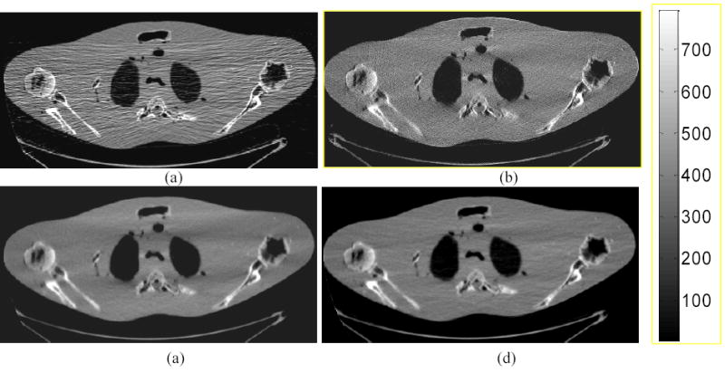
Shoulder phantom study with 10 mA protocol. (a): A conventional FBP reconstructed image using the Hanning filter with cutoff at 80% Nyquist frequency. (b): Iterative PRWLS+SOR reconstructed image with β =1×10⁻⁴. (c): A standard FBP reconstructed image from the iterative GS-PRWLS smoothed sinogram with β =1×10⁻⁸. (d): A standard FBP reconstructed image from the analytical KL-PWLS filtered sinogram with β =200.
Fig. 4.
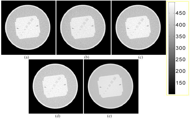
QA phantom study with 20 mA protocol. (a): A conventional FBP reconstructed image using the Hanning filter with cutoff at 80% Nyquist frequency. (b): Iterative PRWLS+SOR reconstructed image with β =1×10⁻⁴. (c): A standard FBP reconstructed image from the iterative GS-PRWLS smoothed sinogram with β =1×10⁻⁸. (d): A standard FBP reconstructed image from the analytical KL-PWLS filtered sinogram with β =200. (e): A standard FBP reconstructed image by the Ramp filter with 100% Nyquist frequency from the average of 19 repeated measurements (it is assumed as the gold standard in this phantom experiment).
Fig. 2.
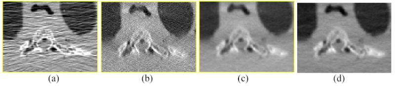
Zoomed images of a ROI from the corresponding images of Fig. 1: (a) Result from Hanning filter; (b) from the PRWLS+SOR strategy; (c) from the GS-PRWLS strategy; and (d) from the KL-PWLS strategy.
Fig. 5.
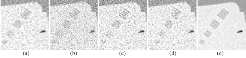
Zoomed images of the sets of strip bars from the corresponding images of Fig. 4: (a) Result from the Hanning filter; (b) from the PRWLS+SOR strategy; (c) from the GS-PRWLS strategy; (d) from the KL-PWLS strategy; and (e) from the average of 19 repeated measurements (as the gold standard).
Fig. 3.
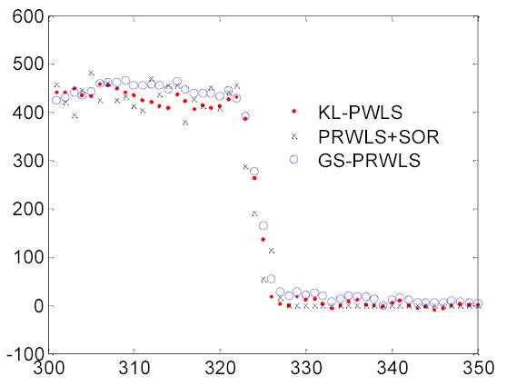
Vertical profiles through the reconstructed images of the three PWLS-based methods.
All these three PWLS minimization reconstructions removed satisfactorily the noise-induced streak artifacts as shown in Figs. 1, 2 and 3. Manipulating the cutoff frequency of the Hanning filter in a conventional FBP reconstruction could not reach a comparable noise-resolution tradeoff as that of the three PWLS approaches. At a higher cutoff frequency, the Hanning filter produced a noisy result, while at a lower cutoff frequency, the edge details were significantly smoothed out. In contrary, excellent noise reduction with satisfactory resolution preservation of the PWLS-based strategies was observed. This excellent performance of PWLS-based algorithm was also seen in Figs. 4, 5 and 6. From Fig. 6, it can be observed that the five largest air strips between pixel 80 and pixel 95 are well preserved by all of the three PWLS-based algorithms while some of the air strips are disappeared by the use of the Hanning filter. Lowering the cutoff frequency of the Haning filter could not recover the missed air strips except for increasing the noise level. Compare to the gold standard of reconstruction from the average of 19 repeated measurements, the Hanning filter could not reach the noise-resolution tradeoff of the PWLS-based approaches by manipulating its cutoff frequency. This observation was also reported in the previous work [4, 5, 14, 24].
Fig. 6.
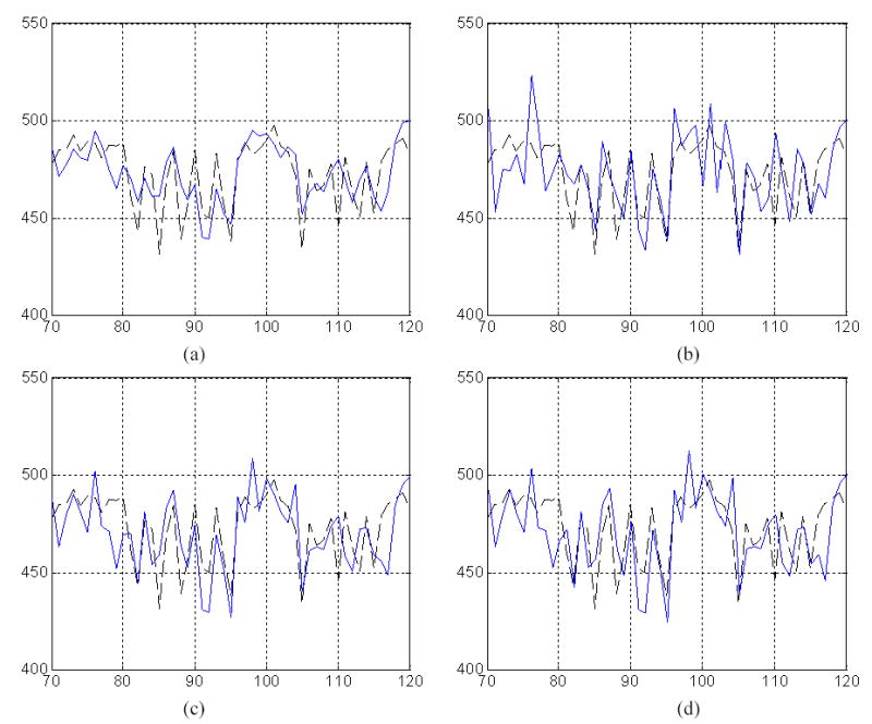
Profiles of two-pixel-width through the sets of the small strips in images of Fig. 4. The “solid-line” in (a) is from the Hanning filter, (b) from the PRWLS+SOR strategy, (c) from the GS-PRWLS strategy and (d) from the KL-PWLS strategy. The “dashed-line” in all of above figures is from the average of 19 repeated measurements (i.e., the gold standard).
2. Resolution-Noise Tradeoffs
The noise-resolution tradeoffs of the presented three PWLS approaches were computed by computer simulation using an ellipse digital phantom of Fig. 7(left) similar to that one used in [6, 9]. The detector array and X-ray source configuration is exactly the same as the GE scanner as described before. The ellipse phantom was sampled by the detector system on a circular orbit. Noise-free sinogram was computed based on the known densities and intersection lengths of the projection rays with the geometric shapes of the objects in the phantom. Noisy sinograms were generated by adding signal-dependent Gaussian noise according to equation (1), simulating the low-mA CT data acquisition protocol. Image reconstruction was performed on a 512×512 array size in the image domain.
Fig. 7.
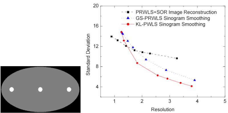
Left is the phantom used for the noise-resolution tradeoff studies. Right shows the noise-resolution tradeoff curves for the presented three PWLS approaches. The resolution is measured by FWHM in pixel units.
The reconstructed image resolution was analyzed by the edge spread function (ESF) along the central vertical profile on the left disk in the reconstructed ellipse-phantom image, which is similar to that used in [6]. The ESF is a measure of the broadening of a step edge. Assume that the broadening kernel is a Gaussian function with standard deviation σb, the ESF can be described by an error function (erf) parameterized by σb. By fitting the vertical profiles through the center of the left disk to an error function, we can obtain the parameter σb. The obtained parameter σb reflects the full-width at half-maximum (FWHM) of the broadening Gaussian function and, therefore, the reconstructed image resolution.
The reconstructed image noise was characterized by the standard deviation of a uniform region around the left disk in the reconstructed ellipse-phantom image. By varying the penalty parameter β for the three different PWLS-based approaches, we obtained the noise-resolution tradeoff curve for each approach. The noise-resolution tradeoff curves are shown in Fig. 7(right). The noise-resolution tradeoff curves of the GS-PRWLS and KL-PWLS sinogram smoothing approaches have the same trend. The KL-PWLS strategy shows a slightly better performance than the GS-PRWLS approach in all the resolution range. This may be due to the consideration of the signal correlation by the KL transform. The noise-resolution tradeoff curve of the PRWLS+SOR image reconstruction is slightly different from the other two approaches. At higher resolution (<1.5), the PRWLS+SOR image reconstruction is better than the PWLS-based sinogram smoothing approaches. At lower resolution (>1.5), the PWLS-based sinogram restoration is better than the PRWLS+SOR image reconstruction. This difference may be due to their implementation of penalty in different spaces. The penalty in PRWLS+SOR is implemented in image domain among the nearby image pixels. It is a local effect on the reconstructed image. However, the penalty of the PWLS minimization in the sinogram space may have a global effect on the FBP reconstructed image. Further investigation for different penalties in the sinogram space is needed.
3. Receiver Operating Characteristic (ROC) Studies by Channelized Hotelling Observer
One generally accepted method for evaluation of the performance of a medical imaging system or procedure is to evaluate the ability of an observer to detect an abnormality. By the observer study, a variety of pairs of true positive fraction (TPF) and false positive fraction (FPF) are generated as an observer changes the confidence threshold, resulting in a ROC curve [25]. Each ROC curve describes the inherent discrimination capacity of an imaging system or procedure. A common merit for comparing the ROC curves is the area under the curve (AUC) or AZ. The reconstruction scheme, which generates a larger AUC, usually reflects a better detectability on abnormality. In this study, the channelized Hotelling observer (CHO) [26] was employed to generate ROC curves. This could eliminate the intra human observer variation.
Figure 8(left) shows a modified Shep-Logan head phantom (256×256 mm2) used for the ROC study, where a low-contrast small lesion grows from the big ellipse as indicated by the arrow in the picture. The density of the lesion is about 1.5% of the background density and the radius of the lesion is 3 mm. The noise-free sinograms of this modified phantom with the lesion and the original phantom without the lesion were simulated, respectively. A total of 250 noisy sinograms were generated from each noise-free sinogram by adding Gaussian noise according to equation (1). Then these noisy sinograms were reconstructed by the three different PWLS-based reconstruction schemes. The CHO [26] gives a rating value for each image. Here we used four octave-wide rotationally symmetric frequency channels proposed by Myers and Barrett [26]. This channel model was found to give good predictions of a human observer study in myocardial defect detection and in comparing fan- and parallel-beam collimators [27, 28]. In this CHO study, each reconstructed image generated a four-element feature vector, and the CHO was trained separately for each PWLS-based reconstruction approach, using subsets of these feature vectors given their class category (i.e., with or without lesion). Then the CHO was applied to a different, independent ensemble of feature vectors to produce an ensemble of scalar rating values, which were subsequently analyzed using the CLABROC code [25], resulting in four pairs of FPF and TPF for each reconstruction method. These four pairs were then fitted by a ROC curve using the bi-normal model. By varying the penalty parameter β, we generated a series of ROC curves for each reconstruction method. The ROC curves of optimized penalty parameters are plotted in Fig. 8(right). The area under the three curves is 0.924 for the PRWLS+SOR image reconstruction, 0.920 for the GS-PRWLS sinogram restoration approach, and 0.925 for the KL-PWLS sinogram restoration strategy. The one-tailed p-values between each pair of two approaches are all larger than 0.05, which indicates that the difference between these three PWLS-based approaches is statistically not significant.
Fig. 8.
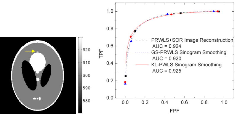
Left picture is the modified Shepp-Logan head phantom used for ROC study. The right picture shows the results of the ROC evaluation and the fitted ROC curves by the binormal model.
4. Comparison Study with Adaptive Trimmed Mean (ATM) Filter
In modern CT systems, the measurements from low-dose scan is usually processed by adaptive filters [9, 12] before logarithm transform. To quantitatively show the advantages of PWLS-based algorithms over local statistics-based adaptive filters, we compared the performance of the GS-PRWLS sinogram smoothing approach with the ATM filter [9] using computer simulations. The GS-PRWLS sinogram smoothing approach was selected as a representative of PWLS-based algorithms because its performance can be regarded as the baseline of the three PWLS-based algorithms studied in this paper.
We first performed the noise-resolution tradeoff studies for the ATM filter on pre-logarithm sinogram and the GS-PRWLS algorithm on log-transformed sonogram using the same noise model in [6, 9]. The phantom used for this study is shown in the left of Fig. 7 and the characterization of noise and resolution is described in Section III-2. To simulate the pre-logarithm noisy sinogram, we first computed the line integrals { qi } using the same geometry and method described in section III-2 and then generated the noisy measurements { Ii } according to the noise model of pre-logarithm sinogram that was described in [6]:
| (22) |
where I0 is the incident X-ray intensity and σe2 is the background electronic noise variance. In this study, I0is set to 2.5 ×10⁵ and σe2 is set to 10 [6]. After the noisy measurements were filtered by the ATM filter [9] with baseline parameter 0.2, the smoothed sinogram was calculated by [6]:
| (23) |
where are the measurements smoothed by the ATM filter and δ is a threshold to enforce that the logarithm transform is applied on positive numbers. In this study δ was chosen as 0.01, which is the same as that in [6]. The smoothed sinogram was reconstructed by FBP for low-dose CT images. By the GS-PRWLS approach, we first calculated the log-transformed noisy sinogram according to equation (23) and then calculated the variance of the log-transformed data according to σi2 = (1 + σe2/Ii)exp(qi)/I0 [9], so that both ATM and GS-PRWLS utilized the same noise model of equation (22). The ideal sinogram was then estimated using the GS-PRWLS algorithm as described in Section II-3. By varying filter length and cutoff parameter in the ATM filter and the penalty parameter β in the GS-PRWLS algorithm, we obtained the noise-resolution tradeoff curves at the left disk of the elliptical phantom (Fig. 7) as shown in Fig. 9. It can be observed that the GS-PRWLS algorithm has a better performance than the ATM filter in all of the resolution range.
Fig. 9.
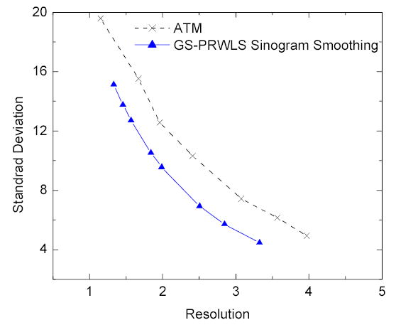
Noise-resolution tradeoff curves of the ATM filter and the GS-PRWLS algorithm.
To evaluate the detectability of the ATM filter and the GS-PRWLS algorithm using the same noise model of equation (22), we performed ROC studies by channelized Hotelling observer. The line integrals of the modified Shepp-Logan head phantom with the lesion (in Fig. 8) and the original phantom without the lesion were computed, respectively. A total 250 pre-logarithm noisy measurements were then simulated according to equation (22) from each line integral. These noisy measurements were processed by the ATM filter, and then the log-transform sinograms were calculated according to equation (23) and reconstructed by FBP method. By the GS-PRWLS approach, we first calculated the log-transformed noisy sinogram according to equation (23) and then estimated the ideal sinogram using the GS-PRWLS algorithm as described in Section II-3. The estimated sinogram was then reconstructed by the same FBP method. The CHO [26] generated a score for each image reconstructed by FBP from the smoothed log-transformed sinograms of ATM and GS-PRWLS. These scores were analyzed using the CLABROC code [25], resulting in four pairs of FPF and TPF for each reconstruction method. The four pairs were then fitted by a ROC curve using the bi-normal model. We tried various filter lengths in the ATM filter and penalty parameters β in the GS-PRWLS, and the best ROC curve for each approach is shown in Fig. 10. The AUC for ATM is 0.871 and for GS-PWLS is 0.917. The one-tailed p-value between these two approaches is less than 0.05 which indicates that the difference between ATM and GS-PRWLS approaches is statistically significant.
Fig. 10.
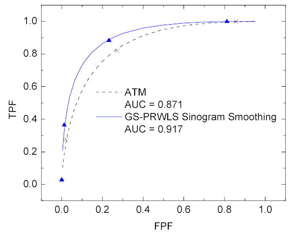
Results of the ROC evaluation and the fitted ROC curves of ATM filter and GS-PRWLS algorithm.
IV. Discussion and Conclusion
Based on the noise properties of calibrated and log-transformed CT sinogram, where the calibration is expected to be well-established for current high-quality CT images, we compared three different PWLS-based noise reduction strategies for low-dose CT application. The PRWLS+SOR strategy is based on the PWLS cost function in image domain and the CT image is reconstructed by minimizing the cost function iteratively with penalty on the neighboring image pixels. The GS-PRWLS and KL-PWLS sinogram noise-reduction approaches aim to estimate the ideal sinogram (or the Radon transform) by minimizing the PWLS cost function with local penalty in sinogram space and reconstruct the CT images by inverting the Radon transform via the standard FBP algorithm (which has been widely used because of its speed and consistence). The GS-PRWLS strategy utilizes the penalty term to consider the difference of neighborhood between angular direction and radial direction (i.e., inside the sinogram) and performs the estimation of the ideal sinogram by the iterative GS update algorithm. The KL-PWLS strategy employs the KL transform to consider the signal correlation among the nearby projections and performs the estimation of the ideal sinogram analytically with penalty on the nearby detector bins, eliminating one freedom/dimension in the penalty (i.e., from 2D to 1D operation). Both phantom experiments and computer simulations demonstrated a similar performance for all these three PWLS-based approaches. The KL-PWLS strategy shows some improvement over the GS-PRWLS, and this may be due to the consideration of signal correlation via the KL transform. The PRWLS+SOR strategy shows some difference on resolution-noise tradeoff from the GS-PRWLS and KL-PWLS strategies, and this may be due to their different implementations of the penalty terms in difference spaces.
All of the three PWLS-based algorithms studied in this paper are based on the noise properties of the log-transformed data of equation (1), which is established by repeated experimental measurements. To obtain the log-transformed sinogram from the raw data of X-ray detector, certain thresholds and/or “tricks” have to be set during the system calibration in order to ensure that the logarithm is applied on positive values,. As an example, if the noise model of equation (22) is considered, then the threshold δ in equation (23) must be considered. This threshold setting could introduce some bias when the X-ray counts are below the electronic noise level.
Based on the noise model of equation (22), a comparison study between the ATM filtration and the GS-PRWLS approach was performed, where the noise-resolution tradeoff and ROC measures indicate a better performance for the PWLS-based algorithms over the adaptive filtration, e.g., the ATM filter. This gain may be due to the use of the noise model by the PWLS-based approaches, rather than the estimation from local statistics in the adaptive filtration.
Alternative to the PWLS strategy and adaptive filtration, the pML approach by modeling the raw data directly (before system calibration and logarithm transform) with maximization in the image domain [3] or in the sinogram space (followed by FBP) [6, 7] have also shown potential for low-dose CT applications. Comparing these pML approaches to the presented PWLS-based strategies would be an interesting research topic and will be investigated. It is worth to investigate the equivalence between the noise model of equation (1) in sinogram space and the compound Poisson noise model of the raw data [29].
The above approaches were presented in 2D case, while clinical applications are usually in three dimensions. Thibault et al. [29] have demonstrated the advantages of iterative image reconstruction for cone-beam artifacts reduction and image quality improvement over conventional techniques in multi-slice helical CT, although computational load of iterative reconstruction is still the challenge for practical development. We have demonstrated the effectiveness of the KL-PWLS sinogram smoothing strategy for noise reduction of single-slice helical CT [31]. To apply the GS-PRWLS or KL-PWLS sinogram smoothing algorithm to multi-slice helical or cone-beam CT, the penalty in sinogram space should be deliberately designed and further investigation on the penalty design is required. August and Kanade [32] has studied the relationship of penalties between image domain and sinogram space, where the penalties in image domain and sinogram space are related by the Riesz potential, and such relationship could be adapted by the GS-PRWLS and KL-PWLS sinogram smoothing algorithms for the applications on 3D multi-slice helical or cone-beam CT [32]. A simple extension of the presented non-iterative KL-PWLS approach to 3D non-cone beam helical CT application would be to apply the KL transform on the nearby views along the helical path.
These three different PWLS-based strategies were coded by C++ language and executed in a PC Pentium IV with 2.4 GHz CPU speed and 2GB RAM memory. The PRWLS+SOR image reconstruction took approximately 10 minutes per iteration. The GS-PRWLS noise reduction in sinogram space took approximately 3 seconds per iteration. The analytical KL-PWLS noise treatment in the sinogram space took approximately 5 seconds. The gain in computing speed by the KL-PWLS strategy can be seen.
Acknowledgments
We would like to thank the anonymous reviewers for their constructive comments and suggestions that greatly improve the quality of the manuscript. We would also appreciate the discussions on this topic with Drs. Jeffrey A. Fessler and Patrick J. La Riviere. This work was supported in part by the National Institutes of Health under Grant #CA082402. Dr. H. Lu was supported by the National Nature Science Foundation of China under Grant 30170278.
Appendix A: Correlation Coefficient of Data Noise among Detector Bins
The statistical correlation coefficient of data noise (i.e., the datum minors its mean) between the i-th and the j-th detector bins is defined by [33]:
| (A.1) |
where cov is the covariance of repeated measurements of projection data between the i-th and the j-th detector bins, σi and σj are the standard deviations for the projection data of the i-th and j-th detector bins respectively. The statistical correlation coefficients matrix of the noise among the detector bins is shown in Fig. A1. Only the diagonal elements have a value of 1, other elements have values close to zero, indicating that there is no correlation among different detector bins.
Fig A1.
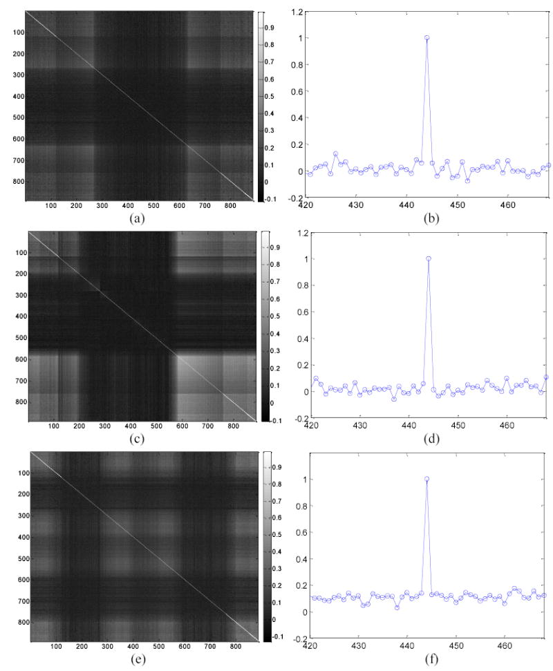
Correlation coefficients matrix of data noise among detector bins from repeated measurements of (a) the QA nearly-symmetric cylinder phantom, (c) the Shoulder asymmetric phantom at 3 o’clock position, and (e) the Shoulder asymmetric phantom at 12 o’clock position. Pictures (b), (d) and (f) show the horizontal profiles through the center of (a), (c) and (e) correspondingly. It can be observed that only the diagonal value is equal to 1 while off-diagonal values are close to zero.
Appendix B: Correlation Coefficient of Data Signal among Projection Views
The correlation coefficient of data signal between the k-th view and the l-th view is defined by [33]:
| (A.2) |
where and were defined by equation (13). Figure A2 shows the correlation coefficients matrix of the signal among the projection views. The values of the diagonal band or diagonal element groups are close to 1, which indicates a strong signal correlation among the neighboring views. Similar results were obtained for the signal among detector bins, which indicates a strong signal correlation among the neighboring detector bins.
Fig A2.
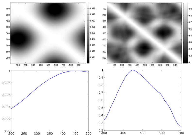
Correlation coefficients matrix of data signal among projection views from the sinogram of the QA nearly-symmetric cylinder phantom (top left) and the asymmetric Shoulder phantom (top right). Bottom shows their horizontal profiles across their centers respectively. The wider range of non-negligible values on bottom left is due to the high symmetric property of the QA phantom, see Fig. 4. The sinogram of the QA phantom is almost uniform along the view direction. Therefore, the correlation coefficients between different views have a wider range of nonnegligible values. When the phantom becomes more asymmetric, such as the Shoulder phantom in Fig. 1, the sinogram becomes more non-uniform along the view direction and, therefore, the correlation coefficients between nearby views have a narrow range of non-negligible values, as shown on the bottom right.
References
- 1.Linton OW, Fred A, Mettler FA. “National conference on dose reduction in CT, with an emphasis on pediatric patients”. American Journal of Roentgenology. 2003;181:321–329. doi: 10.2214/ajr.181.2.1810321. [DOI] [PubMed] [Google Scholar]
- 2.Lange K, Carson R. “EM reconstruction algorithms for emission and transmission tomography”. J Computer Assisted Tomography. 1984;8:306–316. [PubMed] [Google Scholar]
- 3.Elbakri IA, Fessler JA. “Efficient and accurate likelihood for iterative image reconstruction in X-ray computed tomography”. Proc SPIE Med Imaging. 2003;5032:1839–1850. [Google Scholar]
- 4.Lu H, Li X, Hsiao IT, Liang Z. “Analytical noise treatment for low-dose CT projection data by penalized weighted least-squares smoothing in the K-L domain”. Proc SPIE Med Imaging. 2002;4682:146–152. [Google Scholar]
- 5.Li T, Li X, Wang J, Wen J, Lu H, Hsieh J, Liang Z. “Nonlinear sinogram smoothing for low-dose X-ray CT”. IEEE Trans Nucl Science. 2004;51:2505–2513. [Google Scholar]
- 6.La Rivière PJ, Billmire DM. “Reduction of noise-induced streak artifacts in X-ray computed tomography through Spline-based penalized-likelihood sinogram smoothing”. IEEE Trans Med Imaging. 2005;24:105–111. doi: 10.1109/tmi.2004.838324. [DOI] [PubMed] [Google Scholar]
- 7.La Rivière PJ. “Penalized-likelihood sinogram smoothing for low-dose CT”. Med Phys. 2005;32:1676–1683. doi: 10.1118/1.1915015. [DOI] [PubMed] [Google Scholar]
- 8.Sauer K, Liu B. “Non-stationary filtering of transmission tomograms in high photon counting noise”. IEEE Trans Med Imaging. 1991;10:445–452. doi: 10.1109/42.97595. [DOI] [PubMed] [Google Scholar]
- 9.Hsieh J. “Adaptive streak artifact reduction in computed tomography resulting from excessive X-ray photon noise”. Med Phys. 1998;25:2139–2147. doi: 10.1118/1.598410. [DOI] [PubMed] [Google Scholar]
- 10.Demirkaya K. “Reduction of noise and image artifacts in computed tomography by nonlinear filtration of the projection images”. Proc SPIE Med Imaging. 2001;4322:917–923. [Google Scholar]
- 11.Zhong J, Ning R, Conover D. “Image denoising based on multiscale singularity detection for cone beam CT breast imaging”. IEEE Trans Med Imaging. 2004;23:696–703. doi: 10.1109/tmi.2004.826944. [DOI] [PubMed] [Google Scholar]
- 12.Kachelrieβ M, Watzke O, Kalender WA. “Generalized multi-dimensional adaptive filtering for conventional and spiral single-slice, multi-slice, and cone-beam CT”. Med Phys. 2001;28:475–490. doi: 10.1118/1.1358303. [DOI] [PubMed] [Google Scholar]
- 13.Rust GF, Aurich V, Reiser M. “Noise/Dose reduction and image improvements in screening virtual colonoscopy with tube currents of 20 mAs with nonlinear Gaussian filter chains”. Proc SPIE Med Imaging. 2002;4683:186–197. [Google Scholar]
- 14.Lu H, Li X, Li L, Chen D, Xing Y, Wax M, Hsieh J, Liang Z. “Adaptive noise reduction toward low-dose computed tomography”. Proc SPIE Med Imaging. 2003;5030:759–766. [Google Scholar]
- 15.H. Lu, I. Hsiao, X. Li, and Z. Liang, “Noise properties of low-dose CT projections and noise treatment by scale transformations”, Conf Record IEEE NSS-MIC, in CD-ROM, 2001.
- 16.Wang J, Lu H, Li T, Liang Z. “Sinogram noise reduction for low-dose CT by statistics-based nonlinear filters”. Proc SPIE Med Imaging. 2005;5747:2058–2066. [Google Scholar]
- 17.Sauer K, Bouman C. “A Local update strategy for iterative reconstruction form projections”. IEEE Trans Signal Processing. 1993;41:534–548. [Google Scholar]
- 18.Snyder D, Miller M, Thomas L, Politte D. “Noise and edge artifacts in maximum-likelihood reconstruction for emission tomography”. IEEE Trans Med Imaging. 1987;6:228–238. doi: 10.1109/TMI.1987.4307831. [DOI] [PubMed] [Google Scholar]
- 19.G.T. Herman, “Image Reconstruction from Projections: The fundamentals of computerized tomography”, Academic Press, 1980.
- 20.Fessler JA. “Penalized weighted least-squares image reconstruction for Positron emission tomography”. IEEE Trans Med Imaging. 1994;13:290–300. doi: 10.1109/42.293921. [DOI] [PubMed] [Google Scholar]
- 21.Sukovic P, Clinthorne NH. “Penalized weighted least-squares image reconstruction for dual energy X-ray computed tomography”. IEEE Trans Med Imaging. 2000;19:1075–1081. doi: 10.1109/42.896783. [DOI] [PubMed] [Google Scholar]
- 22.Wernick MN, Infusino EJ, Miloševiæ M. “Fast spatio-temporal image reconstruction for dynamic PET”. IEEE Trans Med Imaging. 1999;18:185–195. doi: 10.1109/42.764885. [DOI] [PubMed] [Google Scholar]
- 23.W.H. Press, S.A. Teukolsky, W.T. Vetterling, and B.P. Flannnery, “Numerical Recipes in C: The art of scientific computing”, Second Edition, Cambridge University Press, pp. 50–51, 1992.
- 24.H. Lu and Z. Liang, “Spatial resolution characteristics of K-L domain adaptive Wiener filtering on SPECT sinogram Poisson noise”, Intl Conf Fully 3D Image Reconstruction in Radiology and Nuclear Medicine, pp. 242–245, Salt Lake City, Utah, 2005.
- 25.Metz CE. “ROC methodology in radiological imaging”. Invest Radiology. 1986;21:720–733. doi: 10.1097/00004424-198609000-00009. [DOI] [PubMed] [Google Scholar]
- 26.Myers KJ, Barrett HH. “Addition of a channel mechanism to the ideal-observer model”. J Opt Soc America. 1987;4:447–57. doi: 10.1364/josaa.4.002447. [DOI] [PubMed] [Google Scholar]
- 27.Wollenweber SD, Tsui BMW, Frey EC, Lalush DS, LaCroix KJ. “Comparison of human and channelized Hotelling observers in myocardial defect detection in SPECT”. J Nucl Med. 1998;39:771A. [Google Scholar]
- 28.Wollenweber SD, Lalush DS, Tsui BMW, Gullberg GT. “Evaluation of myocardial defect detection between parallel-hole and fan beam SPECT using Hotelling trace”. IEEE Trans Nucl Science. 1997;45:2205–2210. [Google Scholar]
- 29.Whiting BR. “Signal statistics of X-ray CT”. Proc SPIE Med Imaging. 2002;4682:53–60. [Google Scholar]
- 30.J.-B. Thibault, K. Sauer, C. Bouman, and J. Hsieh, “Three-dimensional statistical modeling for image quality improvements in multi-slice helical CT”, Proc. International Conference on Fully 3D Reconstruction in Radiology and Nuclear Medicine, 2005.
- 31.Wang J, Li T, Lu H, Liang Z. “Noise reduction for low-dose single-slice helical CT sinograms”. IEEE Trans Nucl Science. 2006;53 doi: 10.1109/tns.2006.874955. to appear. [DOI] [PMC free article] [PubMed] [Google Scholar]
- 32.J. August and T. Kanade, “Scalable regularized tomography without repeated projections,” Proc. 18th International Parallel and Distributed Processing Symposium, 2004.
- 33.A.L. Edwards, “An Introduction to Linear Regression and Correlation”. San Francisco, CA: W.H. Freeman, pp. 33–46, 1976. ( www.mathworld.wolfram.com/correlationCoefficient.html)