Analyzing Receptive Fields, Classification Images and Functional Images: Challenges with Opportunities for Synergy

Abstract

In neurophysiology, psychophysics, optical imaging, and functional imaging studies, the investigator seeks a relationship between a high-dimensional variable, such as an image, and a categorical variable, such as the presence or absence of a spike or a behavior. The usual analysis strategy is fundamentally identical across these contexts – it amounts to calculating the average value of the high-dimensional variable for each value of the categorical variable, and comparing these results by subtraction. Though intuitive and straightforward, this procedure may be inaccurate or inefficient, and may overlook important detail. Sophisticated approaches have been developed within these several experimental contexts, but they are rarely applied beyond the context in which they were developed. Recognition of the relationships among these contexts has the potential to accelerate improvements in analytic methods and to increase the information that can be gleaned from experiments.

Introduction

Many systems neuroscience experiments are based around a common basic design–identifying an association between a high-dimensional variable, such as a complex stimulus, and a variable that can be easily categorized, such as the presence or absence of neural spiking. For example, in receptive field analysis, the investigator presents stimuli drawn from a large set of images^1–8 (or sounds^9,10), and records one of two neuronal responses – the presence or absence of a spike. Psychophysical “classification image” ^11,12 studies take a conceptually-related approach. In this case, the response is a subject’s detection or lack of detection of a target, embedded in experimentally-controlled noise. The response being measured is different, but the goal of the analysis is similar -- to determine which aspects of the stimuli lead to a particular neural or behavioral response (Fig. 1a). Functional imaging studies also share this basic design, but the high dimensional variable is no longer under the experimenter’s control – so some aspects of the problem are reversed. Here, for example, the investigator repeatedly presents stimuli from one of two categories, and records many examples of images elicited by the two stimuli. In a simple optical imaging experiment¹³ in visual cortex, the two stimuli might consist of vertical and horizontal gratings; in a functional brain imaging experiment¹⁴, the two categories might consist of a behavioral task and a baseline state, or two contrasting sets of sensory stimuli. In these experiments, the goal of the analysis is to determine which aspects of the brain image are associated with particular stimuli (Fig. 1b).

Figure 1.

Two kinds of experiments in which a highly multivariate quantity (yellow box) is to be related to a categorical quantity (purple box). a: the multivariate quantity is the stimulus, and the categorical quantity is the response (e.g., receptive field mapping and classification image studies). b: the multivariate quantity is the response, and the categorical quantity is the stimulus (e.g., optical imaging and functional brain imaging). In each case, the investigator determines the categories in advance (items outlined in red vs. blue) but the instances of the multivariate quantity associated with each category (items outlined in pink vs. pale blue) are determined from the experiment.

These are only the simplest prototypes. The multivariate quantity may be spatiotemporal sequences, and not just static spatial images. The categorical quantity may have more than two possible values (e.g., multiple orientations presented in an imaging experiment in visual cortex, or, temporal sequences of spikes in receptive field mapping). However, the essence of the analytic challenge in all of these experimental approaches remains one of relating a highly multivariate quantity to a categorical quantity. By far the most common, and perhaps most intuitive, strategy is fundamentally identical across these different experiments – it amounts to calculating the average value of the high dimensional variable for each value of the categorical variable and subtracting one average from the other. This is also the heart of reverse correlation techniques, which is pervasive in receptive field mapping or differential imaging.

However, intuitive methods may be inaccurate or inefficient, and may overlook important detail. In this article, we will consider this class of problems abstractly, highlighting certain similarities and differences of the problems faced by the different experimental approaches. Our first goal is to illustrate the reasons that the intuitive analysis strategy may not be the best, and the conceptual challenges that must be faced. We will then describe (without technical detail) several approaches to these challenges that have been recently developed and applied within individual experimental approaches. I suggest that wider recognition of the common conceptual problem being solved in the different contexts, including both a focus on aspects that are specific to one approach as well as application of methods beyond their original context, will benefit both the development of analytic tools and the analysis of data.

Why analysis is challenging

To understand what analysis of these datasets might entail, consider a geometric view of a highly reduced experiment, in which the goal is to categorize an image consisting of only two pixels (Fig. 2). In each panel, each image is represented by a point, whose horizontal (X) and vertical (Y) coordinates represent the image value in the two pixels. The color assigned to the pixel corresponds to one of the two categories associated with that image, as determined experimentally.

Figure 2.

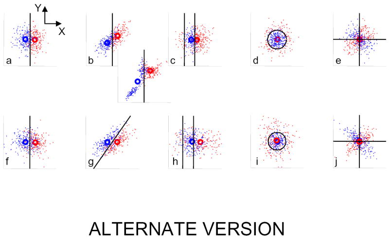
A geometric view of associations of multivariate and categorical data. In each panel, each instance of the multivariate (here, bivariate) data is represented by a point, whose coordinates X and Y are the values of its two components (e.g., pixel intensities). The color assigned to each point indicates which of the two categories is associated with it. a–e: experiments in which the multivariate quantity is the stimulus, and the categorical quantity is measured. f–j: experiments in which the multivariate quantity is measured, and the categorical quantity is the stimulus. a and f indicate the simplest situation (uncorrelated and Gaussian bivariate data, with category linearly determined by one of its components). Other panels introduce correlation structure into the bivariate data (b,g), nonlinearities (c,d,h,i), or both (e,j).

For definiteness, I will discuss the problem in terms of receptive field analysis, but the ideas apply equally well to classification image analysis. Consider an idealized (and highly simplified) receptive field mapping experiment (Fig. 2a) where the stimulus consists of uncorrelated Gaussian noise at two pixels, and the neuron responds only to one pixel. The value of the stimulus in the pixel that drives the neuron is represented by the horizontal coordinate in Fig. 2a. Since the pixel values in the stimuli are assumed to be uncorrelated, the stimuli form a circularly-symmetric cloud. The neuron is assumed to respond only to one pixel, so the probability that a point is assigned to the two response categories depends only on its horizontal position. The demarcation between “blue” responses (left half) and “red” responses (right half) is not sharp, to represent the presence of neural noise that combines additively with the stimulus.

The red and blue circles represent the results of analyzing these data by determining the average stimulus that led to each response. This is the approach taken in the standard method of reverse correlation. The horizontal displacement of these circles properly reveal a dependence of the neural response only on one pixel value. Moreover, the best partitioning of the stimuli into subsets that are associated with the two responses (based on the experimental data) is given by the perpendicular bisector of the line between these averages. This line separates the points that are closest to the center (average) of the red cloud from those that are closest to the center of the blue cloud. Thus, averaging suffices to answer two basic questions: Q_center -- what is the average stimulus corresponding to each response? and Q_rule -- what is the best way to determine which response a particular stimulus will elicit? Averaging will answer these questions when the multivariate data are independent and identically distributed, the system is linear, and noise is additive. As the next panels show, relaxation of these conditions can lead to very different results.

In cases where there is correlation between the two pixel values (Fig. 2b), averaging fails to capture the full relationship between stimulus and response. Such correlations typically are present in natural images. Even though the neuron only responds to the horizontal coordinate of the pixel, the average stimulus corresponding to each response class (circles) is now displaced along the diagonal, as a consequence of the pixel-to-pixel correlation present in the stimulus. Thus, the perpendicular bisector between the centers of the clouds, which is oblique, no longer represents the best rule for determining which response will be elicited by a given stimulus. Rather, the best rule remains a vertical line, as in Fig. 2a. In short, correlations within the stimulus set induce bias when averaging or reverse correlation is applied. This bias can be corrected if the stimulus correlations are known, and have a sufficiently simple form (for example, if the correlation is Gaussian). However, for stimulus sets such as natural stimuli, these conditions do not apply^6,7. When the correlation structure of the stimulus set is sufficiently complex, bias correction is problematic and the “average” stimulus may not be typical of any stimuli (Fig. 2b inset).

Even if the stimuli are uncorrelated, averaging will still be inadequate if the neuron is nonlinear, as the next examples show (Figs. 2c–e). Consider a neuron whose response depends only on one pixel, but this dependence has a small quadratic contribution in addition to the linear response (Fig. 2c). Because of this nonlinearity, stimuli with a large negative value at pixel X also lead to a red response. More importantly, the optimal partitioning of the stimuli into classes corresponding to the two responses (i.e., the description of what the two responses “represent”) consists of two vertical lines, not one. Averaging gives no hint of the bipartite distribution of red responses but rather misleadingly summarizes the distribution of red responses by a single point – which might even lie within the blue distribution. The latter situation would arise if the nonlinearity dominates, as would be the case in a stereotypical neuron with a symmetrical on-off response.

In another example of nonlinearity, the model neuron is an “energy” unit¹⁵ (Fig. 2d). It produces one response if X²+Y² (the energy) exceeds a criterion, and the other response if not The optimal partitioning of the stimuli into the two classes is a circle that lies on the energy threshold. Yet another example of nonlinearity is an idealized edge detector (Fig. 2e): this neuron produces one response if X and Y have opposite sign, and the other response if not – i.e., its response is determined by an interaction of the two pixel values, the product XY. In this case, the optimal rule for partitioning stimuli is described by intersecting lines that run along the axes. For both types of neuron, however, the means of the stimulus subsets that correspond to the two response classes coincide (red and blue circles in Figs, 2d,e). This means that a correlation analysis will fail to detect any signal at all, even though there is simple (but nonlinear) relationship between stimuli and response. When there is a mixture of linear and nonlinear contributions (Fig. 2c), a correlation analysis properly indicates the neuron’s dependence on input stimuli, but the signal-to-noise (i.e., the separation of the mean stimuli of each class) is less than in Fig. 2a, because of the inclusion in the average of stimuli with large negative X-values.

For the converse problem, where the stimulus is the categorical variable and the multivariate quantity is measured (i.e. optical or functional imaging), analogous situations can arise (Figs 2f–i). In the simple, ideal situation in which the stimulus activates only one pixel and there is uncorrelated, additive, Gaussian measurement noise in both pixels (Fig. 2f), the cloud of responses elicited by each stimulus is circularly symmetric, and the horizontal displacement of these clouds represents the mean response. As in Fig. 2a, the mean response to each stimulus provides an unbiased estimate of the positions of these clouds, and the perpendicular bisector between these means is the optimal partitioning of the responses into two categories.

Fig. 2g shows a situation in which a stimulus-driven response confined to one pixel adds to noise that is correlated across the two pixels – for example, by vascular pulsations. Because of this background correlation, the cloud of points that represents the pairs of pixel values corresponding to each stimulus becomes elongated and oblique. The mean image elicited by each stimulus category is no different than that of Fig. 2f. However, the optimal way to discriminate between these sets of images is no longer a vertical line: it is an oblique line, whose slope is determined by the degree of correlation of the noise background. There is a second, more subtle, effect of the fact that the sets of images elicited by each stimulus forms an elongated cloud. The oblique axis does not contribute to separation of the two clouds, but variability along it reduces the reliability of the estimates of the clouds’ centers. Thus, noise correlation has two effects: the optimal rule for discriminating the two image classes does not correspond to the perpendicular bisector of the line between their means, and a more reliable estimate of the difference between the means can be obtained by eliminating dimensions that contain large variance and small signal.

As is the case for receptive field mapping, a nonlinear relationship between the stimulus and the multivariate response makes straightforward averaging inadequate for capturing the relationship between signal and the stimulus that drove it (Figs. 2h–j). There is evidence that brain states are manifest not only by mean activity, but also by changes in power and correlation structure^16–18, suggesting that such nonlinear relationships indeed exist. These nonlinear relationships affect the mean position of each cloud of points, and the lines and curves that optimally separate the clouds, in a way similar to the analogous nonlinear relationships shown in Figs. 2c–e.

The challenges of analyzing a real dataset are substantially greater than these simple examples would suggest for several reasons. First, in a real dataset, variability would be much higher than what is illustrated in Fig. 2, so that the clouds would overlap to a much greater extent. Second, although we considered separately the effects of deviations from Gaussian uncorrelated noise (Figs. 2b,g), local nonlinearities (Figs. 2c,h), and spatial interactions (Figs. 2d,e,i,j), these phenomena are typically all present, in one degree or another. Third, the dimensionality of the multivariate dataset is typically large: 100 to 1000 in receptive field mapping or classification image experiments, 10⁵ or larger in optical or functional imaging experiments. Figure 2 considers only two-dimensional datasets. As a result, a typical dataset represents only a sparse sample of the multivariate distribution. Thus, in contrast to these examples where the dataset provides a good estimate of the shape of the distribution of the multivariate quantity, good estimates of the distribution of the multivariate quantity may not be available.

These various considerations have led to the development of sophisticated methods for analysis of such datasets. However, development of methods to deal with the effects of correlations have generally proceeded along separate lines in for receptive field mapping/classification image and imaging contexts. Attempts to analyze nonlinearities have been primarily developed for the purposes of receptive field mapping only.

Two basic questions

As highlighted in Figure 2, there are two basic questions that can be asked about the correspondence between a multivariate quantity and a categorical one: Q_center -- what is the most typical value of the multivariate quantity that corresponds to each value of the categorical variable (i.e., where is the center of each cloud)? and Q_rule -- what is the best rule for distinguishing these clouds. We do not mean to imply that the answers to these questions are the endpoints of the analysis or suffice to draw scientific conclusions, merely that they are common conceptual places to begin.

For receptive field analysis, it is natural to focus on Q_rule. Even for a neuron with very simple properties, the center of the cloud will depend on the choice of stimuli used in an experiment. But the rule, which can be thought of as a computation performed on the stimuli and an indication of what a neuronal response represents, can in principle represent a more universal characterization of the neuron.

For imaging experiments, Q_center and Q_rule are interesting and quite distinct, even if the stimulus-response relationship is linear (Fig. 2g). This is because the multivariate quantities (the pixel values) are typically highly correlated, both by the underlying physiology and the physics of imaging. The center of each cloud indeed indicates the average response to each stimulus. However, the answer to Q_rule provides additional information – how best to “read out” a pattern of activity. The distinction between the two questions cannot be avoided, because the experimenter cannot control the correlation structure of the multivariate data.

The answers to Q_center and Q_rule are usually displayed as maps – but it is important to emphasize that these maps represent very different things. For Q_center , the map is simply an instance of the multivariate quantity. But the answer to Q_rule is a rule, not an instance of the multivariate quantity. If the rule is linear, it can be rendered as a map, as follows. A linear rule is characterized as an assignment of weights (“sensitivities”) that multiply each pixel of the stimulus; the partitioning is based on a sum of these products. Thus, the map that portrays a linear rule is a map of sensitivities, i.e., quantities whose units are the reciprocal of the units of the multivariate data. Nonlinear rules can also be displayed in a map-like fashion, but here too, the map describes rules to be applied to stimuli, not stimuli themselves.

In the following sections, we consider a variety of approaches to answer Q_center and Q_rule.

Uncorrelated multivariate data

Standard analysis (subtraction of mean responses for imaging¹³, cross-correlation for receptive field^3,19 or classification image¹¹ analysis), address Q_center. As we have seen in Figure 2, Q_center and Q_rule are equivalent only under very special circumstances. When the linearity condition is relaxed but the multivariate quantity remains independent and identically distributed (Figure 2C, D, E), Q_rule can be determined by generalizations of the cross-correlation approach. The desired characterization corresponds to the “kernels” of Wiener-like^2,3,19 procedures. For example, the basic computation in the recently developed spike-triggered covariance method^4,5,8 is equivalent to the standard Lee-Schetzen cross-correlation estimate for the second-order kernel^19,20, followed by diagonalization.

In settings such as receptive field/classification image analysis, in which the investigator has control over the multivariate quantity, the use of “designer” stimulus sets (sinusoidal sums²¹ and m-sequences¹) are particularly advantageous. Such approaches are often effective in characterizing nonlinear (as well as linear) response properties. This is because these finite stimulus sets are, in some sense, more nearly uncorrelated than a random sample drawn from a large uncorrelated ensemble.

However, “designer” methods cannot be applied to imaging data, nor to situations in which natural scenes^6,7,22 or sounds^10,23 are used for receptive field determination: these multivariate stimulus sets typically contain strong correlations that cannot be controlled or fully characterized. Here, the answer to Q_rule provides information about the stimulus-response relationship that is not available from Q_center. Moreover (see below), Q_rule, along with the covariance structure of the stimulus, can provide a better estimate of Q_center than averaging.

Correlated multivariate data, linear relationship

Whether or not correlations within the high-dimensional variable are present, linear regression identifies the linear function of a stimulus sequence that does the best job (in the mean-squared sense) of predicting the binary response (spike vs. no spike; target seen vs. target not seen). Thus, it is a natural approach to finding Q_rule under the assumption that the stimulus-response relationship is linear, and it can be extended in a Wiener-like fashion to nonlinear relationships, as has been done in the context of receptive field analysis²⁴. Of note, linear regression was used in the original description of the classification image method¹². Other than a few exceptions²⁵, this approach is not often taken because there are statistical difficulties that confound direct application of linear regression to the experimental contexts we are considering. However, as we next describe, there are recently developed techniques that can surmount these difficulties.

In essence, finding Q_rule via linear regression requires two steps (see Appendix): (i) estimating the covariance matrix S of the multivariate set, and (ii) multiplication of the mean difference between the two multivariate clouds by S⁻¹, the matrix inverse of S. The covariance matrix S is a symmetric array, whose entires s_jk are the correlations of the jth and kth pixels. For independent identically distributed data, S is proportional to the identity matrix, and linear regression reduces to simple subtraction, since S⁻¹ is also proportional to the identity. In imaging data, pixel values are coupled by motion, light scatter, blood flow, and other physiologic factors; in receptive field analysis, pixel values are coupled by the statistics of natural scenes^23,26. Thus, linear regression and the related approaches described below differ fundamentally from the subtraction method, since S is far from the identity matrix.

The main pitfall in linear regression is that of overfitting – namely, the estimated answer to Q_rule may work well for the particular experimental sampling of the multivariate dataset, but does not generalize to a larger sample. Linear regression only provides an answer to Q_rule that generalizes if the correlation structure of the multivariate data is well-characterized by the experimental sample. This characterization requires enough samples to estimate its covariance matrix S, along with an assumption, typically Gaussianity, to determine higher-order correlations from second-order correlations. For optical or functional imaging data, there are typically many more pixels (10⁵ to 10⁶) than samples (ca. 10⁴). For receptive field/classification image data, the undersampling problem is present but less severe (10³ to 10⁴ pixels; number of samples in the same range), but the correlation structure (especially of natural images) is likely to be very non-Gaussian. Because of undersampling and/or non-Gaussian characteristics of the multivariate data, direct application of standard linear regression is likely to produce results that are worse than simple subtraction.

However, extensions of linear regression^27–29 developed for imaging are applicable to the undersampled regime, by recasting the problem in a form that does not require explicit inversion of S. These approaches focus on the eigenvectors of the covariance matrix S and related matrices (see Appendix). The eigenvectors of S (which are its “principal components”) are a small set of images, from which all images can be reconstructed. Eigenvectors can be ranked in importance according to their eigenvalue. The larger the eigenvalue corresponding to an eigenvector, the greater the extent to which the stimulus set explores the corresponding image direction. Based on the eigenvalues, one can select a subset of eigenvectors, within which an linear regression-like like procedure can be carried out accurately. In the example of Figure 2g, such a procedure would correspond to restricting the estimation process to the direction that crosses the narrow axes of the ellipse, and forgoing an attempt to estimate the position of the ellipse centers along their long axes, where variability is greater.

As detailed in the Appendix, there are several useful variations on this theme. The “truncated inverse” method²⁸ selects the eigenvectors of S whose eigenvalues are sufficiently large. More elaborate approaches select a subspace based not only on the overall covariance structure of S but also on the covariances within the subset of stimuli that lead to each categorical response. This includes the classic Fisher²⁷ discriminant method, which restricts analysis to the one-dimensional projection that optimally discriminates between Gaussian fits to the two clouds. The “indicator function” method³⁰ projects into several dimensions (the “canonical variates”), chosen on the basis of a significance criterion. Canonical variates are also the basis of a method for characterizing spatiotemporal aspects of images acquired in fast fMRI studies^31,32. A further variation is the “generalized indicator function method”²⁹, that considers the eigenvectors of a linear mix of S and the within-group covariances, and weights these eigenvectors in a graded fashion (see Appendix).

These approaches all represent methods of dimensionality reduction –selection of subspaces that are likely to contain a large signal-to-noise ratio (SNR). Within this general framework, independent components analysis³³ can be viewed as a strategy for using higher moments of the images to identify mixtures of subspaces that are likely to contain signal³⁴. There are other approaches to enhance SNR in functional imaging data that exploit specific features of such images (e.g., vascular artifacts³⁵), but since these approaches are domain-specific, we do not discuss them here.

Dimensional reduction can also be viewed as a form of “regularization”^36–38 to avoid the pitfalls of estimating this covariance structure from very limited data. The generalized indicator function method²⁹ can be viewed as a regularized determination of canonical variates^37,38. “Ridge regression”³⁸ (see Appendix) is a regularization strategy (widely applied outside of neuroscience) that chooses a compromise between the estimated covariance matrix and the identity matrix. Variations of ridge regression that take into account smoothness constraints have recently been used to extract receptive field maps from natural stimuli, both in the visual²² and auditory¹⁰ domains, but apparently have not been applied in optical or functional imaging.

Correlated multivariate data, nonlinear relationship

In functional imaging, analytical methods (including the recent developments reviewed above) assume that the relationship between the imaged signal and neural activity is linear³⁹, and the analytical focus has been on determining this relationship when the activity-dependent signal represents a very small fraction of the image. In receptive field analysis, it is generally considered that the neural response will be substantially greater than background when the stimulus is appropriate, but it is recognized that the stimulus-response relationship may not be linear^6,40. This has driven the development of efficient methods for identifying nonlinear relationships that succeed even in the presence of strongly non-Gaussian multivariate data^6,40. Moreover, the neural response, even if considered categorical, is generated in a manner that has stochastic and dynamic aspects. Understanding the implications of spike generation for the convergence and bias credentials of various estimation techniques⁴⁰, and the interpretation of the resulting receptive fields^41,42 is another focus of current work.

Time for a convergence?

One can readily identify several reasons for the separate development of analytical techniques in receptive field/classification image analysis and optical/functional imaging, owing to various differences between these settings. However, we argue that the implications of these differences are less compelling than generally assumed, and consequently, that there are likely to be substantial opportunities for synergy.

Most obviously (Fig. 1), the categorical and multivariate characteristics of stimulus and response are swapped. This has two implications. If the experimenter is willing to choose a “designer” stimulus set, then there are opportunities for improved experimental design in receptive field or classification image analysis that are not available for optical or functional imaging – but we do not focus on these here, and these are irrelevant to receptive field/classification image studies using natural stimuli. The other implication is that this distinction leads to a difference in how noise is considered. In imaging, no threshold is typically postulated; rather, neuronal and measurement variability smoothly combine with the “signal.” For receptive field and classification image analysis, it is generally assumed that after a computation is performed on the multivariate quantity, there is a threshold (e.g., a firing threshold, or a decision threshold), which may in part be stochastic. However, many treatments seek a rule for the firing rate (or decision variable) that minimizes the mean-squared prediction error, rather than an explicit maximum-likelihood solution for a model with a threshold. Since mean-squared error criterion is essentially a maximum-likelihood criterion for an assumed Gaussian noise, it is tantamount to ignoring the statistical consequences of the threshold.

Consequently, unless detailed dynamics of spike trains are of interest, the stimulus-response inversion does not prevent application of analysis methods for receptive field mapping to imaging, and vice-versa. Explicit modeling of spike train dynamics may result in further improvement and insight^40–42. But dynamics (i.e., the effect of stimulus sequence and timecourse on response) are also present in an optical or functional experiment, suggesting that techniques to examine dynamics developed for receptive field analysis might usefully be applied to imaging.

Another apparent difference between these settings is what is typically considered limiting: in classification image experiments, the number of trials that can be obtained may be limited to 10³ to 10⁴, since each trial requires an explicit behavioral response. In imaging, the main hurdle to analysis is usually considered to be an intrinsically low SNR: 1 in 10³ to 1 in 10⁴ for optical imaging, 1 in 10² for fMRI. There may also be sources of variability that lead to highly structured artifacts, such as pulsatile movements of the tissue. Since receptive field studies often have the implicit goal of prediction of responses to stimuli outside of the experimental sample, undersampling of the stimulus space is often considered to be the main problem, since (even when the SNR is high), a far greater sampling is required to construct a nonlinear model than to construct a linear model. However, SNR, number of trials, and sampling of the stimulus space are always limiting. Analytical approaches that make better use of a given data set to identify smaller signals, provide greater spatial detail, or shorten the experiment time to obtain results of a given quality are always useful, especially given the increasing availability of computational resources and the costs (not just direct economic) of obtaining neurophysiologic data. Moreover, approaches to imaging data analysis in the presence of structured noise is closely analogous to identification of receptive fields from “natural” stimulus sets⁶, which have strong but incompletely determined statistical structure.

In optical and functional imaging, the relationship of the multivariate quantity to a behavioral index is typically assumed to be linear³⁹, while a linear relationship is not always assumed in classification image analysis^43,44 and in receptive field mapping^2,3. But there is increasing recognition^16–18 that stimulus-induced changes in the correlation structure of brain activity measures, and not just its mean level, are behaviorally and mechanistically relevant. Identifying such changes in imaging data is closely allied with identifying nonlinear aspects of a neural stimulus-response relationship in the receptive field mapping context.

Even for imaging studies that do not seek a nonlinear relationship between stimuli and the imaging data, inclusion of a nonlinearity in the model might nevertheless benefit the goal of signal extraction – i.e., identifying the rule that distinguishes responses to the members of the stimulus set. An analytic procedure that forces a nonlinear relationship to be modeled as a linear one necessarily causes some “signal” (the deviation of a systematic nonlinear response from a linear one) to appear as “noise”. Application of traditional nonlinear kernel methods is problematic, since the introduction of a large number of free parameters would likely defeat any benefit of capturing more signal. However, it would be very worthwhile to explore the use of recent receptive field mapping methods that seek simple nonlinear relationships in an efficient manner^6,40. It should be emphasized that even if the relationship between the imaging signal and neural activity were strictly linear³⁹, one would still expect this approach to be of value. Such linearity applies to the mean signal, not its fluctuations – and the in the noisy, multivariate regime, the latter may dominate the stimulus-response relationship. Moreover, mean neural activity may not be linearly related to the categorical variable –an issue that becomes relevant in experiments in which the categorical variable can take on more than two values, such as an orientation or spatial frequency experiment.

Conversely, to maximize the ability to test mechanistic or functional receptive field models, it is necessary to identify not only the large readily-resolvable components, but small contributions as well – as illustrated by the recent analysis of complex cell receptive fields in terms of spike-triggered covariances^5,8. Moreover, it is evident that further insight into neuronal properties can be gleaned from receptive field characterization with stimulus sets have complex statistics, including natural scenes^6,7,23. For both of these reasons, analytical methods developed for imaging that improve signal to noise by using subspace selection³⁸ may be useful. One might even envision that such methods could be further refined (for receptive field characterization) by guiding the estimation of covariances by the known statistical regularities of natural images^26,45,46.

Conclusion

As detailed above, the problem of identifying the relationship between a highly multivariate quantity and a categorical quantity (such as a discrete stimulus, a behavioral response, or the presence of an action potential) is deceptively simple. It has been approached by a variety of analytical techniques, most often motivated by particular features of one of these contexts. We claim that the distinctions between experimental domains are not as deep as generally assumed, and speculate that opportunities for progress will result from applying these techniques (or, the ideas behind them) beyond their original domain.

The above considerations are only starting points, not an exhaustive list, and it is likely that the benefits will be relatively specific to particular experimental situations and goals. Whether cross-application of such methods and ideas will result in new qualitative insights, or merely incremental advances, is difficult to predict. Nevertheless, recognition of the close relationships between the mathematical challenges in these domains will enrich and accelerate the development of improved analytical techniques.

Appendix

We briefly summarize some of the data analysis methods mentioned in the text. We denote the two values of the categorical variable (e.g., two stimulus classes in optical and functional imaging, or two response classes in receptive field or classification mapping) by the labels 0 and 1. An instance of the multivariate quantity (an “image”) is denoted by a row vector x, consisting of P pixel values. We assume that class j (j=0 or 1) is associated with N_j observations of x; the kth observation is a row vector x_k^[j]. With these conventions, the within-class mean for class j is given by the row vector ${\mu }_j=\frac{1}{N_j}\sum _{k=1}^{N_j}{x}_k^{[j]}$ and the global mean is $\mu =\frac{N_0{\mu }_0+N_1{\mu }_1}{N_0+N_1}$.

The difference image is the row vector v_DI = μ₁ − μ₀.

Formally, linear regression, the Fisher discriminant, and their extensions seek specific linear functions on images (that is, a rule to be applied to images), not images per se. Operation of a linear function f on an image x can be regarded as the matrix product xf of the row vector x and the column vector f. A column vector f can be regarded as a transpose of a row (image) vector, f = v^T.

The linear regression method seeks a linear function f_LR on the set of images that provides the best prediction of the response (0 or 1). f_LR = v^T_LR, wherev_LR is the row (image) vector that minimizes $\sum _{j=0}^1\sum _{k=1}^{N_j}{\left|(x_k^{[j]}-\gamma )v_{LR}{}^T-j\right|}^2$.

f_LR = v^T_LR may be calculated from the covariance matrix, $S=\sum _{j=0}^1\sum _{k=1}^{N_j}{(x_k^{[j]}-\mu )}^T(x_k^{[j]}-\mu ).$

Provided that the covariance matrix S is invertible, $f_{LR}=\frac{N_0{N}_1}{N_0+N_1}{S}^{-1}{({\mu }_1-{\mu }_0)}^T$. If the covariance matrix is not invertible, v_LR is not unique.

The truncated difference method ²⁸restricts the LR estimate to the subspace spanned by the eigenvectors of S whose eigenvalues are within some range λ_min < λ < λ_max. (For a symmetric matrix M, a column vector c is said to be an eigenvector of M if Mc = αc for some scalar α, and α s said to be the eigenvalue corresponding to c).

Ridge regression ³⁸adds a multiple of the identity to S, i.e., replaces S by S + κI above. Other regularization procedures replace S by S + κI + ρC , where nonzero elements of C reflect penalties for a lack of smoothness in the estimated image ν. Here, κ and ρ are scalars, typically chosen by optimizing the ability of a model based on ν to predict stimulus-response relationships in a separate dataset.

The canonical variates are the solutions of the generalized eigenvalue problem (μ₁ − μ₀)^T (μ₁ − μ₀) f = λ(S₀ + S₁) f, where S₀ and S₁ are the within-class covariance matrices, $S_j=\sum _{k=1}^{N_j}{(x_k^{[j]}-{\mu }_j)}^T(x_k^{[j]}-{\mu }_j).$

The Fisher discriminant ²⁷is the linear function f_FD on the set of images that best discriminates between the images that correspond to the two response classes. That is, f_FD maximizes the ratio of the projected difference between classes, ${\left|({\mu }_1-{\mu }_0)f_{FD}\right|}^2,$ to the projected variances within classes, $\sum _{j=0}^1\sum _{k=1}^{N_j}{\left|(x_k^{[j]}-{\mu }_j)f_{FD}\right|}^2.$ For Gaussian data, this maximum is achieved when f_FD is the eigenvector corresponding to the largest eigenvalue of the above generalized eigenvalue problem. Method I of the indicator function method ³⁰is essentially the Fisher discriminant. Method II considers multiple eigenvectors, whose eigenvalues are sufficiently large. The generalized indicator function method ²⁹considers eigenvectors of the more general operator (μ₁ − μ₀)^T (μ₁ − μ₀) − α(S₀ + S₁) for some “quality control” parameter α, adds a regularization term, and applies additional criteria to select and weight these eigenvectors.

References

- 1.Sutter E. Nonlinear Vision:Determination of Neural Receptive Fields, Function, and Networks. In: Pinter R, Nabet B, editors. CRC Press; Cleveland: 1992. pp. 171–220. [Google Scholar]
- 2.Chichilnisky EJ. A simple white noise analysis of neuronal light responses. Network. 2001;12:199–213. [PubMed] [Google Scholar]
- 3.Marmarelis PZ, Naka K. White-noise analysis of a neuron chain: an application of the Wiener theory. Science. 1972;175:1276–8. doi: 10.1126/science.175.4027.1276. [DOI] [PubMed] [Google Scholar]
- 4.Simoncelli E, Paninski L, Pillow J, Schwartz O. The Cognitive Neurosciences. In: Gazzaniga M, editor. 3rd Edition. MIT Press; Cambridge, MA: 2004. [Google Scholar]
- 5.Touryan J, Lau B, Dan Y. Isolation of relevant visual features from random stimuli for cortical complex cells. J Neurosci. 2002;22:10811–8. doi: 10.1523/JNEUROSCI.22-24-10811.2002. [DOI] [PMC free article] [PubMed] [Google Scholar]
- 6.Sharpee T, Rust NC, Bialek W. Analyzing neural responses to natural signals: maximally informative dimensions. Neural Comput. 2004;16:223–50. doi: 10.1162/089976604322742010. [DOI] [PubMed] [Google Scholar]
- 7.David SV, Vinje WE, Gallant JL. Natural stimulus statistics alter the receptive field structure of v1 neurons. J Neurosci. 2004;24:6991–7006. doi: 10.1523/JNEUROSCI.1422-04.2004. [DOI] [PMC free article] [PubMed] [Google Scholar]
- 8.Rust NC, Schwartz O, Movshon JA, Simoncelli EP. Spatiotemporal elements of macaque v1 receptive fields. Neuron. 2005;46:945–56. doi: 10.1016/j.neuron.2005.05.021. [DOI] [PubMed] [Google Scholar]
- 9.Escabi MA, Schreiner CE. Nonlinear spectrotemporal sound analysis by neurons in the auditory midbrain. J Neurosci. 2002;22:4114–31. doi: 10.1523/JNEUROSCI.22-10-04114.2002. [DOI] [PMC free article] [PubMed] [Google Scholar]
- 10.Machens CK, Wehr MS, Zador AM. Linearity of cortical receptive fields measured with natural sounds. J Neurosci. 2004;24:1089–100. doi: 10.1523/JNEUROSCI.4445-03.2004. [DOI] [PMC free article] [PubMed] [Google Scholar]
- 11.Eckstein MP, Ahumada AJ., Jr Classification images: a tool to analyze visual strategies. J Vis. 2002;2:1x. doi: 10.1167/2.1.i. [DOI] [PubMed] [Google Scholar]
- 12.Ahumada AJ, Jr, Lovell J. Stimulus features in signal detection. Journal of the Acoustical Society of America. 1971;49:1751–1756. [Google Scholar]
- 13.Grinvald A. Optical imaging of architecture and function in the living brain sheds new light on cortical mechanisms underlying visual perception. Brain Topogr. 1992;5:71–5. doi: 10.1007/BF01129033. [DOI] [PubMed] [Google Scholar]
- 14.Kwong KK, et al. Dynamic magnetic resonance imaging of human brain activity during primary sensory stimulation. Proc Natl Acad Sci U S A. 1992;89:5675–9. doi: 10.1073/pnas.89.12.5675. [DOI] [PMC free article] [PubMed] [Google Scholar]
- 15.Ohzawa I, DeAngelis GC, Freeman RD. Encoding of binocular disparity by complex cells in the cat's visual cortex. J Neurophysiol. 1997;77:2879–909. doi: 10.1152/jn.1997.77.6.2879. [DOI] [PubMed] [Google Scholar]
- 16.Pesaran B, Pezaris JS, Sahani M, Mitra PP, Andersen RA. Temporal structure in neuronal activity during working memory in macaque parietal cortex. Nat Neurosci. 2002;5:805–11. doi: 10.1038/nn890. [DOI] [PubMed] [Google Scholar]
- 17.Kenet T, Bibitchkov D, Tsodyks M, Grinvald A, Arieli A. Spontaneously emerging cortical representations of visual attributes. Nature. 2003;425:954–6. doi: 10.1038/nature02078. [DOI] [PubMed] [Google Scholar]
- 18.Rodriguez E, et al. Perception's shadow: long-distance synchronization of human brain activity. Nature. 1999;397:430–3. doi: 10.1038/17120. [DOI] [PubMed] [Google Scholar]
- 19.Lee Y, Schetzen M. Measurement of the kernels of a nonlinear system by cross-correlation. Int J Control. 1965;2:237–254. [Google Scholar]
- 20.Bialek W, de Ruyter van Steveninck R. Real-time performance of a movement sensitive neuron in the blowfly visual system: coding and information transfer in short spike sequences. Proc Roy Soc Lond B. 1988;234:379–414. [Google Scholar]
- 21.Victor JD, Shapley RM, Knight BW. Nonlinear analysis of cat retinal ganglion cells in the frequency domain. Proc Natl Acad Sci U S A. 1977;74:3068–72. doi: 10.1073/pnas.74.7.3068. [DOI] [PMC free article] [PubMed] [Google Scholar]
- 22.Smyth D, Willmore B, Baker GE, Thompson ID, Tolhurst DJ. The receptive-field organization of simple cells in primary visual cortex of ferrets under natural scene stimulation. J Neurosci. 2003;23:4746–59. doi: 10.1523/JNEUROSCI.23-11-04746.2003. [DOI] [PMC free article] [PubMed] [Google Scholar]
- 23.Theunissen FE, et al. Estimating spatio-temporal receptive fields of auditory and visual neurons from their responses to natural stimuli. Network. 2001;12:289–316. [PubMed] [Google Scholar]
- 24.Korenberg MJ, Bruder SB, McIlroy PJ. Exact orthogonal kernel estimation from finite data records: extending Wiener's identification of nonlinear systems. Ann Biomed Eng. 1988;16:201–14. doi: 10.1007/BF02364581. [DOI] [PubMed] [Google Scholar]
- 25.Levi DM, Klein SA. Classification images for detection and position discrimination in the fovea and parafovea. J Vis. 2002;2:46–65. doi: 10.1167/2.1.4. [DOI] [PubMed] [Google Scholar]
- 26.Simoncelli EP, Olshausen BA. Natural image statistics and neural representation. Annu Rev Neurosci. 2001;24:1193–216. doi: 10.1146/annurev.neuro.24.1.1193. [DOI] [PubMed] [Google Scholar]
- 27.Fisher RA. The use of multiple measurements in taxonomic problems. Annals of Eugenics. 1936;7:179–188. [Google Scholar]
- 28.Gabbay M, Brennan C, Kaplan E, Sirovich L. A principal components-based method for the detection of neuronal activity maps: application to optical imaging. Neuroimage. 2000;11:313–25. doi: 10.1006/nimg.2000.0547. [DOI] [PubMed] [Google Scholar]
- 29.Yokoo T, Knight BW, Sirovich L. An optimization approach to signal extraction from noisy multivariate data. Neuroimage. 2001;14:1309–26. doi: 10.1006/nimg.2001.0950. [DOI] [PubMed] [Google Scholar]
- 30.Everson R, Knight BW, Sirovich L. Separating spatially distributed response to stimulation from background. I. Optical imaging. Biol Cybern. 1997;77:407–17. doi: 10.1007/s004220050400. [DOI] [PubMed] [Google Scholar]
- 31.Friston KJ, Frith CD, Frackowiak RS, Turner R. Characterizing dynamic brain responses with fMRI: a multivariate approach. Neuroimage. 1995;2:166–72. doi: 10.1006/nimg.1995.1019. [DOI] [PubMed] [Google Scholar]
- 32.Worsley KJ, Poline JB, Friston KJ, Evans AC. Characterizing the response of PET and fMRI data using multivariate linear models. Neuroimage. 1997;6:305–19. doi: 10.1006/nimg.1997.0294. [DOI] [PubMed] [Google Scholar]
- 33.Bell AJ, Sejnowski TJ. An information-maximization approach to blind separation and blind deconvolution. Neural Comput. 1995;7:1129–59. doi: 10.1162/neco.1995.7.6.1129. [DOI] [PubMed] [Google Scholar]
- 34.Thomas CG, Harshman RA, Menon RS. Noise reduction in BOLD-based fMRI using component analysis. Neuroimage. 2002;17:1521–37. doi: 10.1006/nimg.2002.1200. [DOI] [PubMed] [Google Scholar]
- 35.Carmona RA, Hwang WL, Frostig RD. Wavelet analysis for brain function imaging. IEEE Trans on Medical Imaging. 1995;14:556–564. doi: 10.1109/42.414621. [DOI] [PubMed] [Google Scholar]
- 36.Tikhonov AN, Arsenin VY. Wiley, Hoboken; NJ: 1977. Solutions of ill-posed problems. [Google Scholar]
- 37.Hastie T, Buja A, Tibshirani R. Penalized discriminant analysis. Annals of Statistics. 1995;23:73–102. [Google Scholar]
- 38.Hastie T, Tibshirani R, Friedman J. Springer-Verlag; New York: 2001. The elements of statistical learning: data mining, Inference, and prediction. [Google Scholar]
- 39.Boynton GM, Engel SA, Glover GH, Heeger DJ. Linear systems analysis of functional magnetic resonance imaging in human V1. J Neurosci. 1996;16:4207–21. doi: 10.1523/JNEUROSCI.16-13-04207.1996. [DOI] [PMC free article] [PubMed] [Google Scholar]
- 40.Paninski L. Convergence properties of three spike-triggered analysis techniques. Network. 2003;14:437–64. [PubMed] [Google Scholar]
- 41.Aguera y Arcas B, Fairhall AL. What causes a neuron to spike? Neural Comput. 2003;15:1789–807. doi: 10.1162/08997660360675044. [DOI] [PubMed] [Google Scholar]
- 42.Pillow J, Simoncelli E. Biases in white noise analysis due to non-Poisson spike generation. Neurocomputing. 2003;52:109–115. [Google Scholar]
- 43.Neri P. Estimation of nonlinear psychophysical kernels. J Vis. 2004;4:82–91. doi: 10.1167/4.2.2. [DOI] [PubMed] [Google Scholar]
- 44.Neri P, Heeger DJ. Spatiotemporal mechanisms for detecting and identifying image features in human vision. Nat Neurosci. 2002;5:812–6. doi: 10.1038/nn886. [DOI] [PubMed] [Google Scholar]
- 45.Field DJ. Relations between the statistics of natural images and the response properties of cortical cells. J Opt Soc Am [A] 1987;4:2379–94. doi: 10.1364/josaa.4.002379. [DOI] [PubMed] [Google Scholar]
- 46.Dong DW, Atick JJ. Statistics of natural time-varying images. Network-Computation in Neural Systems. 1995;6:345–358. [Google Scholar]
Associated Data
This section collects any data citations, data availability statements, or supplementary materials included in this article.