

Abstract
Background
The potential public health benefits of targeting environmental interventions by genotype depend on the environmental and genetic contributions to the variance of common diseases, and the magnitude of any gene-environment interaction. In the absence of prior knowledge of all risk factors, twin, family and environmental data may help to define the potential limits of these benefits in a given population. However, a general methodology to analyze twin data is required because of the potential importance of gene-gene interactions (epistasis), gene-environment interactions, and conditions that break the 'equal environments' assumption for monozygotic and dizygotic twins.
Method
A new model for gene-gene and gene-environment interactions is developed that abandons the assumptions of the classical twin study, including Fisher's (1918) assumption that genes act as risk factors for common traits in a manner necessarily dominated by an additive polygenic term. Provided there are no confounders, the model can be used to implement a top-down approach to quantifying the potential utility of genetic prediction and prevention, using twin, family and environmental data. The results describe a solution space for each disease or trait, which may or may not include the classical twin study result. Each point in the solution space corresponds to a different model of genotypic risk and gene-environment interaction.
Conclusion
The results show that the potential for reducing the incidence of common diseases using environmental interventions targeted by genotype may be limited, except in special cases. The model also confirms that the importance of an individual's genotype in determining their risk of complex diseases tends to be exaggerated by the classical twin studies method, owing to the 'equal environments' assumption and the assumption of no gene-environment interaction. In addition, if phenotypes are genetically robust, because of epistasis, a largely environmental explanation for shared sibling risk is plausible, even if the classical heritability is high. The results therefore highlight the possibility – previously rejected on the basis of twin study results – that inherited genetic variants are important in determining risk only for the relatively rare familial forms of diseases such as breast cancer. If so, genetic models of familial aggregation may be incorrect and the hunt for additional susceptibility genes could be largely fruitless.
Background
Some geneticists have predicted a genetic revolution in healthcare: involving a future in which individuals take a battery of genetic tests, at birth or later in life, to determine their individual 'genetic susceptibility' to disease [1,2]. In theory, once the risk of particular combinations of genotype and environmental exposure is known, medical interventions (including lifestyle advice, screening or medication) could then be targeted at high-risk groups or individuals, with the aim of preventing disease [3].
However, there are also many critics of this strategy, who argue that it is likely to be of limited benefit to health [4-8]. One area of debate concerns the proportion of cases of a given common disease that might be avoided by targeting environmental or lifestyle interventions to those at high genotypic risk. Known genetic risk factors have to date shown limited utility in this respect [9]. However, some argue that combinations of multiple genetic risk factors may prove more useful in the future [10].
There are two possible approaches to considering this issue. The 'bottom-up' approach seeks to identify individual genetic and environmental risk factors and their interactions and quantify the risks. However, this approach is limited by the difficulties in establishing the statistical validity of genetic association studies and of quantifying gene-gene and gene-environment interactions: see, for example, [11-14].
A 'top-down' approach instead considers risks at the population level using twin and family studies and data on the importance of environmental factors in determining a trait. However, analysis of twin data is usually limited by the assumptions made in the classical twin study [15], including that: (i) there are no gene-gene interactions (epistasis); (ii) there are no gene-environment interactions; (iii) the effects of environmental factors shared by twins are independent of zygosity (the 'equal environments' assumption). These assumptions have all been individually explored and shown to be important in influencing the conclusions drawn from twin and family data [16-18]. In addition, the magnitude of any gene-environment interaction is critically important in determining the utility of targeting environmental interventions by genotype [19]. Although a general methodology to analyze twin data without making these assumptions has been developed, the algebra becomes intractable once multiple loci are involved [17]. This is problematic because, for common diseases, the impacts of multiple genetic variants, and potentially the whole genetic sequence, on disease susceptibility (here called 'genotypic risk') may be important.
The four-category model of population risks developed by Khoury and others [19] is a useful starting point for a top-down analysis of genetic prediction and prevention. It allows the merits of a targeted intervention strategy (which seeks to reduce the exposure of the high-risk genotype group only) to be explored, and can readily be extended to include more than four risk categories [10]. However, this model's use to date has been limited to bottom-up consideration of single genetic variants or to studying hypothetical examples of multiple variants. The four-category model is limited by the assumption of no confounders, which means it is applicable to only a subset of possible models of gene-gene and gene-environment interaction. However, situations where the 'no confounders' assumption is valid are arguably most likely to be of relevance to public health.
The aim of this paper is to combine the four-category model with population level data from twin, family and environmental studies, without adopting the classical twin model assumptions. This model of gene-gene and gene-environment interactions is then used to implement a 'top-down' approach to quantifying the utility of genetic 'prediction and prevention'.
Method
The four-category model
Consider a population divided into genotypic or environmental risk categories for a given trait (Figure 1a and 1b). The fraction of the population in the 'high environmental risk group' (designated by subscript e) is ε, and this subpopulation is at risk re. The remainder of the population is at risk roe. The fraction of the population in the 'high genotypic risk' group (designated by the subscript g) is γ, and this subpopulation is at risk rg, with the remainder of the population at risk rog. The total risk rt for this trait in this population is then given by:
Figure 1.
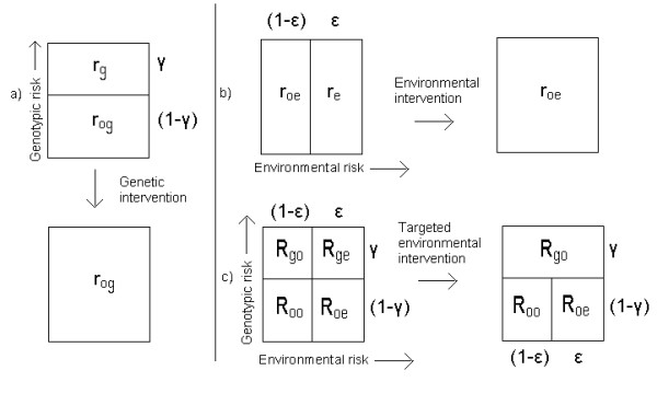
The four-category model. A population divided into: (a) high and low genotypic risk categories (rg and rog); (b) high and low environmental risk categories (re and roe); (c) four categories based on combined genotypic and environmental risk.
rt = γrg + (1-γ)rog (1)
or by:
rt = εre + (1-ε)roe (2)
The same population can alternatively be divided into four categories, making a four-category model (Figure 1c)) with risks Roo, Roe, Rgo and Rge. Table 1 shows the risk categories in this model.
Table 1.
The four category model: risks and cases for a population of size N.
| Category | Risk of being in category | Number of people in category | Number of cases in category |
| ge (high-risk genotype/high-risk exposure) | Rge | γεN | γε RgeN |
| go (high-risk genotype/low-risk exposure) | Rgo | γ (1-ε)N | γ (1-ε)RgoN |
| oe (low-risk genotype/high-risk exposure) | Roe | ε (1-γ)N | ε (1-γ)RoeN |
| oo (low-risk genotype/low-risk exposure) | Roo | (1-ε) (1-γ)N | (1-ε) (1-γ)RooN |
| Total | N | rtN | |
The risks are related to the previous definitions by:
rg = εRge + (1-ε) Rgo (3)
rog = εRoe + (1-ε) Roo (4)
re = γRge + (1-γ) Roe (5)
roe = γRog + (1-γ) Roo (6)
The category risks R remain constant in different populations (i.e. as ε and γ vary), provided there are no confounders. This assumption restricts the model to special cases of gene-gene and gene-environment interaction. Note that for a single genetic variant, rg corresponds to the penetrance of the variant, and that in general (provided Rge ≠ Rgo) this varies with the proportion of the population in the high exposure group, ε, as has been observed [20,21].
The total risk for the given trait is given by:
rt = γεRge + γ(1-ε)Rgo + ε(1-γ)Roe + (1-ε)(1-γ)Roo (7)
The subpopulation of cases has different characteristics from the general population: for example, it contains a higher proportion of people from the 'ge' subgroup. The relative risk for a person drawn randomly from a subpopulation with the same genotypic and environmental characteristics as the cases, RRcases, is given by the sum of the relative risks for each category shown in Table 1:
Similarly, the relative risk for a person drawn randomly from a subpopulation with the same genotypic characteristics as the cases (but with the environmental characteristics of the general population) is:
The relative risk for a person drawn randomly from a subpopulation with the same environmental characteristics as the cases (but with the genotypic characteristics of the general population) is:
Population attributable fractions
Provided there are no confounders, the population attributable fraction (PAFEe) due to the presence of the high exposure (E) in the high exposure population subgroup (e) may be defined as:
If the trait is a disease, PAFEe is the proportion of cases that could be avoided if an environmental intervention (such as a lifestyle change or reduction in exposure) succeeds in moving everyone in the 'high environmental risk group' to the 'low environmental risk' category, as shown in Figure 1b.
The targeted population attributable fraction (PAFEge) may be defined as the proportion of cases that could be avoided by targeting the same environmental intervention at the 'high genotypic + high environmental risk' subgroup only (the 'ge' subgroup), as shown in Figure 1c. Again assuming no confounders, it is given by:
Note that PAFEge differs from PAFge as defined by Khoury & Wagener [19]. The latter implicitly assumes that both environmental and genetic risk factors are reduced and thus is inappropriate for assessing the merits of a targeted environmental intervention. PAFEge as defined here is instead equivalent to the targeted attributable fraction (AFT) defined by Khoury et al. [10]. To avoid confusion, the notation adopted here specifies both the nature of the intervention (environmental, denoted by superscript E) and the target subpopulation (the 'ge' subgroup, at both high genotypic and high environmental risk). Thus, the proportion of cases that would be avoided were it possible to move the 'high genotypic risk' subgroup to 'low genotypic risk' (as shown in Figure 1a) is written as PAFGg, given by:
Although in practice it is not possible to change the genotype of the population, the parameter PAFGg is nevertheless useful in the calculations that follow.
Measures of utility
Khoury et al. [10] define the Population Impact (PI) as:
PI is one possible measure of the usefulness of targeting the environmental intervention (E) at the 'ge' subgroup. It measures the proportion of cases avoided by targeting the 'high genotypic + high environmental risk' subgroup (the 'ge' subgroup), compared to the proportion avoided by applying the environmental intervention to the whole 'high environmental risk' group. PI has the property:
0 ≤ PI ≤ 1 (15)
and has its maximum value when PAFEge = PAFEe. However, as a measure of the utility of genotyping, PI has the disadvantage that it takes no account of the proportion of the population γ in the high genotypic risk group. This means PI = 1 when γ = 1 simply because the whole population is then in the high genotypic risk group, although using genotyping to target environmental interventions is more likely to be useful if PI = 1 and γ is also small.
Therefore, consider an alternative utility parameter Uge, defined by:
which has the property
-γ ≤ Uge ≤ (1-γ) (17)
Uge tends to 1 only if PI = 1 and γ is also small. It is a measure of the utility of using genotyping to target the environmental intervention at the 'ge' subgroup, compared to randomly selecting the same proportion γ of the population to receive the intervention. Uge is positive if those at high genotypic risk have more to gain than those at low genotypic risk from the intervention ((Rge-Rgo) ≥ (Roe-Roo)) and negative if they have less to gain from the intervention. This reflects the fact that targeting those who have least to gain through an intervention is worse than using random selection in terms of its impact on population health.
Note that even if genotyping is better than random selection, other types of test that are more useful may be available [22]; a population-based approach still has the potential to reduce more cases of disease [9,19,23]; and such targeting also has broader psychological and social implications. Therefore a positive Uge does not necessarily imply that genotyping is the best means of selecting a subpopulation to target, or that a targeted approach is necessarily effective or socially acceptable. Note also that the measure Uge applies only to interventions that are considered applicable to the whole population (such as smoking cessation) and neglects other relevant issues such as cost-effectiveness and the burden of disease [24]. In addition, it is necessary to consider the magnitude of the Population Attributable Fraction, PAFEe before proposing this approach. This is because both PI and Uge may tend to unity even if only a small proportion of cases can be avoided by means of environmental interventions.
Limits on parameters
Consider only populations where rg ≥ rog and re ≥ roe for all values of ε and γ. Then the risks in the four box model must be ordered such that:
1 ≥ Rge ≥ Roe ≥ Roo ≥ 0 (18)
and
Rge ≥ Rgo ≥ Roo (19)
Using the known relationships (Equations (11), (13) and (16)) between PAFEe, PAFGg, Uge and the risks Roo, Rgo, Roe and Rge, leads to the limits on the utility parameter Uge shown in Table 2. These conditions also ensure that PAFEe, PAFGg and PAFEge are all positive. The two remaining inequalities (Rge ≤ 1 and Roo ≥ 0) are considered later, where they are used to derive limits on the proportion of the population in the 'high genotypic risk' group, γ. This step is not possible at this stage because PAFEe, PAFGg and PAFEge are themselves dependent on γ.
Table 2.
Constraints on model parameters
| Condition | Limits on Uge | Limits on γ | Limits on pDZg | Limits on fge |
| Roe ≥ Roo | Uge ≤ (1 - γ) | γ ≤ γmax ge where | ||
| Rgo ≥ Roo | ||||
| Rge ≥ Rgo | Uge ≥ -γ | γ ≥ γneg where | ||
| Rge ≥ Roe | ||||
| Rge ≤ 1 | γ ≥ γmin ge where | |||
| Roo ≥ 0 | γ ≤ γo where | |||
The twin and familial risks model
Data from studies of monozygotic and dizygotic twins are commonly used to estimate the genetic and environmental variances Vg and Ve of a trait. Here, the aim is to use twin and other data to estimate the possible magnitudes of the population attributable fractions and measures of utility defined above. To do this it is necessary to estimate Vg, Ve and the variance due to gene-environment interaction, Vge. The standard methodology for twin data analysis is inappropriate because it assumes Vge = 0.
First note that we are interested in the extent to which relatives share risk categories (which may be either environmental or genotypic, or both), rather than a particular genetic variant. The probability that a relative of a proband is also a case depends on the extent to which their environmental and genotypic risks are correlated with those of the proband. Rather than adopting a specific form for the genetic model, define prelg as the correlation in genotypic risk category (g) between relatives of type denoted by the superscript 'rel'. The parameter prelg is the probability that the genotypic risk category (high or low) is identical by descent.
For monozygotic (MZ) twins, assumed to share their entire genome, pMZg = 1. For dizygotic (DZ) twins and other siblings, who share half their genome, pDZg = psibg = 1/2 for a single allele model (dominant Mendelian disorder) or an additive polygenic model. For a two allele model (recessive Mendelian disorder) or the dominance term of a polygenic model (in which multiple pairs of alleles interact), pDZg = psibg = 1/4. Here, allowing for the possibility of multiple gene-gene interactions (epistasis), require only that:
The meaning of pDZg and its relationship to the polygenic risk model first adopted by Ronald Fisher in 1918 is discussed further below.
Similarly, define prele as the correlation in environmental risk category (e) between relatives of type "rel", requiring only that:
Assume that prelg and prele are independent (so that there is no genotype-environment correlation) and that risks within a category are randomly distributed. The relative risk for a relative of type "rel" may then be written:
Substituting for the relative risks RRcasesgen, RRcasesenv and RRcases using Equations (8), (9) and (10) leads (after some algebra) to:
where
Note that if the G-E interaction component of the variance, Vge, is zero, the utility of targeting the environmental intervention by genotype, Uge, is also zero (Equation (26)), because those at high genotypic risk have no more to gain from the intervention than those at low genotypic risk (Rge-Rgo = Roe-Roo).
Equation (23) can also be derived more formally using matrix methods (Appendix A).
The gene-environment interaction factor and remaining inequalities
Without loss of generality, define the gene-environment interaction factor fge such that:
and choose its sign so that (combining Equations (24), (25) and (26)):
Uge is zero if fge = 0 (i.e. for an additive G-E model, with no G-E interaction), but for a given γ and Vg, Uge increases with increasing gene-environment interaction factor, fge. For a fixed fge and genetic variance component Vg, Uge is maximum when γ = 1/2, i.e. when half the population is in the high genotypic risk group, provided solutions with γ = 1/2 exist (see also below: cases where γmaxge < 1/2).
Using the definitions of Ve, Vg and Vge (Equations (24), (25) and (26)) and the remaining inequalities, Rge ≤ 1 and Roo ≥ 0, two limits can be derived on the proportion of the population in the 'high genotypic risk' group, γ (see Table 2).
Scoping studies
The general system of equations represented by Equation (23) may be simplified where data exist from monozygotic twins, dizygotic twins and other siblings, such that λDZ > λsib. This implies that environmental risks are more strongly correlated in dizygotic twins than in other siblings, peDZ > pesib. Remembering that pMZg = 1 and psibg = pDZg, three independent equations for the relative risk in monozygotic, dizygotic twins and siblings may then be written:
To solve, assume the recurrence risks λ are known (see Appendix B and [25]) and define:
with
RMD ≥ 1 (34)
and
0 ≤ RSD ≤ 1. (35)
Note that if RSD = 1, Equations (30) and (31) are identical, peDZ = pesib, and more relatives are needed to obtain solutions, except in the special case where there is no environmental variance (see below: no environmental variance).
In addition, define the variable parameters (assumed unknown):
with
cMD ≥ 1 (38)
and
0 ≤ cSD ≤ 1. (39)
For λDZ > 1 and RSD < 1 the simultaneous Equations (29), (30) and (31) can then be solved to give:
provided ≠ 0, ≠ 0 and cSD ≠ 1 (see also below).
For situations in which a targeted intervention is under consideration, the population attributable fraction PAFEe and exposure ε are likely to be known, allowing Ve to be treated as an input variable. However, pDZe is usually unknown, since environmental correlations are often difficult to measure. Therefore, it is useful to eliminate pDZe from Equations (41) and (42), leading to:
where
and
Equations (27), (40) and (43) allow the gene-environment interaction factor fge to be written as:
The parameter pDZg, which defines the form of the genetic model, is then given by:
For known RMD, RSD and λDZ a solution space can now be mapped, which includes all possible variances consistent with the data and with the inequalities derived above.
Requiring the variances to be positive leads to the additional conditions on pDZg and cSD shown in Table 3.
Table 3.
Further constraints on model parameters
| Condition | Limits on pDZg | Limits on cSD |
| Ve ≥ 0 | ||
| Vge ≥ 0 | ||
| Vg ≥ 0 | CSD ≤ RSD | |
| γmax ≥ γmin | If λMD > ye + 1 require: cSD ≥ cSDm where |
|
The limits on Uge shown in Table 2 set limits on the range of gene-environment interaction models such that:
Noting that fge = 0 corresponds to pDZg = pDZgmin (Equation (64)), this implies that, for Uge ≥ 0, the solution space may be defined by:
where pDZgmax is given by Equation (47) with fge = 1/PAFEe.
For Uge ≤ 0, the solution space may be defined by:
where pDZgneg is given by Equation (47) with fge = -ε/(1-ε)PAFEe.
The remaining limits on Uge lead to the additional conditions on the range of γ values (the proportion of the population in the high risk group) shown in Table 2. These conditions on γ may be written:
γmin ≤ γ ≤ γmax (51)
where (noting that γmaxge = γo when fge = 1):
and (noting that γminge = γneg when fge = -rt/(1-rt)):
Two transition lines can therefore be defined such that pDZg = pDZgt when fge = 1 and pDZg = pDZgnegt when fge = -rt/(1-rt). The values of pDZgt and pDZgnegt may be calculated using Equation (47).
The full range of gene-environment interaction models specified by fge (within the limits given by Equation (48)) and the corresponding range of γ values are summarized in Table 4. Note that the risk distribution associated with fge = 1 corresponds to a multiplicative model of gene-environment interaction. If fge ≥ 1 solutions with population impact PI = 1 may exist (i.e. with PAFEge = PAFEe), provided the proportion of the population in the high risk genotypic group takes the maximum value consistent with the data (γ = γmaxge). For lower values of fge, solutions with PI = 1 cannot exist.
Table 4.
Limits on the gene-environment interaction factor (fge) and the proportion of the population in the high-genotypic risk group (γ).
| Gene-environment interaction model | Interaction factor fge | Risk distribution | Utility Uge | Fraction of population at high genotypic risk | ||
| Maximum γmax | Minimum γmin | |||||
| Genetic effect in high-exposure group only | 1/PAFEe | R00 | Rge | Positive | γmaxge (where PAFEge = PAFEe; PI = 1; and Uge = 1-γ). | γminge (where Rge = 1). |
| R00 | R0e | |||||
| Multiplicative | 1 | Rg0 | Rg0R0e/R00 | γmaxge = γ0 (where PAFEge = PAFEe; R00 = 0; and PAFGg = 1). | ||
| R00 | R0e | |||||
| Additive | 0 | Rg0 | Rg0+R0e-R00 | Zero | γ0 (where R00 = 0). | |
| R00 | R0e | |||||
| Reverse multiplicative | -rt/(1-rt) | Rg0 | (1-Rg0) (1-R0e)/(1-R00) | Negative | γneg = γminge (where PAFEge = 0 and Rge = 1) | |
| R00 | R0e | |||||
| Genetic effect in low-exposure group only | -ε/(1-ε)PAFEe | Rg0 | R0e | γneg (where PAFEge = 0 and PI = 0). | ||
| R00 | R0e | |||||
One additional condition is necessary for solutions to exist, namely:
γmax ≥ γmin (54)
This condition is always met if
λMD ≤ ye + 1 (55)
where
and F1 and F2 are given by:
However, if λMD is greater than this, the requirement γmax ≥ γmin further restricts the values of cSD that lie within the solution space (Table 3).
If Ve and ε are known, a solution space can be now be mapped for pDZg and fge with known input data from twin and sibling studies (λMZ, λDZ and λsib), for a given cMD and all values of cSD within the assumed range. The boundaries of the solution space are determined by the limits on fge given by Equation (48), the condition γmax ≥ γmin (Equation (54)), and the requirement that pDZg is less than or equal to 1/2 (Equation (20)) – no other condition on the genetic model is specified a priori. For each genetic risk model and gene-environment interaction model in the solution space, defined by pDZg and fge respectively, the variances Vg and Vge can then be calculated, as can γmax and γmin. For a chosen γ value in the allowed range, Uge can then be calculated from Equation (28).
The model code is available as [Additional file 1: heritability12.xls].
Note that the condition on pDZg ≤ 1/2 may also be rewritten using Equation (47), so that:
which is always met if
Before mapping the solution space, first consider some special cases and a comparison of the model with the classical twin studies approach.
Special cases
1. No genetic variance
If Vg = 0, Equation (27) implies that Vge = 0 also. Equations (29), (30) and (31) then give:
RSD = cSD (61)
and
RMD = cMD (62)
Under the usual assumption that cMD = 1 (the 'equal environments' assumption), this is the well-known result that genetic variance can be zero only when the concordance in monozygotic and dizygotic twins is the same (leading to RMD = 1). However, if the equal environments assumption is not met (cMD > 1), values of RMD greater than 1 do not necessarily imply that a genetic component to the variance exists (see, for example, [18]).
2. No environmental variance
If Ve = 0, Equation (27) implies that Vge = 0 also. Equations (29), (30) and (31) then give:
RSD = 1 (63)
and
For a purely genetic model with no environmental variance, Equation (64) implies that if RMD > 2, pDZg < 1/2. This is consistent with Risch's finding [16] that neither an additive genetic model nor a single dominant gene model (both with pDZg = 1/2) can fit the data for conditions such as schizophrenia (which has an RMD value significantly greater than 2).
3. Classical twin study assumptions
Assuming no gene-environment interaction (Vge = 0); an additive genetic risk model (pDZg = 1/2); and the 'equal environments' assumption (cMD = 1) in Equations (29), (30) and (31) gives:
This is the classical twin study result, assuming the dominance term of the genetic variance is negligible. Note that, if RMD = 2, the classical solution implies that the environmental variance terms in Equations (29) to (31) are zero and shared sibling risk is due to entirely to shared genes.
4. No correlation in genotypic risk in siblings (pDZg = 0)
Equation (20) allows pDZg to tend to zero. Substituting pDZg = 0 in Equations (29), (30) and (31) and using the definition of the gene-environment interaction factor (Equation (28)) gives:
RSD = cSD (66)
and
Note that, from Equations (30) and (31), pDZg = 0 corresponds to a purely environmental explanation for shared sibling risks (although there may remain a genetic component to shared risks in monozygotic twins, from Equation (29)). The solution pDZg = 0 may not exist in reality; however, the solution at this limit is of interest because low values of pDZg are plausible.
Also, note that if fge = 0 (no gene-environment interaction) and cMD = 1 (the 'equal environments' assumption), the genetic variance Vg given by Equation (67) is half the classical twin study result (Equation (65)).
5. Cases where γmax = γmin
If the line γmax = γmin exists within the solution space, some special cases may arise with risk distributions of particular interest (including, for example, a solution with Rge = 1 and all other risks zero). These special cases and the conditions that they meet are shown in Table 5.
Table 5.
Special cases with γmax = γminfor Uge ≥ 0
| Special cases with γmax = γmin | Special cases with γmax = γmin and specific G-E interaction models | Special cases with γmax = γmin and all risks all 0 or 1 | |||||||||
| Risk distribution | Conditions | Population impact and Utility | Risk distribution | Conditions | Population impact and Utility | Risk distribution | Conditions | Population impact and Utility | |||
| 1 | 1 | rt = 1 PAFe = 0 | Undefined (PAFge = 0) | ||||||||
| R00 | 1 | γminge = γmaxge (Rge = 1 and PAFge = PAFe) fge = 1/PAFe | PI = 1 Uge = 1-γ | 1 | 1 | ||||||
| Rg0 | 1 | γminge = γmaxge (Rge = 1 and PAFge = PAFe) fge ≥ 1 | PI = 1 Uge = 1-γ | R00 | R00 | 0 | 1 | rt = γε PAFe = 1 | PI = 1 Uge = 1-γ | ||
| R00 | R00 | Rg0 | 1 | γminge = γ0 = γmaxge (Rge = 1; R00 = 0; PAFge = PAFe) fge = 1 | PI = 1 Uge = 1-γ | 0 | 0 | ||||
| Rg0 | 1 | γminge = γ0 (Rge = 1; R00 = 0) 0 ≤ fge ≤ 1 | 0 = PI = 1 Uge = PI-γ | 0 | 0 | 1 | 1 | rt = γ PAFe = 0 | Undefined (PAFge = 0) | ||
| 0 | R0e | 1-R0e | 1 | γminge = γ0 (Rge = 1; R00 = 0) fge = 0 | PI = γ Uge = 0 | 0 | 0 | ||||
| 0 | R0e | 0 | 1 | rt = ε PAFe = 1 | PI = γ Uge = 0 | ||||||
| 0 | 1 | ||||||||||
6. Cases where γmaxge < 1/2
Equation (27) shows that for a fixed gene-environment interaction factor fge and genetic variance component Vg, the utility Uge is maximum when γ = 1/2, i.e. when half the population is in the high genotypic risk group, provided this solution exists. However, if γmax < 1/2, utility is maximum when γ = γmax. As a smaller proportion of the population is then targeted, these solutions are of particular interest. Because solutions with population impact PI = 1 may exist when 1 ≤ fge ≤ 1/PAFEe if γ = γmaxge (Table 4), it is of interest to identify the area of the solution space with γmaxge < 1/2. Maximum utility is then obtained when γ = γmaxge (where PI = 1 and Uge = 1-γmaxge). For the condition
where pDZgx is given by:
solving for pDZgx allows the region of the solution space where γmaxge < 1/2 to be defined.
7. Cases where the 'equal environments' assumption holds (cMD = 1)
In the special case where the 'equal environments' assumption holds (cMD = 1, and hence pDZgtop = 1/RMD), Equation (63) simplifies to give RMD ≥ 2. Equation (62) also simplifies to give:
where
Meeting the condition pDZg ≤ 1/2 at cSD = 0 then requires:
It follows that if cMD = 1, solutions with pDZg = 1/2 (an additive genetic model) and positive utility exist only when the following condition holds for RMD:
Further, all three classical twin study assumptions (cMD = 1, pDZg = 1/2 and fge = 0) can be met only for values of RMD that are low enough to satisfy:
1 + RSD ≥ RMD > 1 (74).
If RMD lies within this range, the classical twin study gives one possible solution; however, other solutions also exist. All alternative solutions favour a less 'genetic' and more 'environmental' explanation for shared sibling risks (i.e. they have higher values of cSD). If RMD is greater than 1+RSD, all three assumptions of the classical twin study cannot be met simultaneously.
Comparison with the classical twins approach
Table 6 summarizes the differences between the classical twin studies approach and the method adopted here.
Table 6.
Comparison with classical twin study
| Classical twin study | Twins + siblings model | |
| Genetic model | Additive and dominance terms only: VDZg = 1/2VA+1/4VD | Variable: VDZg = pDZgVg with 0 < = pDZg < = 1/2 |
| Shared twin environments | Equal environments assumption: cMD = 1 | Variable: 1 < = cMD < = RMD cMD = RMD implies Vg = 0 |
| Shared sibling environments | Siblings not included. | Variable: 0 < = cSD < = RSD Familial aggregation may be due to genes (cSD = 0) or environment (cSD = RSD). |
| Gene-environment interactions | None | Variable: Vge = f2ge· Vg· Ve/r2t -ε/(1-ε)PAFe < = fge < = 1/PAFe |
| Gene-environment correlations | None | None |
| Method | Total phenoptypic variance given by: VP = Vg+Ve VP is input and a single solution for Ve and Vg calculated. Heritabilities are given by: H2 = Vg/VP h2 = VA/VP | Ve and ε are input and Vg and Vge calculated, for a chosen cMD and all possible values of fge and pDZg. Method is not valid if RSD = 1. |
A central feature of the model is that it abandons Fisher's assumption [26] that genes act as risk factors for common traits in a manner necessarily dominated by an additive polygenic term. In his historic 1918 paper, Fisher synthesized Mendelian inheritance with Darwin's theory of evolution by showing that the genetic variance of a continuous trait could be decomposed into additive and non-additive components [26,27]. Following Fisher, the classical twin study analysis depends on writing the genetic component of a trait as a convergent series of terms, consisting of an additive term (the sum of contributions of individual alleles at each locus) plus a smaller dominance term (the sum of contributions from pairs of alleles at each locus) and – usually neglected – epistatic terms (involving potentially multiple interactions between alleles at multiple loci) [15]. Often the additive term is assumed to dominate the series (equivalent to assuming pDZg = 1/2).
Fisher saw his polygenic model as "abandon [ing] the strictly Mendelian mode of inheritance, and treat [ing] Galton's 'particulate inheritance' in almost its full generality" [26]. However, it can be argued that Fisher's model is flawed in so far as it fails to distinguish between the function of alleles and the properties of traits [4,28]. In particular, epistasis (although referred to here as 'gene-gene interaction') is not strictly an interaction between genes, but can be shown to depend on the structure and interdependence of metabolic pathways [28].
The alternative model adopted here is based on correlations in risk categories for a trait (which may be either environmental or genetic, or both), rather than single or multiple genetic variants. Adopting Porteous' critique [28], there is no a priori biological reason why the parameter pDZg (the probability that the genotypic risk category of a dizygotic twin pair is identical by descent) cannot take any value between 1/2 (its value if the additive model holds) and zero. Low pDZg can then be understood to mean either a situation in which Fisher's polygenic model [26] is dominated by negative (synergistic) epistatic terms (for example, pDZg = 1/2n implies that interactions between n deleterious alleles are necessary to produce a phenotypic effect), or, more meaningfully, a situation in which human phenotypes are biologically robust to individual genetic variants [29]. Thus, in the extreme case where numerous genetic variants combine to influence a trait through the interdependence of metabolic pathways, the trait may be highly correlated in monozygotic twins (who share all the genetic variants) but not correlated at all (pDZg = 0) in dizygotic twins or siblings (who share only half the relevant variants by descent). Although pDZg = 0 may not be realistic, low values of pDZg are plausible, and may even be typical of complex diseases.
The classical twin study assumptions (see above) allow a single solution to be calculated from the under-determined system of simultaneous Equations (29), (30) and (31). However, in the absence of prior knowledge about the form of the genetic model, the presence or absence of gene-environment interactions, and the validity of the 'equal environments' assumption, the approach adopted here is more rigorous.
Results
General model solutions
First consider the behaviour of the model when the 'equal environments' assumption holds and hence cMD = 1 (as described above).
Figures 2, 3 and 4 show the possible solution spaces for an arbitrary set of plausible input parameters satisfying the requirement RMD > 1+RSD necessary for the classical twin study solution to exist. In Figure 2 the gene-environment interaction factor fge and hence utility, Uge, are both positive and in Figure 3 they are negative. The horizontal axis shows cSD/RSD, which is zero if shared sibling risk is due to shared genetic factors only and 1 if shared sibling risk is due to shared environmental factors only. The vertical axis shows pDZg, which is 1/2 if the additive genetic model holds, but may reduce to zero if epistasis dominates and the phenotype is robust to genetic variation. The three curved solid lines represent three models of gene-environment (G-E) interaction: an additive G-E model (i.e. no gene-environment interaction, fge = 0); a multiplicative G-E model (fge = 1); and maximum G-E interaction (fge = 1/PAFEe). The possible solution spaces are shaded grey. Each point in each shaded solution space corresponds to a given genetic model (defined by pDZg) and a given G-E interaction model (defined by fge). Figure 4 plots the entire solution space (including both negative and positive utility) by transforming the horizontal axis to represent the G-E interaction parameter, fge. Although the classical twin model can fit the data, an infinite number of other solutions corresponding to different genetic and gene-environment interaction models also exist. In this example, the line γmax = γmin lies outside the solution space and no solutions exist with γmaxge < 1/2.
Figure 2.
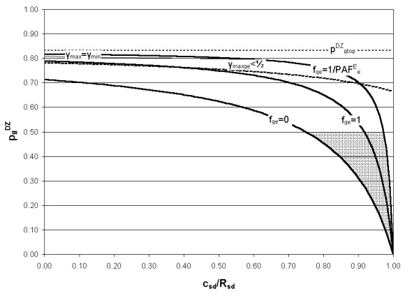
Example model solution space with RMD < 1+RSD and Uge ≥ 0. Input parameters: λMZ = 3.4, λDZ = 3, λsib = 2, ε = 0.2, PAFEe = 0.5, cMD = 1, rt = 0.1. Hence RMD = 1.2, RSD = 0.5.
Figure 3.
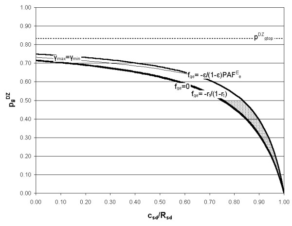
Example model solution space with RMD < 1+RSD and Uge ≤ 0. Input parameters as for Figure 2.
Figure 4.
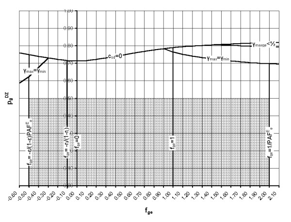
Example full model solution space with RMD < 1+RSD. Input parameters as for Figure 2, with the solution space transformed so that fge is on the horizontal axis.
For lower values of RMD, the curves defining the solution space are shifted downwards [see Additional files 2 to 9], so that the line fge = 0 (corresponding to no gene-environment interaction) lies entirely below the line pDZg = 1/2 (corresponding to an additive genetic model). The classical twin study solution does not exist, but many other combinations of genetic and gene-environment interaction models may fit the data.
When cMD > 1, lines of constant fge no longer decrease monotonically to zero, and are also shifted upwards, so that solutions with strong G-E interactions are no longer possible [see Additional files 10 to 12].
Example applications using twin, sibling and environmental data
Input values
Consider example applications of the model for male lung cancer, female breast cancer and schizophrenia. The model input variables used are shown in Table 7.
Table 7.
Input variables
| Condition | λMZ | λDZ | λsib | ε | PAFEe | rt |
| Breast cancer | 4.09 | 2.51 | 2.01 | 0.62 | 0.15 | 0.036 |
| Lung cancer | 6.27 | 6.14 | 3.16 | 0.15 | 0.86 | 0.017 |
| Schizophrenia | 52.1 | 14.2 | 8.6 | 0.62 | 0.15 | 0.01 |
| 0.15 | 0.86 | |||||
The recurrence risks, λ, and total risks, rt, for breast and lung cancer are those calculated by Risch [30], based on Scandinavian twin data reported by Lichtenstein et al. [31] (involving more than 44,000 twin pairs) and Swedish familial data reported by Doug and Hemminki [32] (involving more than 2 million families). The proportion of the population exposed, ε, and population attributable fraction, PAFEe, for breast cancer are taken from those reported by Rockhill et al. [33] for a US population. Although strictly speaking these values may not be appropriate for a Scandinavian population, and include a component due to family history that may be (at least partly) genetic, they give a low Ve, consistent with the known environmental risk factors for breast cancer, and results are not sensitive to these input values (because Ve is so small). For lung cancer, it is assumed that 15% of the Scandinavian population smokes and that 86% of lung cancer cases could be avoided if they did not (giving a risk of lung cancer in smokers of 10%).
The recurrence risks λ, and total risk, rt, for schizophrenia are those used by Risch [16], based on European data summarized by McGue et al. [34]. More recent twin studies for schizophrenia have given variable results and this example should be treated as illustrative only. Further, environmental exposures and population attributable fractions are unknown for schizophrenia. Two exploratory sets of results are therefore reported, using data consistent with a low environmental variance (based on the values used for breast cancer), and high environmental variance (based on the values used for smoking and lung cancer).
Detailed results for the three diseases are shown in [Additional file 13, 14, 15, 16, 17, 18, 19, 20, 21, 22, 23, 24, 25, 26, 27, 28, 29, 30, 31, 32, 33]. The key findings are outlined below.
Breast cancer results
For breast cancer, the PAFEe associated with known environmental factors is low. The value of the model is therefore less in calculating the utility of targeted environmental interventions than in exploring the solution space for a complex disease with RMD close to 2.
Although strictly speaking the classical twin study solution (with an additive genetic model, pDZg = 1/2, and an additive G-E model, fge = 0) does not exist as a solution, it might lie within the margin of error of the data. However, an infinite number of other models also could also fit the data. The classical twin model result always overestimates the genetic component of the variance, which reduces as the gene-environment interaction factor fge increases, and also as pDZg decreases (i.e. as epistatic terms begin to dominate the genetic model). These alternative models imply that shared environmental factors may partially explain familial aggregation of breast cancer. This contrasts with the classical twin method result (see earlier), which for RMD = 2 leads to the inevitable conclusion that shared sibling risk must be due solely to shared genes [35].
In theory, a model with pDZg = 0 (where shared sibling risk is due entirely to shared environmental factors) could fit the data. However, for breast cancer the existence of known mutations that significantly increase risk (particularly mutations in the BRCA1 and BRCA2 genes, which are relatively common) rules out this solution. Although it is not possible to subtract out the effect of these mutations from the model, it is possible to show that they could be sufficient to explain the twin data if a G-E interaction also exists. For example, one possible solution consistent with the data could involve one or more dominant genes (pDZg = 1/2), a strong G-E interaction (fge = 1/PAFE e), but a largely environmental explanation for shared sibling risk (say cSD/RSD = 0.9). This solution implies that the genetic component of the variance is less than a fifth of the classical twin study result, which could be low enough to be explained by mutations in the BRCA1 and BRCA2 genes alone [35]. If this model were correct it would have important implications for women with such mutations, but would not contribute significantly to reducing the incidence of breast cancer in the population as a whole, because the affected proportion of the population γ would be rather small. Other solutions, involving different genetic models with lower pDZg, and/or less gene-environment interaction, are also possible.
The line γmax = γmin does not occur within the solution space for breast cancer; however, in some circumstances the lines γmax and γmin may be rather close together. This suggests that, although as expected there is always a trade-off between selecting a small proportion (γmin) of the population with a high Positive Predictive Value (PPV), or a larger proportion of the population (γmax) with a higher Population Impact (PI) [19], some possible solutions could exist for breast cancer where the PPV and PI are both relatively high. Further, γmax is often less than 1/2, so that, in these regions of the possible solution space, maximum utility might be obtained by targeting less than 50% of the population. However, known environmental factors for breast cancer are often not amenable to intervention and other possible solutions, with low, zero or negative utility, also exist.
Lung cancer results
For lung cancer, all the possible solutions imply that shared sibling risk is largely due to shared environmental factors (smoking) because solutions occur only when cSD/RSD is close to 1. Unlike for breast cancer, the line γmax = γmin lies outside the solution space, even for negative fge, as does the area of solutions with γmaxge < 1/2. However, the classical twin study solution, with fge = 0 and pDZg = 1/2, clearly lies within the solution space.
Although the classical twin model again provides an upper limit to the genetic component of the variance, even the classical result indicates that the risk of lung cancer is dominated by smoking in this population and the variance has at most a small genetic component.
Unlike the breast cancer example, γmax and γmin are always far apart, suggesting a strong trade off between high Postive Predictive Value (Rge) for a genotypic test and a high Population Impact (PI) for a targeted intervention. This means that a genotypic test that predicts which smokers will get lung cancer cannot exist. To predict all cases of lung cancer in smokers (i.e. to obtain PI = 1), 95% or more of the population would have to be in the high genotypic risk group, and the predictive value of such a test would be very low.
Because the genetic component of the variance is so small, it follows that the utility of genetic 'prediction and prevention' (measured by Uge) is also small (from Equation (28)). Utility is maximum when γ = 1/2, but even then values are low. The maximum utility of genotyping occurs when about 60% of cases could be prevented by targeting the 50% of smokers at high genotypic risk. However, other possible solutions have zero or negative utility.
Schizophrenia results
For schizophrenia, the classical twin study solution (with fge = 0 and pDZg = 1/2 and cMD = 1) cannot not fit the data. If the 'equal environments' assumption holds, neither a single dominant gene (pDZg = 1/2), nor additive polygenic model (also with pDZg = 1/2), nor single recessive gene (pDZg = 1/4) can explain the twin and family data, consistent with Risch's 1990 findings [16]. This may suggest that the genetic model for schizophrenia is likely to be dominated by epistatic terms. However, if gene-environment interactions are important, it is also possible that a recessive gene, combined with at least multiplicative G-E interaction (pDZg = 1/4 and fge = 1 or higher), could explain the data.
The possible solution spaces include purely genetic explanations for shared sibling risk (at cSD/RSD = 0), or purely environmental ones (at cSD/RSD = 1, applicable if pDZg = 0).
Assuming a small environmental component to the variance, there is no region of the solution space for which γmaxge < 1/2, suggesting that the utility of targeted environmental interventions under these assumptions is likely to be low. However, if the environmental component of the variance is assumed to be much larger, the available solution space changes dramatically, because the line γmax = γmin now constrains the solution space to a much smaller area, which excludes solutions with no G-E interaction (fge = 0). Special solutions may exist along the line γmax = γmin, as shown in Table 5. Because the environmental factors contributing to schizophrenia are unknown, it is impossible to draw any conclusions about the potential benefits of targeting environmental interventions at those at high genotypic risk.
Because prenatal development is thought to be important in schizophrenia, it is plausible that monozygotic twins are more likely to share environmental risk factors than dizygotic twins are. Breaking the 'equal environments' assumption changes the shape of the solution space significantly, and, assuming a small environmental component to the variance, only limited G-E interactions are now possible (the multiplicative G-E model, fge = 1, lies largely outside the solution space). The utility of targeting environmental interventions by genotype is then likely to be low. However, in these circumstances it is possible that an additive genetic model (pDZg = 1/2) with some G-E interaction, or a recessive gene (pDZg = 1/4) with no G-E interaction, could explain the data.
Discussion
If Fisher's polygenic model [26] is abandoned, along with the usual twin study assumption that there are no gene-environment interactions, the four-category model developed by Khoury and others can be combined with twin, family and environmental data to implement a 'top down' approach to assessing the utility of targeting environmental/lifestyle interventions by genotype. Scoping studies, valid when RSD ≠ 1, provide a first step to modelling the health of populations [23].
Abandoning Fisher's assumption that the polygenic model is necessarily dominated by an additive term can be justified by the growing evidence that phenotypic effects can result from the synergistic action of alleles in many genes [36]. For example, Bardet-Biedl Syndrome, historically assumed to be a recessive trait, has been shown to involve three interacting mutations at two loci in some patients (implying that pDZg = 1/8) and, more recently, an additional locus has been identified that can also interact to change disease severity and symptoms [37]. Both positive and negative gene-environment interactions have also been observed in human diseases, although there are difficulties in confirming their statistical validity [38,39].
The model also allows the impact of the much criticised 'equal environments' assumption to be explored.
A number of conclusions can be drawn about the merits of the classical twin study and the utility of genetic 'prediction and prevention'.
Firstly, the model confirms that the classical twin study solution is not always valid and gives at best an upper limit to the genetic component of the variance of a trait. The importance of the 'equal environments' assumption and of gene-environment interactions have previously been recognised [17,18]; however, less attention has been paid to the potential role of gene-gene interactions (epistasis). For larger values of RMD (greater than 1+RSD), observed for conditions such as schizophrenia, the model generalizes Risch's findings [16] to show that the three assumptions of the classical twin model cannot all be satisfied simultaneously. For intermediate RMD values, observed for conditions such as breast cancer (for which RMD is approximately 2), the model illustrates that the conclusion drawn from classical twin studies, that familial aggregation is due entirely to shared genetic factors, may be erroneous. This raises the possibility – previously rejected on the basis of twin study results [35] – that genetic variants are important in determining risk only for the relatively rare familial forms of cancer. If so, genetic models of familial aggregation (for example [40]) may be incorrect and the hunt for additional susceptibility genes could be largely fruitless. Existing published findings might then reflect prevailing bias, rather than true associations [14].
Secondly, the model confirms that the potential for reducing the incidence of common diseases using environmental/lifestyle interventions targeted by genotype may be limited [7] by:
(i) the low importance of genetic differences in determining the risk of some conditions (for example, lung cancer);
(ii) the complexity of gene-gene and gene-environment interactions and/or lack of knowledge of environmental factors (for example, schizophrenia).
Targeting environmental/lifestyle interventions at those at 'high genotypic risk' can be of high utility only in specific circumstances. The utility of targeting environmental interactions by genotype (compared to randomly selecting the same number of people from the population) is zero if there is no gene-environment interaction. Utility can also be negative in the presence of a negative interaction (i.e. if the people at high genotypic risk have less to gain by the intervention than people at low genotypic risk). The finding that utility increases with gene-environment interaction is consistent with Khoury and Wagener [19] but the relationship is considerably clarified by the adoption here of different measures of the population attributable fraction associated with a targeted intervention (PAFEge) and of utility (Uge). Further, by formally introducing constraints on the model (for example, that risks are positive and do not exceed 100%), it is possible to demonstrate that both the gene-environment interaction factor and utility have maximum values, which cannot be exceeded for a given data set.
The lung cancer example is apparently trivial but also of critical importance. The RMD value for lung cancer is close to 1, and neither the Scandinavian data used here [31], nor earlier US studies [41], have identified a significant heritable component. It follows from Equation (27) that if the genetic component of the variance, Vg, is zero, Vge (the G-E component of the variance) is also zero and using genotyping to target an intervention such as smoking cessation is therefore of zero utility (no better than randomly selecting the same number of individuals). This approximate conclusion is confirmed by the results presented for lung cancer, which show extremely low utility. The detailed calculations may at first sight seem unnecessary, particularly because smoking causes multiple diseases and targeting smoking cessation on the basis of lung cancer risk alone is therefore ill-advised. However, the idea that a genetic test will one day predict which smokers get lung cancer has been widely promoted in the literature and has driven much research aimed at identifying the supposed 'genes for lung cancer' [42]. The results presented here strongly suggest that there will never be a genetic or genotypic test that predicts which smokers will get lung cancer, because the genetic component of the variance is not high enough.
Finally, the model illustrates the argument of Terwilliger and Weiss [11] that the potential for population biobanks to quantify risks for complex disease is limited by a 'multiple testing' problem caused by the large number of genetic and gene-environment interaction models that could fit existing data. Each point in each solution space described above represents a different combination of a genetic risk model (defined by pDZg) and a G-E interaction model (defined by fge). Further, any given value of pDZg may be obtained by an infinite number of different combinations of different alleles acting through multiple biological pathways. Because the number of hypotheses that could be tested is essentially infinite, sample sizes necessary to quantify the risks (Roo, Rgo, Roe and Rge) could "plausibly be larger than the number of people that have ever lived" [11].
The model has several limitations. Measurements of shared sibling risk (λsib) are needed from the same population as twin data, and the scoping studies are only valid for λDZ > λsib, implying that environmental risks are more strongly correlated in dizygotic twins than other siblings. Some data exist to support this assumption for smoking [43] but for other exposures its validity is usually unknown. However, the model does not reduce to the classical twin study solution if this condition is not met: instead, data from more relatives are needed. In principle the model could, and should, be expanded to include data from more relatives, other data (such as migration study data), more risk categories and error terms. However, the number of unknown parameters will then increase, unless more data are available to quantify exposures (which change from generation to generation) and to estimate the extent to which environments are correlated between different types of relative.
Treating exposure and environmental variance (or population attributable fraction) as input data is also problematic when the effects of environmental factors on risk are often unknown. Further, the simple nature of the model (with one environmental axis) cannot adequately represent the complexity of environmental (including socio-economic) causes of disease. However, if targeting environmental interventions by genotype is to be considered, this implies that at least something is known (or expected to be learned) about environmental factors, such as particular exposures, that are amenable to intervention.
The assumption of no gene-environment correlation will often hold (for example it is rather implausible that the same genes strongly influence both lung cancer risk and nicotine addiction), but is not necessarily always true. Adult lactose intolerance is an example of a condition with a strong gene-environment interaction where targeted intervention to avoid drinking milk may be of high utility. However, the model is invalid for lactose intolerance unless exposures are applied equally to the population studied because, in general, people who are lactose intolerant may be less likely to drink milk (a gene-environment correlation) owing to the unpleasant symptoms.
A more fundamental problem is caused by the assumptions that: (i) the risks Roo, Rgo, Roe and Rge are inherent properties of a given trait within a given population (with a given γ and ε) and that there are therefore no confounders; and (ii) risks are randomly distributed within these categories.
These assumptions, although often made, are implausible in many situations. The assumption of no confounders means that the model can only represent a subset of the potential models of gene-gene and gene-environment interaction described by more complex models (for example [17]). It is unlikely to be met if multiple genetic factors interact with multiple environmental ones [44]. Although this may well render the results presented here invalid, such complexity is likely to reduce the utility of targeting by genotype, rather than enhance it. Hence, situations where the 'no confounders' assumption at least approximately holds are those most likely to be of relevance to public health.
The second assumption neglects the fact that for most exposures there is a gradient in risk, with higher exposure meaning higher risk, and that the same may also be true of genetic factors. This means that increasing the number of categories in the model will increase Ve (see [45]) and perhaps Vg. Further, these subcategories may be differently correlated between relatives (for example, the twin of a heavy smoker may be more likely to be a heavy smoker than a light one). If so, a relative of a proband may not be representative of their allocated risk category in the four-category model and Equation (22) then becomes invalid.
More broadly, these assumptions make the model, like the classical twin model, essentially deterministic: it assumes that all the factors contributing to correlations in risk between relatives are perfectly known and are either environmental or genetic. Retention of these assumptions here may be problematic and could limit the applicability of the results. Nevertheless, all the other questionable assumptions of the classical twin model have been simultaneously removed.
Conclusion
The model shows that the potential for reducing the incidence of common diseases using environmental interventions targeted by genotype may be limited, except in special cases. The model also confirms that the importance of an individual's genotype in determining their risk of complex diseases tends to be exaggerated by the classical twin studies method, owing to the 'equal environments' assumption and the assumption of no gene-environment interaction. In addition, if phenotypes are genetically robust, because of epistasis, a largely environmental explanation for shared sibling risk is plausible, even if the classical heritability is high. The model therefore highlights the possibility – previously rejected on the basis of twin study results – that inherited genetic variants are important in determining risk only for the relatively rare familial forms of diseases such as breast cancer. If so, genetic models of familial aggregation may be incorrect and the hunt for additional susceptibility genes could be largely fruitless.
Competing interests
The author(s) declare that they have no competing interests.
Appendix A: formal derivation of equation (31)
Equation (23) may be derived more formally by extending the matrix method of Li and Sacks [46].
Define the probability that an affected proband is in genotypic risk category z and environmental risk category w as Pzw and assume that risks are randomly distributed within categories. Using the definitions of the four category model given in Table 1, a vector P may be defined:
A risk vector R may also be defined:
Now define Gxy as the conditional probability P(relative is in genotypic risk category y|proband is in genotypic risk category x). Similarly, define Exy as the conditional probability P(relative is in environmental risk category y|proband is in environmental risk category x). Using the definitions of prelg and prele given in Section 2.5, matrices G and E may be written such that:
Finally, define Xab-cd as the conditional probability P(relative is in risk category cd|proband is in risk category ab), where the risk categories are as defined in Table 1 (for example risk categorgy 'ge' implies high-genotypic and high-environmental risk). Provided prelg and prele are independent (there are no gene-environment correlations), the gene-environment interaction matrix Mrelge may be written as:
Then the risk in a relative of the proband is given by:
After some algebra, this yields equation (23).
Appendix B: calculating recurrence risks for twins
The sibling recurrence risk λsib is often available directly from familial studies. For twins the recurrence risks, if not reported, may be calculated from the case-wise concordance (Cc):
λMZ = CcMZ /rt (B1)
λDZ = CcDZ /rt (B2)
where, if there is complete ascertainment of all affected twins in a population,
Cc = 2C/(2C + D) (B3)
and C is the number of concordant and D the number of discordant pairs [25].
Supplementary Material
Gene-gene and gene-environment interaction model. Contains the Visual Basic macro (Twincal), input and output datasheets and charts used to calculate the solutions described in the text. The program is run by entering parameters in the 'Inputs' sheet and clicking on the 'Run' button. Note that for the final chart ('fe') the number of categories on the horizontal axis changes depending on the environmental input parameters ε and PAFEe. If these parameters are changed it is therefore necessary to delete the lower part of the output sheet prior to running the model and, after the run, to redraw the chart using the source data option from the chart. All other charts are drawn automatically. The line γmax = γmin is calculated exactly for the chart 'fe' but is approximated in the charts 'pgdz' and 'pgdzneg' using Newton's method and an initial guess for fge (f0) and step (fet). For some input parameters it may be necessary to change these values by editing the Visual Basic code (Twincal) to obtain a valid solution.
Supplementary Figure 1: Example model solution space with RMD = 1.7 and Uge ≥ 0. Model solution space with Uge ≥ 0 for the same input parameters as Figure 2, apart from λMZ = 4.4.
Supplementary Figure 2: Example model solution space with RMD = 1.8 and Uge ≥ 0. Model solution space with Uge ≥ 0 for the same input parameters as Figure 2, apart from λMZ = 4.6.
Supplementary Figure 3: Example model solution space with RMD = 1.95 and Uge ≥ 0. Model solution space with Uge ≥ 0 for the same input parameters as Figure 2, apart from λMZ = 4.9.
Supplementary Figure 4: Example model solution space with RMD = 2.1 and Uge ≥ 0. Model solution space with Uge ≥ 0 for the same input parameters as Figure 2, apart from λMZ = 5.2.
Supplementary Figure 5: Example full solution space with RMD = 1.7. Full model solution space for the same input parameters as Figure 5, transformed so that fge is on the horizontal axis.
Supplementary Figure 6: Example full solution space with RMD = 1.8. Full model solution space for the same input parameters as Figure 6, transformed so that fge is on the horizontal axis.
Supplementary Figure 7: Example full solution space with RMD = 1.95. Full model solution space for the same input parameters as Figure 7, transformed so that fge is on the horizontal axis.
Supplementary Figure 8: Example full solution space with RMD = 2.1. Full model solution space for the same input parameters as Figure 8, transformed so that fge is on the horizontal axis.
Supplementary Figure 9: Example model solution with cMD > 1 and Uge ≥ 0. Input parameters: λMZ = 5.2, λDZ = 3, λsib = 2, ε = 0.2, PAFEe = 0.5, cMD = 2, rt = 0.1.
Supplementary Figure 10: Example model solution with cMD > 1 and Uge ≥ 0. Input parameters as for Figure 13.
Supplementary Figure 11: Example full solution space with cMD > 1. Full model solution space for the same parameters as Figure 13, transformed so that fge is on the horizontal axis.
Supplementary Figure 12: Breast cancer solution space with Uge ≥ 0. Input parameters are as shown in Table 5, with cMD = 1. The solution space is shown (shaded) for positive fge, assuming the 'equal environments' assumption holds (cMD = 1). The darker shaded area shows the part of the solution space for which γmaxge < 1/2. Utility Uge is at its maximum when γ = 1/2 except within this darker shaded area.
Supplementary Figure 13: Breast cancer variances with fge = 0. Input parameters as for Figure 16. Additive model of G-E interaction (fge = 0). Variance components are genetic (Vg) or environmental (Ve).
Supplementary Figure 14: Breast cancer variances with fge = 1. Input parameters as for Figure 16. Multiplicative G-E interaction model (fge = 1). Variance components are genetic (Vg), environmental (Ve) or due to gene-environment interaction (Vge).
Supplementary Figure 15: Breast cancer variances with fge = 1/PAFEe. Input parameters as for Figure 16. Maximum G-E interaction model (fge = 1/PAFEe). Variance components are genetic (Vg), environmental (Ve) or due to gene-environment interaction (Vge).
Supplementary Figure 16: Breast cancer γ values with fge = 0. Input parameters as for Figure 16. The proportion of the population in the 'high genotypic risk' group, γ, may take any value in the shaded area. γmin occurs when Rge = 1, i.e. when the Positive Predictive Value (PPV) of being in the 'ge' subgroup is 100%. γmax occurs when Roo = 1 for an additive G-E model and solutions with a Population Impact of 100% (PI = 1) cannot exist.
Supplementary Figure 17: Breast cancer γ values with fge = 1. Input parameters as for Figure 16. The proportion of the population in the 'high genotypic risk' group, γ, may take any value in the shaded area. A solution with a Population Impact of 100% (PI = 1) may exist if γ = γmax.
Supplementary Figure 18: Breast cancer γ values with fge = 1/PAFEe. Input parameters as for Figure 16. The proportion of the population in the 'high genotypic risk' group, γ, may take any value in the shaded area. A solution with a Population Impact of 100% (PI = 1) may exist if γ = γmax.
Supplementary Figure 19: Breast cancer solution space with Uge ≤ 0. Input parameters are as for Figure 16. The solution space is shown for negative fge (where the utility of targeting environmental interventions at the high genotypic risk group is negative, Uge ≤ 0). Solutions exist only in the shaded area where γmax ≥ γmin.
Supplementary Figure 20: Breast cancer: full solution space. Input parameters are as for Figure 16. The same solution space as Figures 16 and 23 is shown (shaded), transformed so that the G-E interaction factor is plotted on the horizontal axis. Again, each point in the shaded solution space represents a genetic model defined by pDZg and a G-E interaction model defined by fge. The area of solutions with γmaxge < 1/2 is highlighted with darker shading. The classical twin study solution lies on the vertical axis (fge = 0) at the point pDZg = 1/2, and is slightly outside the solution space.
Supplementary Figure 21: Lung cancer solution space with Uge ≥ 0. Input parameters are as shown in Table 5, with cMD = 1.
Supplementary Figure 22: Lung cancer variances with fge = 0. Input parameters as for Figure 25. Note that the horizontal axis has been expanded to show high values of cSD/RSD only.
Supplementary Figure 23: Lung cancer variances with fge = 1. Input parameters as for Figure 25. Note that the horizontal axis has been expanded to show high values of cSD/RSD only.
Supplementary Figure 24: Lung cancer variances with fge = 1/PAFEe. Input parameters as for Figure 25. Note that the horizontal axis has been expanded to show high values of cSD/RSD only.
Supplementary Figure 25: Lung cancer γ values for fge = 1. Input parameters as for Figure 25. The proportion of the population in the 'high genotypic risk' group, γ, may take any value in the shaded area.
Supplementary Figure 26: Lung cancer γ values for fge = 1/PAFEe. Input parameters as for Figure 25. The proportion of the population in the 'high genotypic risk' group, γ, may take any value in the shaded area.
Supplementary Figure 27: Lung cancer Uge values for fge = 1. Input parameters as for Figure 25. The utility parameter, Uge, may take any value in the shaded area, but is maximum when γ = 1/2.
Supplementary Figure 28: Lung cancer Uge values for fge = 1/PAFEe. Input parameters as for Figure 25. The utility parameter, Uge, may take any value in the shaded area, but is maximum when γ = 1/2.
Supplementary Figure 29: Lung cancer: full solution space. Input parameters as for Figure 25.
Supplementary Figure 30: Schizophrenia Uge ≥ 0, small environmental variance and cMD ≥ 1. Input parameters are as shown in Table 5, with ε = 0.62, PAFEe = 0.15 and cMD = 1.
Supplementary Figure 31: Schizophrenia Uge ≥ 0, small environmental variance and cMD > 1. Input parameters are as shown in Table 5, with ε = 0.62, PAFEe = 0.15 and cMD = 3.8.
Supplementary Figure 32: Schizophrenia Uge ≥ 0, large environmental variance and cMD = 1. Input parameters are as shown in Table 5, with ε = 0.15, PAFEe = 0.86 and cMD = 1.
Acknowledgments
Acknowledgements
The author is grateful to the Joseph Rowntree Charitable Trust for funding the completion of this work.
References
- Collins FS. Shattuck Lecture – medical and societal consequences of the Human Genome Project. New Engl J Med. 1999;341:28–37. doi: 10.1056/NEJM199907013410106. [DOI] [PubMed] [Google Scholar]
- Bell J. The new genetics in clinical practice. BMJ. 1998;316:618–620. doi: 10.1136/bmj.316.7131.618. [DOI] [PMC free article] [PubMed] [Google Scholar]
- Collins FS, McKusick VA. Implications of the Human Genome Project for medical science. J Am Med Assoc. 2001;285:540–544. doi: 10.1001/jama.285.5.540. [DOI] [PubMed] [Google Scholar]
- Strohman RC. The coming Kuhnian revolution in biology. Nat Biotechnol. 1997;15:194–200. doi: 10.1038/nbt0397-194. [DOI] [PubMed] [Google Scholar]
- Holtzman NA, Marteau TM. Will genetics revolutionize medicine? New Engl J Med. 2000;343:141–144. doi: 10.1056/NEJM200007133430213. [DOI] [PubMed] [Google Scholar]
- Vineis P, Schulte P, McMichael AJ. Misconceptions about the use of genetic tests in populations. Lancet. 2001;357:709–712. doi: 10.1016/S0140-6736(00)04136-2. [DOI] [PubMed] [Google Scholar]
- Baird P. The Human Genome Project, genetics and health. Community Genet. 2001;4:77–80. doi: 10.1159/000051161. [DOI] [PubMed] [Google Scholar]
- Cooper RS, Psaty BM. Genetics and medicine: distraction, incremental progress, or the dawn of a new age? Ann Intern Med. 2003;138:576–580. doi: 10.7326/0003-4819-138-7-200304010-00014. [DOI] [PubMed] [Google Scholar]
- Vineis P, Ahsan H, Parker M. Genetic screening and occupational and environmental exposures. Occup Environ Med. 2004;62:657–662. doi: 10.1136/oem.2004.019190. [DOI] [PMC free article] [PubMed] [Google Scholar]
- Khoury MJ, Yang Q, Gwinn M, Little J, Flanders WD. An epidemiologic assessment of genetic profiling for measuring susceptibility to common diseases and targeting interventions. Genet Med. 2004;6:38–47. doi: 10.1097/01.gim.0000105751.71430.79. [DOI] [PubMed] [Google Scholar]
- Terwilliger JD, Weiss KM. Confounding, ascertainment bias, and the blind quest for a genetic 'fountain of youth'. Ann Med. 2003;35:532–544. doi: 10.1080/07853890310015181. [DOI] [PubMed] [Google Scholar]
- Ioannidis JPA, Ntzani EE, Trikalinos TA, Contopoulos-Ionnidis DG. Replication validity of genetic association studies. Nat Genet. 2001;29:306–309. doi: 10.1038/ng749. [DOI] [PubMed] [Google Scholar]
- Cordell HJ, Clayton DG. Genetic association studies. Lancet. 2005;366:1121–1131. doi: 10.1016/S0140-6736(05)67424-7. [DOI] [PubMed] [Google Scholar]
- Ioannidis J. Why most published research findings are false. PloS Med. 2005;2:e124. doi: 10.1371/journal.pmed.0020124. DOI: 10.137/journal.pmed.0020124. [DOI] [PMC free article] [PubMed] [Google Scholar]
- Layzer D. Heritability analyses of IQ scores: science or numerology? Science. 1974;183:1259–1266. doi: 10.1126/science.183.4131.1259. [DOI] [PubMed] [Google Scholar]
- Risch N. Linkage strategies for genetically complex traits. I. Multilocus models. Am J Hum Genet. 1990;46:222–228. [PMC free article] [PubMed] [Google Scholar]
- Guo S-W. Gene-environment interaction and the mapping of complex traits: some statistical models and their interpretation. Hum Hered. 2000;50:286–303. doi: 10.1159/000022931. [DOI] [PubMed] [Google Scholar]
- Hopper JL. Why 'common environmental effects' are so uncommon in the literature. In: Spector TD, Sneider H, MacGregor AJ, editor. Advances in twin and sib-pair analysis. London: Greenwich Medical Media Ltd; 2000. [Google Scholar]
- Khoury MJ, Wagener DK. Epidemiological evaluation of the use of genetics to improve the predictive value of disease risk factors. Am J Hum Genet. 1995;56:835–844. [PMC free article] [PubMed] [Google Scholar]
- Lewis SJ, Brunner EJ. Methodological problems in genetic association studies of longevity – the apolipoprotein E gene as an example. Int J Epidemiol. 2004;33:962–970. doi: 10.1093/ije/dyh214. [DOI] [PubMed] [Google Scholar]
- Tryggvadottir L, Sigvaldason H, Olafsdottir GH, Jonasson JG, Jonsson T, Tulinius H, Eyfjord JE. Population-based study of changing breast cancer risk in Icelandic BRCA2 mutation carriers, 1920–2000. J Natl Cancer Inst. 2006;98:116–122. doi: 10.1093/jnci/djj012. [DOI] [PubMed] [Google Scholar]
- Humphries S, Ridker PM, Talmud PJ. Genetic testing for cardiovascular disease susceptibility: a useful clinical management tool or possible misinformation? Arterioscler Thromb Vasc Biol. 2004;24:628–636. doi: 10.1161/01.ATV.0000116216.56511.39. [DOI] [PubMed] [Google Scholar]
- Rose G. Sick individuals and sick populations. Int J Epidemiol. 1985;14:32–38. doi: 10.1093/ije/14.1.32. [DOI] [PubMed] [Google Scholar]
- Khoury MJ, Jones K, Grosse SD. Quantifying the health benefits of genetic tests: The importance of a population perspective. Genet Med. 2006;8:191–195. doi: 10.1097/01.gim.0000206278.37405.25. [DOI] [PubMed] [Google Scholar]
- MacGregor AJ. Practical approaches to account for bias and confounding in twin data. In: Spector TD, Sneider H, MacGregor AJ, editor. Advances in twin and sib-pair analysis. London: Greenwich Medical Media Ltd; 2000. [Google Scholar]
- Fisher RA. The correlation between relatives on the supposition of Mendelian inheritance. Trans R Soc Edinb. 1918;52:399–433. [Google Scholar]
- Hopper JL. Variance components for statistical genetics: applications in medical research to characteristics related to human diseases and health. Stat Methods Med Res. 1993;2:199–223. doi: 10.1177/096228029300200302. [DOI] [PubMed] [Google Scholar]
- Porteous JW. A rational treatment of Mendelian genetics. Theor Biol Med Model. 2004;1:6. doi: 10.1186/1742-4682-1-6. DOI: 10.1186/1742-4682-1-6. [DOI] [PMC free article] [PubMed] [Google Scholar]
- Azevedo RBR, Lohaus R, Srinivasan S, Dang KK, Burch CL. Sexual reproduction selects for robustness and negative epistasis in artificial gene networks. Nature. 2006;440:87–90. doi: 10.1038/nature04488. [DOI] [PubMed] [Google Scholar]
- Risch N. The genetic epidemiology of cancer: interpreting family and twin studies and their implications for molecular genetic approaches. Cancer Epidemiol Biomarkers Prev. 2001;10:733–741. [PubMed] [Google Scholar]
- Lichtenstein P, Holm NV, Verkasalo PK, Iliadou A, Kaprio J, Koskenvuo M, Pukkala E, Skytthe A, Hemminki K. Environmental and heritable factors in the causation of cancer. New Engl J Med. 2000;343:78–85. doi: 10.1056/NEJM200007133430201. [DOI] [PubMed] [Google Scholar]
- Dong C, Hemminki K. Modification of cancer risks in offspring by sibling and parental cancers from 2,112,616 nuclear families. Int J Cancer. 2001;92:144–150. doi: 10.1002/1097-0215(200102)9999:9999<::AID-IJC1147>3.0.CO;2-C. [DOI] [PubMed] [Google Scholar]
- Rockhill B, Weinberg CR, Newman B. Population attributable fraction estimation for established breast cancer risk factors: considering the issues of high prevalence and unmodifiability. Am J Epidemiol. 1998;147:826–833. doi: 10.1093/oxfordjournals.aje.a009535. [DOI] [PubMed] [Google Scholar]
- McGue M, Gottesman II, Rao DC. The transmission of schizophrenia under a multifactorial threshold model. Am J Hum Genet. 1983;35:1161–1178. [PMC free article] [PubMed] [Google Scholar]
- Easton DF. How many more breast cancer predisposition genes are there? Breast Cancer Res. 1999;1:14–17. doi: 10.1186/bcr6. [DOI] [PMC free article] [PubMed] [Google Scholar]
- Badano JL, Katsanis N. Beyond Mendel: an evolving view of human genetic disease transmission. Nat Rev Genet. 2002;3:779–789. doi: 10.1038/nrg910. [DOI] [PubMed] [Google Scholar]
- Badano JL, Leitch CC, Ansley SJ, May-Simera H, Lawson S, Lewis RA, Beales PL, Dietz HC, Fisher S, Katsanis N. Dissection of epistasis in oligogenic Bardet-Biedl syndrome. Nature. 2006;439:326–330. doi: 10.1038/nature04370. [DOI] [PubMed] [Google Scholar]
- Taioli E, Zocchetti C, Garte S. Models of interaction between metabolic genes and environmental exposure in cancer susceptibility. Environ Health Perspect. 1998;106:67–70. doi: 10.1289/ehp.9810667. [DOI] [PMC free article] [PubMed] [Google Scholar]
- Hunter DJ. Gene-environment interactions in human diseases. Nat Rev Genet. 2005;6:287–298. doi: 10.1038/nrg1578. [DOI] [PubMed] [Google Scholar]
- Antoniou AC, Pharoah PDP, McMullan G, Day NE, Stratton MR, Peto J, Ponder BJ, Easton DF. A comprehensive model for familial breast cancer incorporating BRCA1, BRCA2 and other genes. Br J Cancer. 2002;86:76–83. doi: 10.1038/sj.bjc.6600008. [DOI] [PMC free article] [PubMed] [Google Scholar]
- Braun MM, Caporaso NE, Page WF, Hoover RN. A cohort study of twins and cancer. Cancer Epidemiol Biomarkers Prev. 1995;4:469–473. [PubMed] [Google Scholar]
- Hall W, Madden P, Lynskey M. The genetics of tobacco use: methods, findings and policy implications. Tob Control. 2002;11:119–124. doi: 10.1136/tc.11.2.119. [DOI] [PMC free article] [PubMed] [Google Scholar]
- Vink JM, Willemsen G, Boomsma DI. The association of current smoking behavior with the smoking behavior of parents, siblings, friends and spouses. Addiction. 2003;98:923–931. doi: 10.1046/j.1360-0443.2003.00405.x. [DOI] [PubMed] [Google Scholar]
- Taioli E, Garte S. Covariates and confounding in epidemiologic studies using metabolic gene polymorphisms. Int J Cancer. 2002;100:97–100. doi: 10.1002/ijc.10448. [DOI] [PubMed] [Google Scholar]
- Guo S. The behaviors of some heritability estimators in the complete absence of genetic factors. Hum Hered. 1999;49:215–228. doi: 10.1159/000022878. [DOI] [PubMed] [Google Scholar]
- Li CC, Sacks L. The derivation of joint distribution and correlation between relatives by the use of stochastic matrices. Biometrics. 1954;10:347–360. doi: 10.2307/3001590. [DOI] [Google Scholar]
Associated Data
This section collects any data citations, data availability statements, or supplementary materials included in this article.
Supplementary Materials
Gene-gene and gene-environment interaction model. Contains the Visual Basic macro (Twincal), input and output datasheets and charts used to calculate the solutions described in the text. The program is run by entering parameters in the 'Inputs' sheet and clicking on the 'Run' button. Note that for the final chart ('fe') the number of categories on the horizontal axis changes depending on the environmental input parameters ε and PAFEe. If these parameters are changed it is therefore necessary to delete the lower part of the output sheet prior to running the model and, after the run, to redraw the chart using the source data option from the chart. All other charts are drawn automatically. The line γmax = γmin is calculated exactly for the chart 'fe' but is approximated in the charts 'pgdz' and 'pgdzneg' using Newton's method and an initial guess for fge (f0) and step (fet). For some input parameters it may be necessary to change these values by editing the Visual Basic code (Twincal) to obtain a valid solution.
Supplementary Figure 1: Example model solution space with RMD = 1.7 and Uge ≥ 0. Model solution space with Uge ≥ 0 for the same input parameters as Figure 2, apart from λMZ = 4.4.
Supplementary Figure 2: Example model solution space with RMD = 1.8 and Uge ≥ 0. Model solution space with Uge ≥ 0 for the same input parameters as Figure 2, apart from λMZ = 4.6.
Supplementary Figure 3: Example model solution space with RMD = 1.95 and Uge ≥ 0. Model solution space with Uge ≥ 0 for the same input parameters as Figure 2, apart from λMZ = 4.9.
Supplementary Figure 4: Example model solution space with RMD = 2.1 and Uge ≥ 0. Model solution space with Uge ≥ 0 for the same input parameters as Figure 2, apart from λMZ = 5.2.
Supplementary Figure 5: Example full solution space with RMD = 1.7. Full model solution space for the same input parameters as Figure 5, transformed so that fge is on the horizontal axis.
Supplementary Figure 6: Example full solution space with RMD = 1.8. Full model solution space for the same input parameters as Figure 6, transformed so that fge is on the horizontal axis.
Supplementary Figure 7: Example full solution space with RMD = 1.95. Full model solution space for the same input parameters as Figure 7, transformed so that fge is on the horizontal axis.
Supplementary Figure 8: Example full solution space with RMD = 2.1. Full model solution space for the same input parameters as Figure 8, transformed so that fge is on the horizontal axis.
Supplementary Figure 9: Example model solution with cMD > 1 and Uge ≥ 0. Input parameters: λMZ = 5.2, λDZ = 3, λsib = 2, ε = 0.2, PAFEe = 0.5, cMD = 2, rt = 0.1.
Supplementary Figure 10: Example model solution with cMD > 1 and Uge ≥ 0. Input parameters as for Figure 13.
Supplementary Figure 11: Example full solution space with cMD > 1. Full model solution space for the same parameters as Figure 13, transformed so that fge is on the horizontal axis.
Supplementary Figure 12: Breast cancer solution space with Uge ≥ 0. Input parameters are as shown in Table 5, with cMD = 1. The solution space is shown (shaded) for positive fge, assuming the 'equal environments' assumption holds (cMD = 1). The darker shaded area shows the part of the solution space for which γmaxge < 1/2. Utility Uge is at its maximum when γ = 1/2 except within this darker shaded area.
Supplementary Figure 13: Breast cancer variances with fge = 0. Input parameters as for Figure 16. Additive model of G-E interaction (fge = 0). Variance components are genetic (Vg) or environmental (Ve).
Supplementary Figure 14: Breast cancer variances with fge = 1. Input parameters as for Figure 16. Multiplicative G-E interaction model (fge = 1). Variance components are genetic (Vg), environmental (Ve) or due to gene-environment interaction (Vge).
Supplementary Figure 15: Breast cancer variances with fge = 1/PAFEe. Input parameters as for Figure 16. Maximum G-E interaction model (fge = 1/PAFEe). Variance components are genetic (Vg), environmental (Ve) or due to gene-environment interaction (Vge).
Supplementary Figure 16: Breast cancer γ values with fge = 0. Input parameters as for Figure 16. The proportion of the population in the 'high genotypic risk' group, γ, may take any value in the shaded area. γmin occurs when Rge = 1, i.e. when the Positive Predictive Value (PPV) of being in the 'ge' subgroup is 100%. γmax occurs when Roo = 1 for an additive G-E model and solutions with a Population Impact of 100% (PI = 1) cannot exist.
Supplementary Figure 17: Breast cancer γ values with fge = 1. Input parameters as for Figure 16. The proportion of the population in the 'high genotypic risk' group, γ, may take any value in the shaded area. A solution with a Population Impact of 100% (PI = 1) may exist if γ = γmax.
Supplementary Figure 18: Breast cancer γ values with fge = 1/PAFEe. Input parameters as for Figure 16. The proportion of the population in the 'high genotypic risk' group, γ, may take any value in the shaded area. A solution with a Population Impact of 100% (PI = 1) may exist if γ = γmax.
Supplementary Figure 19: Breast cancer solution space with Uge ≤ 0. Input parameters are as for Figure 16. The solution space is shown for negative fge (where the utility of targeting environmental interventions at the high genotypic risk group is negative, Uge ≤ 0). Solutions exist only in the shaded area where γmax ≥ γmin.
Supplementary Figure 20: Breast cancer: full solution space. Input parameters are as for Figure 16. The same solution space as Figures 16 and 23 is shown (shaded), transformed so that the G-E interaction factor is plotted on the horizontal axis. Again, each point in the shaded solution space represents a genetic model defined by pDZg and a G-E interaction model defined by fge. The area of solutions with γmaxge < 1/2 is highlighted with darker shading. The classical twin study solution lies on the vertical axis (fge = 0) at the point pDZg = 1/2, and is slightly outside the solution space.
Supplementary Figure 21: Lung cancer solution space with Uge ≥ 0. Input parameters are as shown in Table 5, with cMD = 1.
Supplementary Figure 22: Lung cancer variances with fge = 0. Input parameters as for Figure 25. Note that the horizontal axis has been expanded to show high values of cSD/RSD only.
Supplementary Figure 23: Lung cancer variances with fge = 1. Input parameters as for Figure 25. Note that the horizontal axis has been expanded to show high values of cSD/RSD only.
Supplementary Figure 24: Lung cancer variances with fge = 1/PAFEe. Input parameters as for Figure 25. Note that the horizontal axis has been expanded to show high values of cSD/RSD only.
Supplementary Figure 25: Lung cancer γ values for fge = 1. Input parameters as for Figure 25. The proportion of the population in the 'high genotypic risk' group, γ, may take any value in the shaded area.
Supplementary Figure 26: Lung cancer γ values for fge = 1/PAFEe. Input parameters as for Figure 25. The proportion of the population in the 'high genotypic risk' group, γ, may take any value in the shaded area.
Supplementary Figure 27: Lung cancer Uge values for fge = 1. Input parameters as for Figure 25. The utility parameter, Uge, may take any value in the shaded area, but is maximum when γ = 1/2.
Supplementary Figure 28: Lung cancer Uge values for fge = 1/PAFEe. Input parameters as for Figure 25. The utility parameter, Uge, may take any value in the shaded area, but is maximum when γ = 1/2.
Supplementary Figure 29: Lung cancer: full solution space. Input parameters as for Figure 25.
Supplementary Figure 30: Schizophrenia Uge ≥ 0, small environmental variance and cMD ≥ 1. Input parameters are as shown in Table 5, with ε = 0.62, PAFEe = 0.15 and cMD = 1.
Supplementary Figure 31: Schizophrenia Uge ≥ 0, small environmental variance and cMD > 1. Input parameters are as shown in Table 5, with ε = 0.62, PAFEe = 0.15 and cMD = 3.8.
Supplementary Figure 32: Schizophrenia Uge ≥ 0, large environmental variance and cMD = 1. Input parameters are as shown in Table 5, with ε = 0.15, PAFEe = 0.86 and cMD = 1.