The Gaussian Network Model: Precise Prediction of Residue Fluctuations and Application to Binding Problems

Abstract

The single-parameter Γ matrix of force constants proposed by the Gaussian Network Model (GNM) is iteratively modified to yield native state fluctuations that agree exactly with experimentally observed values. The resulting optimized Γ matrix contains residue-specific force constants that may be used for an accurate analysis of ligand binding to single or multiple sites on proteins. Bovine Pancreatic Trypsin Inhibitor (BPTI) is used as an example. The calculated off-diagonal elements of the Γ matrix, i.e., the optimized spring constants, obey a Lorentzian distribution. The mean value of the spring constants is ∼−0.1, a value much weaker than −1 of the GNM. Few of the spring constants are positive, indicating repulsion between residues. Residue pairs with large number of neighbors have spring constants around the mean, −0.1. Large negative spring constants are between highly correlated pairs of residues. The fluctuations of the distance between anticorrelated pairs of residues are subject to smaller spring constants. The importance of the number of neighbors of residue pairs in determining the elements of the Γ matrix is pointed out. Allosteric effects of binding on a single or multiple residues of BPTI are illustrated and discussed. Comparison of the predictions of the present model with those of the standard GNM shows that the two models agree at lower modes, i.e., those relating to global motions, but they disagree at higher modes. In the higher modes, the present model points to the important contributions from specific residues whereas the standard GNM fails to do so.

INTRODUCTION

Residues of a protein in the native state exhibit large-scale fluctuations about their equilibrium positions. The extent of the fluctuations of a given residue depends predominantly on the number of its closest spatial neighbors. The mean-square fluctuation of a residue is, in general, smaller than that of another residue with a smaller number of neighbors. This observation forms the basis of the Gaussian network model (GNM) of proteins (1), which predicts the residue fluctuations in native proteins, in simple analogy with fluctuations of junction positions in Gaussian elastomeric networks (2). The fact that the size of the fluctuation domain of a junction in a Gaussian network varies inversely with the number of other junctions that share this domain is now well established (3), and serves as a plausible analogy for the protein fluctuations. The second simplifying assumption of the GNM was based on an earlier postulate (4) that because of the central limit theorem, the large-scale fluctuations of residues could be characterized by a single-parameter Gaussian energy function. According to this approximation, all the C^α-C^α interactions as well as the strength of the covalent bonds are assumed identical. The simplification introduced by adopting a single-parameter representation of fluctuations by Tirion (4) and Bahar et al. (1) is notable. Several articles (5–10) following the original GNM article showed that a simple harmonic potential with a single interaction-parameter indeed captures the basic physics underlying the equilibrium fluctuations in proteins. However, a closer and more careful examination of the articles comparing experiment with GNM predictions (7,9,10) shows that if the single-parameter potential is replaced by a potential that somehow reflects the environment of a given residue in more detail, the agreement between theory and experiment will be further improved. The specific aim of this article is to introduce a simple method for calculating the environment-dependent interaction parameters for a protein when its B-factors are given. We do this by iteratively modifying the residue-residue interaction parameters, until the recalculated Γ matrix of the system yields the experimentally observed mean-square residue fluctuations. The starting Γ matrix is that of the GNM. The parameters of the optimized Γ matrix then give the strength of the residue-specific pairwise interactions, which are corrections to the single-parameter GNM.

Micheletti et al. (8) used a self-consistent Gaussian model to study the equilibrium behavior of proteins in which the pairwise interactions are not equivalent, but are amino-acid specific. Starting with a Hamiltonian similar to that of the GNM, they introduced an iterative self-consistent approach for calculating the equilibrium probabilities of the contacting pairs of residues. Their work clearly shows the importance of differentiating pairwise interactions in a protein in the native state and gives the method of calculation. The approach of this article is similar to their iterative method.

In the next section, we critically review the GNM and point out to what may be missing in the model. In Theory, below, we describe the computational scheme for reevaluating the spring constants to match experimental data. As an application, we determine the spring constants for the protein Bovine Pancreatic Trypsin Inhibitor (BPTI; PDB code No. 5PTI) and present an extensive discussion of the residue-specific spring constants that lead to precise description of the observed B-factors. The present model gives a consistent theoretical description of the B-factors. A precise and consistent description of the fluctuations in proteins is of great consequence for a quantitative understanding of protein function, ligand binding, and protein-protein interactions. We discuss different possible applications of the model using the optimized values of the spring constants.

THEORY

Review of the Gaussian theory of fluctuations in native proteins

The equilibrium fluctuations in a protein are related to the experimentally measured Debye-Waller factors, also referred to as the temperature or B-factors, by the relation

(1)

where is the mean-square fluctuation of the i^th residue and B_i is its Debye-Waller factor in Ų. The Hamiltonian, H, for the native protein is usually assumed to consist of Lennard-Jones type pair interactions

(2)

where R_ij and are the instantaneous and time-averaged distances between the i^th and j^th residues, β = 1/kT, k and T being the Boltzmann constant and the absolute temperature, respectively. The value E_ij is the energy parameter for the ij^th pair, a positive quantity for attractive interactions. Expanding Eq. 2 in Taylor's series and keeping the first two terms leads to the Gaussian approximation

(3)

Replacing by the equivalent expression (ΔR_i − ΔR_j)² in Eq. 3, where ΔR_i is the instantaneous fluctuation of the i^th residue from its time-averaged position, the Hamiltonian may be recast into the form

(4)

where ΔR is the column vector of ΔR_i values, , and Γ is given as

(5)

the partition function for a protein of n residues may be written as

(6)

where d{ΔR} ≡ dΔR₁ dΔR₂ … dΔR_n, and .

The average quantity 〈ΔR_i · ΔR_j〉 is obtained from Eq. 6 according to the known operations (2) as

(7)

The diagonal elements of Eq. 7 express the connection between fluctuations, , and the residue-residue interaction energy parameters, E_ij, in the Gaussian approximation. Combining Eqs. 1 and 7 leads to

(8)

The ij^th off-diagonal element of the matrix Γ defined by Eq. 5 shows the strength of interaction between residues i and j. The matrix is simplified in the GNM by assuming that the energy parameter E_ij equates to a constant γ* if the residues i and j are separated by less than a cutoff distance r_c, and to zero otherwise:

(9)

Defined in this manner, the off-diagonal elements of the Γ matrix give the contact map of the native protein if the single-parameter γ* is taken as unity. The single-parameter γ* may be regarded as a weighting factor. It weights each contact equally in the Γ matrix. The value of the i^th diagonal element of Γ equates to the total number of its contacts, weighted with γ*.

The Γ matrix may be written as Γ = D + U, where D and U are the matrices of the diagonal and off-diagonal elements, respectively. The inverse Γ⁻¹ = (D + U)⁻¹ may be written for small off-diagonal terms by Taylor series expansion up to the linear term in U as

(10)

The diagonal component D⁻¹ shows the contribution of the local packing density to Γ⁻¹. The second term, D⁻¹UD⁻¹, shows the contributions resulting from positional correlations among different residue pairs. Thus, the off-diagonal terms carry information on the spatial connectivity of the protein. Depending on the strength of these latter correlations, the contributions of the off-diagonal terms of Γ to the fluctuations may be significant. These effects are included in the GNM. Some time ago, Halle (7) proposed the local density model (LDM) where only the contribution of diagonal terms, D⁻¹, are considered, and all pairs of nonhydrogen atoms within a cutoff distance are counted in D. Accordingly, the mean-squared fluctuations of atoms are represented as

(11)

Halle chose 38 nonhomologous proteins and showed that the LDM gives excellent agreement with the experimental values of the B-factors. However, a closer inspection of the LDM shows that whenever LDM is in good agreement with experiment, GNM also is in good agreement, and whenever LDM fails, GNM also fails. The main source of the failure of LDM relates to the absence of the off-diagonal contributions and to the choice of the same spring constant for all pair interactions, which in turn affects the contributions from the off-diagonal terms.

Recently, Kundu et al. (9) published an important article where they studied possible improvements in the GNM by using an extensive set of 113 proteins as their data. On the average, the predictions of the model in the form it was first proposed (1) gave satisfactory results. To obtain better agreement of the theory with experiment, they varied the spring lengths, including the possible interactions between proteins that are adjacent to one another in the crystal structure. With all these improvements, the best correlation coefficient that measures the relative agreement between B-factors and the GNM was 0.662. Although this correlation coefficient may be accepted as satisfactory for the complex systems at hand, it is rather low for quantitative use of the model. Further attempts to improve the comparisons by using an anisotropic version of the GNM failed, showing that directional correlations are not the significant factors affecting the considered variables. Kundu et al. (9) also showed that there are no large systematic contributions of lattice disorder to crystallographic B-factors.

Three factors, that may be important, are missing in the GNM. First, each spring constant γ_ij connecting two neighboring residues i and j is taken as equal. This is an oversimplification and deviations from this single-peaked distribution of spring constants may be significant. Secondly, the proteins are situated on a lattice and crystal packing effects are nonnegligible as shown by Kundu et al. (9). Thirdly, non-Gaussian or anharmonic effects may make nonnegligible contributions to the thermal fluctuations, and therefore B-factors, and therefore a purely harmonic model may underestimate the atomic fluctuations. The specific and practical aim of the present work is to express protein fluctuations precisely, by keeping the simple Gaussian structure and systematically readjusting or optimizing the spring constants. This is done by iteratively renormalizing the quadratic Hamiltonian. In this way a distribution of spring constants are obtained that lead to fluctuations that are in agreement with experimentally observed data. The second effect cited above, i.e., contributions from crystal packing effects are present, a posteriori, in the spring constants calculated with the present model. An increase in the number of neighbors of a surface residue coming from crystal packing decreases the fluctuations of that residue and this decrease is in turn represented in the present model by an increased value of the spring constant. Therefore, the effects of crystal packing are implicitly contained in the present model, accurately, if they lie in the harmonic range. Non-Gaussian effects constitute a problem of higher complexity, and currently it is not possible to incorporate such effects directly into the GNM or to any harmonic model. In this respect, the calculated spring constants are to be regarded as effective spring constants that are renormalized to reflect anharmonic effects using an harmonic model. It should be noted, however, that matching experimental data by adjusting the spring constants using an harmonic model may lead to systematic errors, and the present model should be considered with care in this respect. As an example, we cite the modal decomposition of fluctuation trajectories. Within the harmonic approximation the modes are uncoupled and energy imparted to any mode remains forever in that mode, whereas with an anharmonic potential, energy flows to other modes, as has been shown earlier (11,12).

Determination of neighbor-dependent spring constants

The model

The protein is represented in its C^α form. The starting Hamiltonian of the iterative scheme is that of the GNM. The strength of the interaction between all covalently bonded pairs, i.e., the spring constants, of C^α-values along the chain backbone is chosen as γ*, and kept fixed throughout the iterations. The constancy of this bond strength follows (8) from the fact that the backbone bonds are formed at the outset and remain in that state at all times. The initial strength of interactions between all pairs of nonbonded residues that are within a cutoff distance of r_c is taken as γ* and is varied at each iteration for each residue pair. A Monte Carlo renormalization scheme is employed for evaluating the Hamiltonian of the system iteratively. The iterative computational scheme starting with the single initial interaction parameter γ* is as follows: The matrix Γ is formed according to

(12)

In the first step, the c_ij-values are taken as unity (but they are modified in subsequent steps according to Eq. 13 below). The Γ matrix is then inverted and the diagonal elements of Γ⁻¹ are compared with experimental using Eq. 8. A residue i is then chosen randomly, and its interaction with all of its first neighbor residues (excluding the covalently bonded ones) is updated according to

(13)

where ɛ is a small positive number, and j (|j−i|>1) goes from 1 to n (total number of residues). The Γ matrix is then symmetrized, and its new diagonal elements are calculated. The correction introduced in Eq. 13 modifies the spring constants, or the c_ij-values, between the i^th residue and all of its contacting neighbors, j. Upon inversion of Γ, the correction introduced to the ij pairs propagate to all residues that are affected by the fluctuations of the i^th residue. The iterative scheme outlined above is repeated in this manner, until the experimental and theoretical values of converge. At the end of the iterations, a different value of the interaction parameter for each pair of contacting residue is obtained.

RESULTS

Evaluation of the modified interaction parameters for BPTI and comparison with experiment

Here, we apply the method of the preceding section to the widely studied protein Bovine Pancreatic Trypsin Inhibitor, BPTI, which has 58 residues. The choice of this protein is only because it is one of the most widely studied proteins and its native structure is known to within an RMSD of 1 Å.

In the calculations, the cutoff distance is taken as 7.0 Å. Iterative calculations were made according to Eq. 13 with ɛ = 0.01. Iterations were continued until the mean-squared error between the calculated and experimental B-factors reached a steady low value. Initially, the GNM gave a mean-squared error of 7 Ų. At the end of 5000 steps the mean-square deviation decreased to and remained at a steady value of 0.8 Ų. The value of the scaling factor γ* was obtained as 18.14.

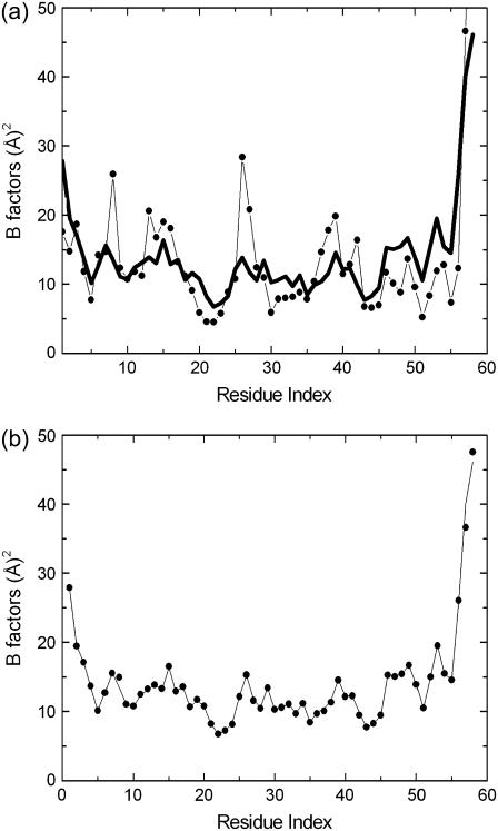
In Fig. 1 a, predictions of GNM are compared with experimental B factors. Although the fluctuation patterns of various domains are predicted well, there are significant deviations for individual residues. For example, the decrease in fluctuations in going from residue 1 to 5, the minimum about residue 10, the peak about residue 15, the minimum about residue 20, the peak around residue 40, and the two peaks around residues 48 and 54 are all predicted. However, individual peaks at residues 8, 14, 21, 26, 30, 38, 42, 47, 51, and 55 exhibit significant deviations from experiment. Normal mode decomposition of fluctuations to investigate structure-function relations, as have been the common practice in interpreting the GNM results, is most satisfactory in the low frequency modes relating to the domain motions. For the higher modes to be meaningful, precise agreement between experiment and theory is needed. This is established with the present model. In Fig. 1 b the agreement of the results of the model and experiment are clearly seen.

FIGURE 1.

(a) Experimental B factors for BPTI (thick curve) compared with the GNM prediction (light curve and solid circles), (b) Experimental B factors (light curve), which are in agreement with calculated values (solid circles).

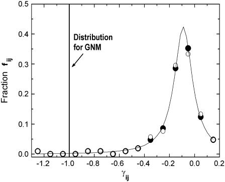
The spring constants are all equal in the GNM model, hence their distribution is a spike at −1. The present model transforms this distribution into a single-peaked Lorentzian. This is elucidated in Fig. 2. The ordinate in the figure shows the range of γ-values obtained as a result of the iterative procedure of the present model. The negative values correspond to attractive forces between the corresponding residues. The ordinate represents the fraction of the γ_ij-values corresponding to the indicated values of the abscissa. Some of the spring constants are positive, indicating repulsive forces between residue pairs that are spatially too close to each other. This last statement will be further discussed below. The solid curve is the best fitting Lorentzian that has the equation

(14)

where f_ij is the fraction of γ_ij-values, and the parameters A, γ_c, and ω are obtained for the fit shown in Fig. 2 as A = 0.426, γ_c = −0.0887, and ω = 0.174. Thus, the single peak at γ_ij = −1.0 for the GNM is now shifted to γ_c = −0.0887, and the distribution is slightly diffused around this value as seen in the figure. Calculations for several other proteins along the same lines also transform the spring constant distribution into a Lorentzian. The Lorentzians for all the proteins studied may be superposed into a single curve with proper scaling. A detailed analysis of this feature is in progress in our lab.

FIGURE 2.

The fraction of γ_ij-values obtained as a result of the present iterative model.

The distribution shown in Fig. 2 is obtained by randomly choosing a residue and modifying its interactions with all of its neighbors. The set of spring constants obtained in this manner should be independent of the random choice of the residues. The solid points in Fig. 2 show results obtained with another initial choice of the spring constants. Only those points that exhibit sufficient deviation from the original distribution are visible as solid points in the figure, the others being essentially identical and masked by the original open circles. The values of γ_ij are presented in Table 1.

TABLE 1.

Calculated values of the spring constants

Residues	Value	Residues	Value	Residues	Value
Asn24-Ala27	−1.090	Cys5-Tyr23	−0.122	Tyr23-Gln31	−0.047
Asn24-Gly28	−0.683	Ser47-Asp50	−0.119	Asp50-Arg53	−0.046
Ala16-Gly37	−0.482	Tyr21-Phe45	−0.119	Cys30-Ala48	−0.044
Ala25-Gly28	−0.453	Arg17-Tyr35	−0.118	Phe22-Thr32	−0.044
Phe4-Arg42	−0.389	Tyr10-Ala40	−0.118	Arg20-Phe45	−0.042
Ala16-Gly36	−0.338	Phe22-Asn44	−0.117	Tyr21-Cys51	−0.039
Ile18-Gly37	−0.325	Pro9-Phe22	−0.113	Tyr23-Cys55	−0.032
Asn24-Cys30	−0.315	Ile19-Tyr35	−0.111	Tyr21-Ser47	−0.028
Cys14-Gly37	−0.304	Arg20-Tyr35	−0.110	Tyr10-Lys41	−0.019
Asn24-Gln31	−0.296	Asp3-Leu6	−0.110	Phe22-Cys30	−0.016
Cys14-Cys38	−0.279	Ile18-Val34	−0.107	Lys15-Gly37	−0.016
Ile18-Tyr35	−0.276	Arg20-Phe33	−0.105	Arg20-Asn44	−0.015
Pro13-Gly36	−0.261	Ala48-Met52	−0.104	Arg1-Cys55	−0.013
Tyr10-Tyr35	−0.244	Phe22-Asn43	−0.099	Gly12-Ala40	−0.012
Gly12-Cys38	−0.226	Phe22-Phe45	−0.096	Phe22-Gln31	−0.011
Phe45-Cys51	−0.211	Tyr21-Thr32	−0.095	Tyr21-Ala48	−0.007
Pro9-Asn43	−0.210	Ile19-Phe33	−0.095	Tyr21-Gln31	−0.004
Thr11-Tyr35	−0.194	Glu49-Met52	−0.093	Arg20-Thr32	−0.003
Pro2-Cys5	−0.193	Pro2-Cys55	−0.090	Ile19-Val34	−0.002
Gly28-Gly56	−0.190	Cys30-Cys51	−0.089	Phe4-Asn43	0.011
Asn24-Leu29	−0.188	Cys51-Cys55	−0.089	Glu49-Arg53	0.014
Cys5-Asn43	−0.174	Gly12-Gly36	−0.086	Tyr21-Cys30	0.021
Ala48-Cys51	−0.164	Cys5-Cys55	−0.085	Tyr21-Lys46	0.021
Cys14-Gly36	−0.161	Cys5-Ala25	−0.084	Arg17-Val34	0.024
Ala40-Asn44	−0.154	Met52-Cys55	−0.083	Ile19-Thr32	0.028
Ile18-Gly36	−0.152	Tyr21-Asn44	−0.080	Thr11-Val34	0.028
Ser47-Cys51	−0.146	Thr11-Gly36	−0.072	Arg20-Val34	0.041
Tyr21-Phe33	−0.139	Leu6-Ala25	−0.066	Arg20-Lys46	0.050
Gly12-Tyr35	−0.138	Lys41-Asn44	−0.059	Met52-Gly56	0.060
Phe22-Phe33	−0.136	Cys30-Met52	−0.059	Tyr23-Leu29	0.072
Phe45-Asp50	−0.135	Phe22-Cys51	−0.058	Phe4-Glu7	0.103
Cys51-Thr54	−0.131	Asp50-Thr54	−0.056	Lys15-Gly36	0.107
Tyr23-Cys30	−0.124	Arg1-Cys5	−0.051	Ala25-Leu29	0.112
Tyr23-Cys51	−0.122	Arg17-Gly36	−0.049	Gly12-Arg39	0.113
Tyr23-Asn43	−0.122	Glu7-Asn43	−0.049	Arg53-Gly56	0.193

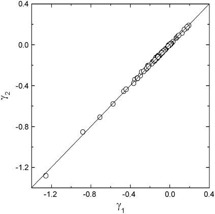
In Fig. 3 we compare the γ-values obtained by two different iterations. The random numbers used for choosing the residue pairs in the calculations were different in the two sets. The abscissa and ordinate labeled as γ₁ and γ₂, respectively, indicate the two sets of the parameters γ_ij obtained by the two independent runs. The points collapse perfectly on a 45° line that passes though the origin, indicating that the scheme is independent of the randomness inherent in the Monte Carlo scheme employed.

FIGURE 3.

Comparison of the calculated spring constants γ_ij for two different Monte Carlo runs.

The dominant factor that leads to the Lorentzian distribution shown in Fig. 2 is the average number, n_ij, of residues in the domains of fluctuation of the residues i and j, defined as

(15)

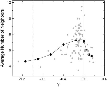
where n_i is the number of neighbors of residue i. In Fig. 4, the average number of residues n_ij are presented as a function of γ_ij. The shaded circles are obtained by counting the number of neighbors n_i and n_j that are within a cutoff distance of 7 Å of residue i and j, respectively, and using Eq. 15. The vertical dotted line shows the values of γ for the GNM and is draw for reference. The solid vertical line locates the zero of γ and is drawn to guide the eye. The average number of junctions obtained by using Eq. 15 varies between 4 and 12. The calculated values of γ_ij are shifted to larger values, but still mostly negative, indicating that the attractive forces between pairs of residues are diminished relative to that of GNM. There are, however, few positive values that represent repulsive forces between pairs. Pairs of residues in crowded environments represented by large values of n_ij correspond to small values of γ_ij. Stated in another way, these pairs are weakly connected to each other. The solid circles are obtained by averaging the values of n_ij in a given interval of γ_ij. For negative values of γ_ij, averaging is done over equal intervals of 0.25. For positive values of γ_ij, the interval is taken as 0.05 since there are fewer points in the positive region and their range is smaller. The line connects the solid points to guide the eye. The peak of the curve representing the averages is ∼γ = −0.1.

FIGURE 4.

Relationship of γ_ij-values on the average number of neighbors of residues i and j.

The present model is applied to 12 different proteins of different sizes (B. Erman, unpublished) and the magnitudes of attractive spring constants are observed to scale as

(16)

where m is in the order of 1.6 and is the mean-square fluctuation of the distance between the i^th and j^th residues, defined in terms of the mean-square residue fluctuations as

(17)

The value of is affected by two factors: First, if the mean-square fluctuations of the residues are small, then will be small, leading to a large value of the spring constant. Thus, residues in crowded regions where are small, are joined by stiffer spring constants. Secondly, for residues in less crowded regions, for anticorrelated fluctuations, the dot product in the middle term in Eq. 17 will be negative and consequently will be large, leading to a small value of γ_ij. For correlated motions, the dot product will be positive, and may be small, leading possibly to a large value of the spring constant.

With the expectation of decreasing the scatter in the calculated shaded points in Fig. 4, another run was made where the starting γ_ij-values were not equated to −1 at the outset but their values were assigned according to 1/2n_ij. At the end of the iterations, the values of γ_ij-values satisfied the 45° relation of Fig. 3. This shows that 1), the computational scheme is robust; and 2), there is an underlying effect that consistently leads to a unique set of γ_ij-values.

Effects of binding on fluctuations

A unique set of spring constants for a protein that gives a precise description of fluctuations may suitably be used for the investigation of binding effects on them. Binding of a ligand on a single residue, say i^th, has the effect of increasing the number of neighbors in the domain of fluctuation of the residue. This changes the number n_ij, thereby affecting the fluctuations of the j^th residue, and the effect propagates throughout the protein. For some residues, this effect may propagate further into the protein and for others it may die out fast. To describe and study these effects, a detailed and a precise Hamiltonian is needed and the present method of improved Γ matrix is suitable for this. Without an accurate description of fluctuations, changes caused in them by binding can only be studied qualitatively and only in the slow modes. In this section, we formulate the GNM with binding and apply it to the analysis of ligand binding on various residues of BPTI.

Binding of a ligand on a single residue

We assume that a ligand binds on the i^th residue of a protein of n residues. The Γ matrix of the new system, i.e., the protein plus the ligand, will be

(18)

The value of γ_i,n+1 measures the strength of binding of the ligand to the residue. A value of −1 makes it equivalent to a covalent bond. In the calculations below, we adopt this value.

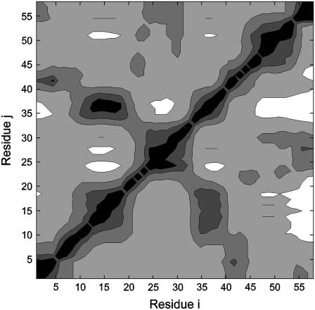
In Fig. 5, we show the changes in the fluctuations of residue j when a ligand binds on ligand i. The solid and dark-shaded contour regions indicate a decrease of fluctuations of the corresponding residues j, and the open and light-shaded regions indicate an increase. For example, binding on residue 15 decreases the fluctuations of residue 37 that falls in the solid contour. The solid regions indicate a decrease of the indicated residues along the ordinate by 3–5% relative to the unbound state. The open regions indicate an increase of fluctuations by 1–2%. The contours indicate a strong symmetry with respect to exchange of axes. This shows that the effect on residue j when binding is on residue i is similar to the effect on residue i when binding is on residue j. Response of residues to perturbation has previously been formulated and analyzed for several proteins (14–16).

FIGURE 5.

Contour map of perturbation of a residue j when binding takes place on a residue i.

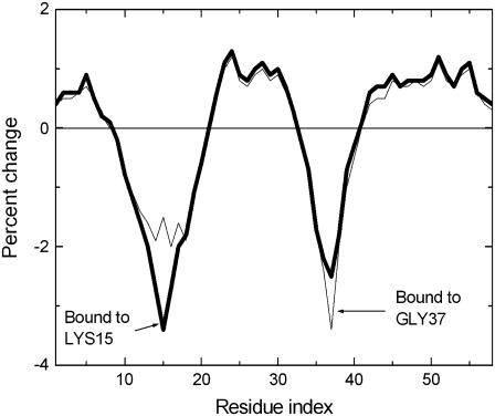
In Fig. 6, effects of binding on Lys¹⁵ and Gly³⁷ are compared. The solid curve shows the percent change in the fluctuations of other residues when binding is on residue Lys¹⁵. The fluctuations of the residues 9–20 decrease upon this binding. Also, the fluctuations of Gly³⁷ are decreased significantly, as observed from the second minimum in the solid curve. Binding also increases the fluctuations of some residues, specifically, those of 21–33 and 41–58. It is to be noted that the decrease in fluctuations of Gly³⁷ is a direct consequence of the fact that Lys¹⁵ and Gly³⁷ are close spatial neighbors. The thin line shows the changes taking place when a ligand binds on Gly³⁷. Thus the effects induced by binding on Gly³⁷ are similar to those of binding on Lys¹⁵, indicating the approximate reciprocity of binding to Lys¹⁵ and Gly³⁷.

FIGURE 6.

Binding on Lys¹⁵ and on Gly³⁷, separately.

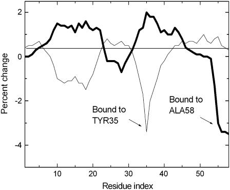
When the two residues are not neighbors in space, binding on one effects the fluctuations of the other, but the reciprocity stated above does not necessarily hold. As an example, in Fig. 7, effects of binding on residues Tyr³⁵ and Ala⁵⁸ are shown. Binding on Tyr³⁵ and Ala⁵⁸ is indicated by the thin and thick lines, respectively. Binding on Ala⁵⁸ induces an increase in the fluctuations of Tyr³⁵, but binding on Tyr³⁵ does not have any effect on the fluctuations of Ala⁵⁸. Furthermore, binding on Ala⁵⁸ induces an increase in the fluctuations of residues 8–21, whereas binding on Tyr³⁵ induces a decrease of fluctuations for these residues.

FIGURE 7.

Comparison of the effects of binding on Tyr³⁵ and Ala⁵⁸.

Binding to multiple sites on the protein

The Γ matrix defined by Eq. 16 may be extended to the case of multiple binding to different residues of a protein. For a protein of n-residues and a ligand that binds to m-sites, Eq. 16 may be written in block form as

(19)

Here, [σ]_n,m is the matrix that has n-rows and m-columns defined as

(20)

The matrix [γσ]_m,m has the form

(21)

where m-bindings have taken place on residues i, j, k, … , p, q, r. The ligand is assumed to constitute a linear chain of m-binding sites, and the linear connectivity is acknowledged by −1 values along the first off-diagonal terms of [σγ]_m,m.

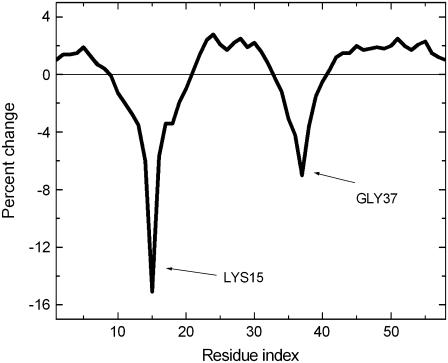
In Fig. 8, the effects of simultaneous binding on Lys¹⁵ and Gly³⁷ are shown. Compared to Fig. 6, binding simultaneously on both of these residues causes a fourfold-larger decrease than if binding took place on Lys¹⁵ only, or Gly³⁷ only.

FIGURE 8.

Binding on Lys¹⁵ and Gly³⁷.

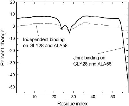
The effects of binding two independent ligands to two residues are significantly different than when the two ligands are connected to form a single molecule. In Fig. 9, effects of simultaneous and independent binding on Gly²⁸ and Ala⁵⁸ are compared. The two residues are 7.1 Å apart, and hence not within the cutoff distance of 7.0 Å.

FIGURE 9.

Effects of simultaneous binding on Gly²⁸ and Ala⁵⁸.

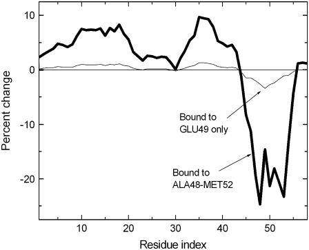
The thin line represents the effects when the spring constant between the two ligands are taken as 0 that corresponds to independent binding, i.e., two independent ligands binding on these two sites. The heavy solid curve is obtained when this spring constant between the two ligands is equated to −1. This makes the ligand behave as a single entity of two binding sites. The fluctuations of Gly²⁸ are not affected much upon this modification of the ligand. However, the fluctuations of Ala⁵⁸ are significantly reduced, and the fluctuations of the rest of the protein between residues 1–23 and 29–52 increase significantly. In Fig. 10, effects of binding at five points on the helix Ser⁴⁷-Gly⁵⁶ are shown by the solid curve. The light-shaded curve indicates effects of binding to only one residue, Glu⁴⁹, on the helix. Comparison of the two curves shows the magnification of the effect of simultaneous binding on several successive residues. The figure also shows the allosteric effects of binding, according to which binding on one part induces strong changes on another part of the protein that is far from the binding site.

FIGURE 10.

Binding on Ala⁴⁸-Met⁵² of the helix.

DISCUSSION AND CONCLUSION

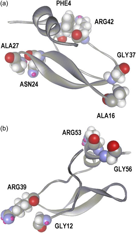
This article consists of two parts. In the first part, the originally proposed GNM is modified to obtain an exact match between experimental and predicted values of residue fluctuations. This improvement in the model is important because it provides an exact description of fluctuations in a consistent way, with the aid of which residue-specific events relating to fluctuations can be analyzed in greater detail and accuracy. The second part of the article involves the application of the model to a specific protein. In this part, we showed that an accurate description of fluctuations is indeed useful in understanding the detailed behavior of the protein. A wide range of properties of proteins relating to fluctuations have been addressed successfully with the original version of the GNM, which showed remarkable agreement with experiment at the coarse-grained level. The improvement introduced here allows for the analysis of specific details very accurately at the residue level. Corrections to an already successful model have to be justified carefully. First, it should be robust, which in turn requires the model to yield the same results irrespective of the initial distribution of γ_ij. This has been shown to be the case for BPTI. Calculations carried out on several other proteins but not reported here also show that the γ_ij-values converge to a fixed distribution, irrespective of the starting distribution of γ_ij-values. A few patterns on the magnitudes of γ_ij-values may be extracted from the results on BPTI. Firstly, the distribution of γ_ij-values obey a Lorentzian distribution, which has a pronounced peak at the small value of −0.088 (compared to −1 of GNM), and there are a few positive γ_ij-values. The repulsive springs are required in the cases where a cluster of neighboring attractive springs tend to bring certain pairs of residues close to each other, and the repulsive springs are needed to prevent the collapse of these residues onto each other. Examples of this are given below. It is to be noted that the number and strength of the repulsive springs are much smaller than those that would possibly lead to the instability of the protein. Calculations were carried out by allowing only attractive springs and equating the spring constant to zero when the simulation indicated a repulsive spring. However, convergence of the calculated fluctuations to the experimental ones was not possible in that case, and the model was not accurate. Residue pairs that have fewer neighbors are located at the surface. These are the important residue pairs in the sense that the absolute values of their γ_ij-values are large. These pairs are either strongly attracted together (pairs connected with a stiff attractive spring, or high negative value of γ_ij) or repel each other strongly (pairs connected with a stiff repulsive spring, or high positive value of γ_ij). An analysis of the spring constants given in Table 1 shows that the locations of these residues are important for the stability and/or function of the protein. For example, the largest value γ_ij = −1.09 is for the pair Asn²⁴-Ala²⁷, both of which are located on a tight turn at the surface. The next important pair is also on the same tight turn, Asn²⁴-Gly²⁸ with γ_ij = −0.68. The pair Ala¹⁶-Gly³⁷ with γ_ij = −0.48 joins the turns of two major loops at the surface of the protein. Phe⁴-Arg⁴² pair with the next highest γ_ij = −0.389 is also located at the center, joining the tail of the chain to a point on the body. The locations of these important interactions are presented in Fig. 11 a. The pair Arg⁵³-Gly⁵⁶ with the highest positive γ_ij = 0.193 is located at the end of the chain, where Gly⁵⁶ is on the free unstructured tail of the helix. Arg⁵³ is situated on the helix. The repulsive spring prevents Gly⁵⁶ from collapsing on the helix and keeps it protruding out from the surface. Similarly, each residue of the pair Gly¹²-Arg³⁹ with γ_ij = 0.113 is on the surface and located at the midpoints of the two neighboring long coils of the protein. The repulsive spring between them keeps the two coils from collapsing onto each other.

FIGURE 11.

(a) Pairs with large attractive spring constants. (b) Pairs with large repulsive spring constants.

The locations of these pairs on the surface of the protein are shown in Fig. 11 b. These examples indicate that the factors affecting the magnitudes of the spring constants depend on diverse structural features of the molecule probably relating to stability and simultaneously to function. However, inspection of Fig. 4 shows that the majority of γ_ij-values lie in a narrow region ∼γ_ij = −0.088. The outliers are those pairs at the surface of the protein.

The present model describes the fluctuations of residues in more detail than the standard GNM. To clarify the predictions of the present model relative to those of the standard GNM, we conducted a detailed modal decomposition of the present model according to the expression (17)

(22)

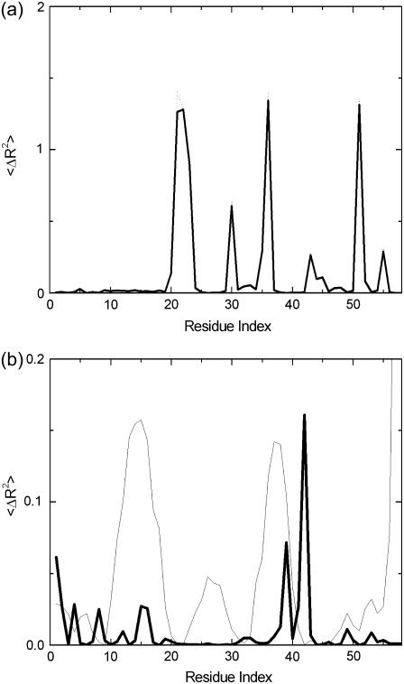
Here, denotes the k^th component of the fluctuation of the i^th residue, λ_k is the k^th eigenvalue, and [u_k]_i is the i^th component of the k^th eigenvector. In Fig. 12 a, the collective contribution of the lowest five modes is shown. The dotted line is for the standard GNM, and the solid curve is for the present model, and the two agree more or less perfectly in the lowest five cumulative modes. Fig. 12 b compares the highest five modes of the two models. Here, the thick solid line refers to the present model and the thin line to the standard GNM, and significant detail is observed in the present model while it is not present in the standard GNM. Specifically, the latter predicts a peak for the range of residues 33–42, as observed from Fig. 12 b, but the present model resolves this peak to a peak at Arg³⁹ and Arg⁴², the two important residues of the binding site. Similarly, the standard GNM gives a diffused peak in the range of residues 9–20, whereas the present model points to the significance of residues 12, 15, 16, and 19 in this range. We therefore conclude that the present model is more detailed and more specific in the higher modes. The relevance of this detail to known experimental data for different systems is the subject of future work.

FIGURE 12.

(a) Contribution of the lowest five modes to the fluctuations of residues. Solid line shows results of the present model; dotted line that of the standard GNM. (b) Contribution of the highest five modes. Thick solid line, present model; thin solid line, standard GNM.

Finally, it is worthwhile to add several recently published articles relating to research reported in this article; for example, Ming and Wall (18), who improved the model by strengthening backbone interactions; Tobi and Bahar (19), who found correlations between intrinsic motions of unbound proteins and structural changes upon binding; and Sen et al. (20), who systematically compared Gaussian Network Models with varying scales of coarse-graining.

References

- 1.Bahar, I., A. R. Atilgan, and B. Erman. 1997. Direct evaluation of thermal fluctuations in proteins using a single-parameter harmonic potential. Fold. Des. 2:173–181. [DOI] [PubMed] [Google Scholar]
- 2.Kloczkowski, A., J. E. Mark, and B. Erman. 1989. Chain dimensions and fluctuations in random elastomeric networks. I. Phantom Gaussian networks in the undeformed state. Macromolecules. 22:1423–1432. [Google Scholar]
- 3.Erman, B., and P. J. Flory. 1982. Relationship between stress, strain, and molecular constitution of polymer networks. Comparison of theory with experiments. Macromolecules. 15:806–812. [Google Scholar]
- 4.Tirion, M. M. 1996. Large amplitude elastic motions in proteins from a single-parameter atomic analysis. Phys. Rev. Lett. 77:1905–1908. [DOI] [PubMed] [Google Scholar]
- 5.Bahar, I., A. R. Atilgan, M. C. Demirel, and B. Erman. 1998. Vibrational dynamics of folded proteins: significance of slow and fast motions in relation to function and stability. Phys. Rev. Lett. 80:2733–2736. [Google Scholar]
- 6.Bahar, I., B. Erman, R. L. Jernigan, A. R. Atilgan, and D. G. Covell. 1999. Collective motions in HIV-1 reverse transcriptase: examination of flexibility and enzyme function. J. Mol. Biol. 285:1023–1037. [DOI] [PubMed] [Google Scholar]
- 7.Halle, B. 2002. Flexibility and packing in proteins. Proc. Natl. Acad. Sci. USA. 99:1274–1279. [DOI] [PMC free article] [PubMed] [Google Scholar]
- 8.Micheletti, C., J. R. Banavar, and A. Maritan. 2001. Conformations of proteins in equilibrium. Phys. Rev. Lett. 87:8102–8105. [DOI] [PubMed] [Google Scholar]
- 9.Kundu, S., J. S Melton, D. C Sorensen, G. N. Phillips. 2002. Dynamics of proteins in crystals: comparison of experiment with simple models. Biophys. J. 83:723–732. [DOI] [PMC free article] [PubMed] [Google Scholar]
- 10.Ming, D., Y. Kong, M. A. Lambert, Z. Huang, and J. Ma. 2002. How to describe protein motion without amino acid sequence and atomic coordinates. Proc. Natl. Acad. Sci. USA. 99:8620–8625. [DOI] [PMC free article] [PubMed] [Google Scholar]
- 11.Moritsugu, K., O. Miyashita, and A. Kidera. 2000. Vibrational energy transfer in a protein molecule. Phys. Rev. Lett. 85:3970–3973. [DOI] [PubMed] [Google Scholar]
- 12.Moritsugu, K., O. Miyashita, and A. Kidera. 2003. Vibrational energy transfer in a protein molecule. J. Phys. Chem. B. 107:3309–3317. [DOI] [PubMed] [Google Scholar]
- 13.Reference deleted in proof.
- 14.Yilmaz, L. S., and A. R. Atilgan. 2000. Identifying the adaptive mechanism in globular proteins: fluctuations in densely packed regions manipulate flexible parts. J. Chem. Phys. 113:4454–4464. [Google Scholar]
- 15.Baysal, C., and A. R. Atilgan. 2001. Elucidating the structural mechanisms for biological activity of the chemokine family. Proteins. 43:150–160. [DOI] [PubMed] [Google Scholar]
- 16.Baysal, C., and A. R. Atilgan. 2001. Coordination topology and stability for the native and binding conformers of chymotrypsin inhibitor 2. Proteins Struct. Funct. Gen. 45:62–70. [DOI] [PubMed] [Google Scholar]
- 17.Demirel, M. C., A. R. Atilgan, R. L. Jernigan, B. Erman, and I. Bahar. 1998. Identification of kinetically hot residues in proteins. Protein Sci. 7:2522–2532. [DOI] [PMC free article] [PubMed] [Google Scholar]
- 18.Ming, D., and M. E. Wall. 2005. Allostery in a coarse-grained model of protein dynamics. Phys. Rev. Lett. 95:198103–198106. [DOI] [PubMed] [Google Scholar]
- 19.Tobi, D., and I. Bahar. 2005. Structural changes involved in protein binding correlate with intrinsic motions of proteins in the unbound state. Proc. Natl. Acad. Sci. USA. 102:18908–18913. [DOI] [PMC free article] [PubMed] [Google Scholar]
- 20.Sen, T. Z., Y. Feng, J. V. Garcia, A. Kloczkowski, and R. L. Jernigan. 2006. The extent of cooperativity of protein motions observed with elastic network models is similar for atomic and coarser-grained models. J. Chem. Theory Comput. 2:696–704. [DOI] [PMC free article] [PubMed] [Google Scholar]