Theoretical Accuracy of Model-Based Shape Matching for Measuring Natural Knee Kinematics with Single-Plane Fluoroscopy

Abstract

Quantification of knee motion under dynamic, in vivo loaded conditions is necessary to understand how knee kinematics influence joint injury, disease, and rehabilitation. Though recent studies have measured three-dimensional knee kinematics by matching geometric bone models to single-plane fluoroscopic images, factors limiting the accuracy of this approach have not been thoroughly investigated. This study used a three-step computational approach to evaluate theoretical accuracy limitations due to the shape matching process alone. First, cortical bone models of the femur, tibia/fibula, and patella were created from CT data. Next, synthetic (i.e., computer generated) fluoroscopic images were created by ray tracing the bone models in known poses. Finally, an automated matching algorithm utilizing edge detection methods was developed to align flat-shaded bone models to the synthetic images. Accuracy of the recovered pose parameters was assessed in terms of measurement bias and precision. Under these ideal conditions where other sources of error were eliminated, tibiofemoral poses were within 2 mm for sagittal plane translations and 1.5 deg for all rotations while patellofemoral poses were within 2 mm and 3 deg. However, statistically significant bias was found in most relative pose parameters. Bias disappeared and precision improved by a factor of two when the synthetic images were regenerated using flat shading (i.e., sharp bone edges) instead of ray tracing (i.e., attenuated bone edges). Analysis of absolute pose parameter errors revealed that the automated matching algorithm systematically pushed the flat-shaded bone models too far into the image plane to match the attenuated edges of the synthetic ray-traced images. These results suggest that biased edge detection is the primary factor limiting the theoretical accuracy of this single-plane shape matching procedure.

1 Introduction

Between 1997 and 2002, the number of Americans afflicted with arthritis more than doubled to 70 million, making arthritis the new leading cause of work disability [1]. According to the Arthritis Foundation, the most common form of arthritis, osteoarthritis (OA), appears in the knee more than any other joint. Disease development and progression are influenced by abnormal joint kinematics under dynamic, weight-bearing conditions [2,3]. Therefore, knowledge of kinematics in healthy and arthritic knees would be extremely valuable for understanding the disease’s etiology and predisposing factors as well as for guiding surgical planning, technique, and procedure.

Few studies have measured three-dimensional (3D) knee kinematics under loaded, physiological conditions with submillimeter accuracy as needed to study arthritis-related issues. Video-based motion analysis with surface markers has been used widely to study gross body motion but less to study detailed joint motion due to the problem of skin and soft tissue motion artifacts [4–10]. Use of redundant surface markers to correct for motion artifacts shows promise and evaluation of these methods is ongoing [9,10]. However, the most direct way to eliminate these issues is to measure joint motion using x-ray techniques. For artificial knees, single-plane fluoroscopy has been used to measure implant motion directly [11–15]. With this approach, 3D computer aided design (CAD) models of the metallic components are aligned to each 2D fluoroscopic image to quantify pose (translation and rotation) parameters. This approach works well since the metallic components have precisely known geometric features and produce sharp edges in fluoroscopic images. For natural knees, since CAD models of the bones are not readily available from the manufacturer, biplane fluoroscopy with implanted bone markers has been used instead [16–18]. Though more accurate than single-plane fluoroscopy, this approach requires surgical implantation of metal beads which restricts its use to research projects with limited populations.

Building on the example of artificial knee studies, researchers have recently begun to use single-plane fluoroscopy to measure natural knee motion [19–21]. For the shape matching procedure, implant CAD models are replaced with geometric bone models created from medical imaging data. However, in fluoroscopic images, cortical bone edges are less well defined than are metallic implant edges [16]. Consequently, to evaluate the extent to which this approach can be used to study arthritis-related issues, a theoretical accuracy assessment is needed to quantify expected errors in measured joint (relative) and bone (absolute) kinematics.

This study quantifies relative and absolute accuracy limitations due to the shape matching process alone when natural knee kinematics are measured by aligning flat-shaded, edge detected bone models to single plane fluoroscopic images. Similar to the approach used for knee implant components, flat shading is used in the shape matching process due to the high computational cost of repeatedly ray tracing the bone models in different trial poses. The four specific goals were: (1) to generate synthetic fluoroscopic images by ray tracing the bone models in known poses, (2) to develop an automated matching algorithm that finds relative and absolute bone model pose parameters consistent with the synthetic images, (3) to assess the procedure under conditions in which all sources of experimental error are eliminated except those related to image generation and shape matching, and (4) to evaluate the extent to which bone edge attenuation in images degrades the accuracy of the measurements. These results help define the theoretical capabilities and limitations of the proposed single-plane shape matching procedure and provide a bound on the best possible accuracy one can hope to achieve with this approach.

2 Methods

A three-step computational approach was used to quantify the accuracy with which edge-detected bone models can be matched to single-plane fluoroscopic images of the knee. First, geometric cortical bone models were created from CT data. Next, synthetic (i.e., computer-generated) fluoroscopic images were created with the bone models in known poses. Finally, an automated matching algorithm was developed to align the bone models to the synthetic images. Though the methodology described here is tailored to accuracy assessment of synthetic images, it can also be used to measure in vivo bone motion from single-plane fluoroscopic images.

2.1 Bone Model Creation

Geometric cortical bone models of the femur, tibia/fibula, and patella were created from CT scan data for synthetic image generation and automated shape matching. One healthy subject gave informed consent to undergo fine and coarse axial CT scans of the left leg as approved by the institutional review board. Both scans used a 512×512 image matrix with a pixel size of 0.39×0.39 mm [Fig. 1(a)]. The fine scan used 1.25 mm slices spanning approximately 75 mm above and below the joint line of the knee, while the coarse scan used 5 mm slices from the hip center to the ankle center. This approach minimized subject radiation exposure while obtaining accurate geometric information in the knee region [20]. Interior and exterior cortical bone edges for the femur, tibia, fibula, and patella were segmented using a commercial watershed algorithm (Slice-Omatic, Tomovision, Montreal, CA) [Fig. 1(b)], and points defining the segmented outlines of cortical bone [Fig. 1(c)] were exported by the software. The segmentation process was semi-automatic, requiring user intervention only for slices near the ends of the bones where volume averaging effects make edge detection more difficult.

Fig. 1.

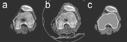
Segmentation of CT data to generate point clouds for geometric cortical bone models. (a) Sample CT image of the femur and patella. (b) Boundaries identified by the watershed algorithm. (c) Cortical bone contours defined from the segmentation.

The point clouds resulting from the segmentation process [Fig.2(a)] were converted into polygonal surface models using commercial reverse engineering software (Geomagic Studio, Raindrop Geomagic, Research Triangle Park, NC). Polygonal surfaces were fitted automatically by the software to each fine and coarse point cloud. The coarse polygonal models were then aligned to their fine counterparts using the software’s three-dimensional automatic alignment algorithm. Alignment was performed only for the femur and tibia/fibula. For the patella, the fine model was used directly. Coarse model polygons in the fine scan region were deleted and the gap between fine and coarse models filled automatically. To create uniform polygon density, all polygons were subdivided and then decimated back to the original number of polygons using the software’s curvature-based decimation algorithm [Fig. 2(b)]. The final bone models were created by boolean subtraction and contained the interior and exterior cortical bone surfaces [Fig. 2(c)]. The tolerance between the final polygonal surfaces and original point clouds was an average of 0.15 mm over all surfaces of all bones with a standard deviation of 0.12 mm.

Fig. 2.

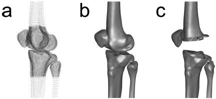
Creation of polygonal cortical bone models from the point cloud data. (a) Segmented point clouds demonstrating the outer and inner cortical bone boundaries as well as the regions covered by the fine and coarse scans. (b) Polygonal surface models fitted to the point clouds using commercial reverse engineering software. (c) Cutaway view of polygonal models showing the outer and inner cortical surfaces of each bone.

In preparation for fluoroscopic shape matching, anatomic coordinate systems were created in each bone model following an approach similar to previous studies [17,18]. The mechanical axis of the leg, as determined from CT slices through the hip and ankle centers, was used to define the superior–inferior axis for the femur and the tibia/fibula. The medial–lateral axis of the femur was de-fined by the transepicondylar axis and of the tibia/fibula by the line connecting the most medial and lateral points on the tibial plateau. The third axis was formed from the cross product of the first two. The coordinate system origin of the femur was defined as the midpoint of the transepicondylar line, while the origin of the tibia/fibula was defined as the centroid of the tibial plateau located at the level of the articular surfaces. The patella coordinate system was identical to that of the tibia/fibula with the knee as scanned in full extension. Relative translation and rotation between the tibia and fibula were assumed to be negligible, and the two models were combined into one for shape matching purposes [20].

2.2 Synthetic Image Creation

Once the bone models were developed, synthetic (i.e., computer-generated) fluoroscopic images were created with the bone models in known poses. Three sets of synthetic image sets were analyzed: (1) images replicating an in vivo stair rise motion created using ray tracing with a bone transparency coefficient of 1.0 (completely transparent) and attenuation coefficient of 0.999 (high attenuation), (2) similar ray-traced images where the three bone models were randomly transformed as a single rigid body, and (3) flat-shaded images identical to the second sequence. Similar to the experimental conditions for the first set, approximately 30 synthetic images were generated for each of the three image sets.

The first synthetic image set used ray-tracing to evaluate relative and absolute measurement errors under conditions that simulated an in vivo, loaded experimental situation [18]. The same subject who provided the CT data gave informed consent to perform a stair rise activity under fluoroscopic analysis using a protocol approved by the institutional review board [Fig. 3(a)]. Images were collected at 30 frames/s producing approximately 30 frames for each of three trials. Bone models of the femur, tibia/ fibula, and patella were manually aligned to the fluoroscopic images from one of the trials using custom software [Fig. 3(b)][12]. Patellar poses were not calculated for images where the patella moved outside of the field of view (13 images). Pose parameters found for one frame seeded the initial guess for the subsequent frame, where rotational pose parameters were calculated using the convention of Tupling and Pierrynowski [22].

Fig. 3.

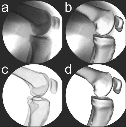
Synthetic fluoroscopic image creation process to simulate an in vivo stair rise motion. (a) Sample experimental fluoroscopic image. (b) Femur, tibia/fibula, and patella bone models manually matched to the experimental image. (c) orresponding synthetic fluoroscopic image generated by ray tracing the cortical bone models in their manually matched poses. (d) Femur, tibia/fibula, and patella bone models automatically matched to the synthetic image to evaluate the accuracy of the recovered pose parameters.

Synthetic fluoroscopic images were created from the manually-determined experimental poses using commercial surface modeling and rendering software (Rhinoceros and Flamingo, Robert McNeel and Associates, Seattle, WA). The viewing properties were configured to produce a principal distance and image scale that matched the experimental setup, while the cortical bone models were given light attenuating material properties to produce images similar to x rays. Once the three bone models were placed in the desired pose, ray tracing was used to generate a synthetic fluoroscopic image [Fig. 3(c)] that eliminated motion blur, nonuniform image intensity, soft tissue effects, and other sources of experimental error. This process was repeated for each pose and the resulting synthetic images output to the shape matching software. An automated matching algorithm (details below) was then used to align the bone models to the synthetic images to quantify the relative and absolute errors in the recovered pose parameters [Fig. 3(d)].

The second synthetic image set tested a wider range of absolute bone poses by applying random transforms to the bone models in a fixed relative pose. A single experimental image from the first set was chosen to define realistic relative pose parameters for the three bone models [Fig. 4(a)]. Ray-tracing was used to generate synthetic images after random transformations were applied to the three bone models treated as a single rigid body [Fig. 4(b)]. This approach assured that the relative poses of the bones would be the same in all random images. The magnitudes of the uniformly-distributed random transformations were ±50 mm for all three translations, ±15 deg for the x and y (out-of-plane) rotations, and ±45 deg for the z (in-plane) rotation [11]. Random images were generated with these settings until 30 were obtained where all three bones were within the field of view. For each image, the bone models were manually placed close to their perceived best poses prior to automated matching [16,23] since random transformations do not produce images with pose continuity.

Fig. 4.

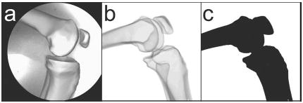
Synthetic fluoroscopic image creation process to simulate a wide array of random poses with the bone models in a fixed relative pose. (a) Experimental fluoroscopic image with manually matched bone models used to define the relative pose parameters for all random images. (b) Synthetic fluoroscopic image generated using ray tracing after application of a random transformation to the cortical bone models. (c) The same synthetic fluoroscopic image generated using flat shading instead of ray tracing to eliminate bone edge attenuation.

The third image set was identical to the second except that flat shading was used in place of ray tracing to evaluate the influence of bone edge attenuation on matching accuracy [Fig. 4(c)]. Unlike ray-traced bone images, flat-shaded images possess sharp edges similar to those of metallic implant components. Thus, flat shading eliminates bone edge attenuation visible in both synthetic ray-traced and experimental fluoroscopic images.

2.3 Automated Shape Matching

To eliminate user expertise as a confounding factor in the accuracy assessment, an automated shape matching algorithm was developed. For each bone, the general concept was to edge detect the flat-shaded bone model, then edge detect the same bone in the synthetic fluoroscopic image, and finally move the bone model until its edges best matched those in the synthetic image. For consistency, Canny edge detection was used on both the bone model and the fluoroscopic image [23]. Matching was achieved via a novel optimization procedure (details below) whose cost function minimized the normalized sum of the distances between the two sets of edge points. Distances were measured in units of pixels and calculated from image edges, which remain constant for a particular image, to bone edges, which change as the bone model pose is modified. Normalization by the number of selected image edge points was performed to make the results insensitive to this variable. Interior geometric features were not detected or used in the cost function due to the high computational cost that would be incurred by repeatedly ray tracing, instead of flat shading, each bone model. To simplify bone edge detection in each fluoroscopic image, a mask (±4−10 pixels) was placed around the edges of the bone model in its initial pose, and only those image points located within the mask were used for image edge detection.

The optimization procedure was based on a univariate search method minimizing errors in one pose parameter at a time rather than all six pose parameters simultaneously. The order in which the six pose parameters were optimized was determined by calculating the sensitivity of the cost function to changes in each pose parameter separately. The pose parameters were defined such that x and y corresponded to in-plane translations while z corresponded to out-of-plane translation measured with respect to the fixed image plane. The three most sensitive directions (in-plane pose parameters: x and y translation and z rotation) were optimized first, followed by the three least sensitive directions (out-of-plane pose parameters: x and y rotation and z translation). The entire sequence of six one-dimensional optimizations was iterated until the specified absolute or relative convergence tolerance was met.

For each one-dimensional search, a six-step curve-fitting approach was used to find the minimum. First, seven points with wide initial spacing were sampled along the search direction [Fig.5(a)]. Second, these points were resampled so that the lowest point was in the middle, shifting the sampled points in one direction or the other while maintaining the same spacing [Fig. 5(b)]. Third, a cubic polynomial, which only requires four sampled points, was fit through the seven points using linear least squares [Fig. 5(c)]. A cubic was chosen instead of a quadratic since the cost function was asymmetric about the minimum for each search direction. Fourth, the redundant points were used to assess the goodness of fit and noise present in the cubic. Goodness of fit was quantified by calculating the adjusted R² value, while noise was quantified by calculating the standard error of the estimate s. Fifth, an automatic step size adjustment algorithm was used to modify the point spacing until R² was greater than 0.99 and s was less than 1. These values were chosen empirically based on experience with the algorithm. Finally, the minimum was calculated analytically from the converged cubic curve fit.

Fig. 5.

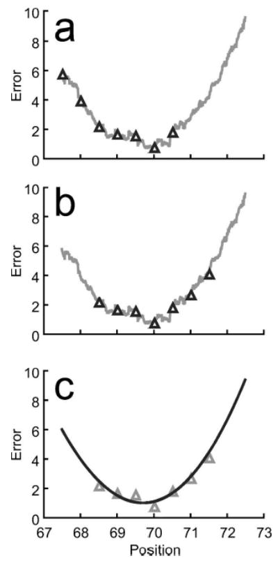
Univariate optimization using cubic curve fitting to account for noise in the cost function. (a) Example of a noisy cost function in one direction along with seven initial sampled points. (b) Shifted sampled points using the same spacing to move the lowest point to the middle. (c) Least-squares cubic curve fit of the sampled points to evaluate fit accuracy, adjust sampled point spacing if needed, and calculate the minimum analytically.

Central to this approach is the automatic step size adjustment algorithm used to produce stable and rapid convergence. Neither R² nor s alone was sufficient to identify cubic curve fits that accurately predicted the minimum. However, when R² and s information were combined, four separate combinations (or regions) were identified that could be used to guide the step size adjustment process (Fig. 6). These regions were defined as follows: Region 1—R²<0.99, s<1; Region 2—R²>0.99, s<1; Region 3—R²>0.99, s>1; Region 4—R²<0.99, s>1. The goal was to find a cubic curve fit in Region 2, where the goodness of fit was high and noise low. Once a candidate cubic fit was generated, the region was identified from the fits R² and s values. The step size was then adjusted based on the following general algorithm: Region 1, double the step size; Region 2, test for convergence; Region 3, halve the step size; Region 4, quarter the step size. If the fit lay in region 2 but did not pass the convergence test, the step size was halved. In addition, the previous region found was stored and used to make additional step size adjustments to avoid stepping over Region 2 in one direction or the other. This six-step process was iterated until the specified absolute or relative tolerance was met.

Fig. 6.

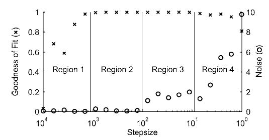
Automatic step size adjustment rationale to select sampled point spacing for an accurate cubic curve fit. Left axis is goodness of fit quantified using the adjusted R² value, while right axis is noise quantified using the standard error of the estimate s. Four potential regions can be identified by combining R² and s information: Region 1—R²<0.99, s<1; Region 2—R²>0.99, s<1; Region 3—R²>0.99, s>1; Region 4—R²<0.99, s >1. Knowledge of the region for the current fit can be used to adjust the sampled point spacing automatically (see text) until the fit is in region 2, where R² is high and s is low.

2.4 Data Analysis

The accuracy of the automated shape matching process was quantified in terms of bias and precision [11,18,23]. Bias was calculated from the mean matching error for each of the six pose parameters in each synthetic image set, while precision was calculated from the corresponding standard deviations. For bias results, a Student’s t-test (p<0.05) was performed to determine if the values were statistically different from zero, indicating the presence of a systematic error. All synthetic image generation and automated matching calculations were performed on a 1.8 GHz Pentium IV PC.

3 Results

Measurement precision for relative pose parameters for image set 1 was approximately 2 mm for sagittal plane translations and 1.5 deg for all rotations for tibiofemoral kinematics and about 2 mm and 3 deg for patellofemoral kinematics (Table 1). Measurement precision for medial-lateral translation was approximately 7 mm for tibiofemoral and 16 mm for patellofemoral kinematics. Systematic error or bias comparable in magnitude to the precision values was found in most relative pose parameters. When larger absolute motions were analyzed using image set 2, bias and precision results were generally consistent with those of image set 1. The main differences were worse sagittal plane translational precision and a decrease in varus–valgus and internal–external rotational bias. Measurement precision improved by a factor of 2 when flat shading was used in place of ray tracing for image set 3 and nearly all bias disappeared, with the one remaining bias being small (< 0.06 deg). For all three image sets, relative precisions were generally less than the sum of the closest corresponding absolute precisions (see below) with the exception of sagittal plane translations. For example, for image set 1, tibiofemoral anterior–posterior translation precision was 2.1 mm, which was greater than the sum of the femur and tibia/fibula x translation precisions of 0.27 and 0.42 mm, respectively.

Table 1.

Relative pose parameter bias±precision calculated from three synthetic fluoroscopic image sets corresponding to an in vivo experimental stair rise motion or randomly transformed bones in a fixed relative pose. Directions are with respect to the anatomic coordinate systems, where A–P is anterior–posterior, S–I is superior–inferior, M–L is medial–lateral, V–V is varus–valgus, I–E is internal–external, and F–E is flexion–extension.

Synthetic images	Pose parameters	Tibiofemoral	Patellofemoral
Set 1	A– P translation (mm)	1.5±2.1a	1.1±1.7a
Ray-Traced	S–I translation (mm)	0.84±0.52a	−0.42±0.95a
Experimental	M –L translation (mm)	7.7±7.3a	9.5±16a
	V–V rotation (deg)	0.33±1.4	−2.6±2.8a
	I–E rotation (deg)	−1.1±0.95a	1.2±2.6a
	F–E rotation (deg)	−0.051±0.49	−0.096±0.86
Set 2	A– P translation (mm)	1.0±2.1a	1.6±3.5a
Ray-Traced	S–I translation (mm)	1.1±1.9a	0.80±1.9a
Random	M –L translation (mm)	3.0±8.1a	7.2±10a
	V–V rotation (deg)	0.53±1.1a	−0.53±2.7
	I–E rotation (deg)	0.22±0.93	0.61±1.6a
	F–E rotation (deg)	−0.25±0.39a	−0.23±0.44a
Set 3	A– P translation (mm)	0.26±0.86	0.070±0.62
Flat-Shaded	S–I translation (mm)	−0.014±0.85	−0.14±0.55
Random	M –L translation (mm)	0.50±3.93	0.75±4.0
	V–V rotation (deg)	0.065±0.62	−0.28±1.3
	I–E rotation (deg)	0.098±0.50	0.37±1.8
	F–E rotation (deg)	−0.058±0.18a	−0.058±0.20

^aBias is statistically different from zero (p<0.05) based on a Student’s t-test.

Measurement precision for absolute pose parameters for image set 1 was within 0.4 mm for in-plane (x and y) translations and 1.3 deg for all rotations for the femur and fibula/tibia and 0.7 mm and 2.8 deg for the patella (Table 2). Precision for out-of-plane translations was within 6 mm for the femur and tibia/fibula and 13 mm for the patella. For all three bones, a negative statistically significant bias was present in the out-of-plane (z) translation that tended to push the bone models into the image plane. Other statistically significant biases were present but were not consistent for all three bones. When image set 2 was analyzed with a larger range of absolute motions, precision and bias results were generally consistent with those from image set 1. Significant bias for all three bones was found for the out-of-plane translation. When the image generation process was switched to flat shading for the third image set, precision results improved by roughly a factor of 2, and nearly all statistically significant biases disappeared, including all out-of-plane translation biases. The three remaining statistically significant biases were small (<0.08 mm and 0.05 deg).

Table 2.

Absolute pose parameter bias±precision calculated from three synthetic fluoroscopic image sets corresponding to an in vivo experimental stair rise motion or randomly transformed bones in a fixed relative pose. Directions are with respect to the fluoroscopic coordinate system, where x (forward) and y (upward) are parallel to the image plane and z (outward) is perpendicular to the image plane.

Synthetic images	Pose parameters	Femur	Tibia/Fibula	Patella
Set 1	X translation (mm)	−0.031±0.27	0.081±0.42	0.16±0.48
Ray-Traced	Y translation (mm)	0.043±0.28	−0.49±0.21a	0.66±0.71a
Experimental	Z translation (mm)	−3.3±5.6a	−11±5.2a	−9.8±13a
	X rotation (deg)	0.15±0.47	−0.18±1.3	−2.6±2.8a
	Y rotation (deg)	0.99±0.72a	−0.41±0.40a	2.4±2.6a
	Z rotation (deg)	−0.028±0.56	−0.065±0.22	−0.089±0.59
Set 2	X translation (mm)	0.17±0.28a	0.031±0.37	0.41±0.30a
Ray-Traced	Y translation (mm)	0.059±0.20	−0.42±0.36a	−0.045±0.42
Random	Z translation (mm)	−6.7±5.7a	−11±7.6a	−13±10a
	X rotation (deg)	−0.32±0.65a	−0.043±0.87	−1.2±2.5a
	Y rotation (deg)	0.56±0.60a	−0.14±0.65	0.60±1.6a
	Z rotation (deg)	−0.19±0.36a	0.014±0.34	−0.042±0.14
Set 3	X translation (mm)	0.037±0.16	−0.037±0.20	0.078±0.11a
Flat-Shaded	Y translation (mm)	−0.058±0.13a	0.0093±0.18	−0.021±0.34
Random	Z translation (mm)	0.57±2.3	−0.46±3.1	0.22±4.2
	X rotation (deg)	−0.14±0.47	0.028±0.45	−0.39±1.3
	Y rotation (deg)	0.060±0.29	−0.074±0.29	0.25±1.7
	Z rotation (deg)	−0.046±0.093a	−0.0012±0.14	0.0064±0.18

^aBias is statistically different from zero (p<0.05) based on a Student’s t-test

4 Discussion

This study used a computational approach to quantify the theoretical accuracy with which natural knee kinematics can be measured using single-plane fluoroscopy and flat-shaded, edge detected bone models when all sources of error are eliminated except those related to image generation and shape matching. Three-dimensional cortical bone models were created from CT scan data and ray traced to generate synthetic fluoroscopic images with the bones in known poses. An automated matching algorithm was developed to assess the theoretical accuracy with which the known pose parameters could be recovered by aligning flat-shaded bone models to the synthetic images. For synthetic images that simulated an in vivo, loaded stair rise motion, precision for tibiofemoral kinematics was 2 mm for sagittal plane translations and 1.5 deg for all rotations, while precision for patellofemoral kinematics was 2 mm and 3 deg. Medial–lateral translations were much less precise, with statistically significant bias present in nearly all relative pose parameters. Evaluation of absolute pose parameter errors in images generated using flat shading instead of ray tracing revealed that systematic out-of-plane translation errors due to bone edge attenuation were the primary source of measurement bias.

A computational rather than experimental approach was used in this study to provide a well-controlled environment for evaluating theoretical accuracy. If the accuracy determined by this method was poor, little motivation would exist for a thorough experimental evaluation. Similar errors for the two ray-traced image sets suggest that the results were reliable and representative of the accuracy that could be obtained from single-plane fluoroscopic images under ideal conditions. In experimental practice, however, additional confounding factors such as imperfect image distortion correction, motion blur due to long exposure times [16], less clear bone edges due to surrounding soft tissue [16], and imperfect bone geometric models [23] would make the accuracy worse. For example, the bone geometric models used in our shape matching process were identical to those used to generate the synthetic images, whereas in real life, bone geometric models derived from CT scan data will never be completely consistent with bone images measured using fluoroscopy. For one, CT and fluoroscopic x-ray techniques have different energy absorption and scatter characteristics. For another, CT scans do not capture bone geometry perfectly due to limited in-plane resolution, volume averaging over a finite slice thickness, imperfect segmentation of bone edges, and smoothing during polygonal surface creation. None of these sources of error were included in our analysis.

Direct comparison of our tibial and femoral precision results with those reported by other knee fluoroscopy studies is difficult due to differences in accuracy assessment methods and included sources of error. Nonetheless, comparison still provides a general sense of the extent to which bone edge attenuation may affect the overall accuracy of the measurement process (Table 3). Single-plane fluoroscopy studies of natural knees using image-matched bone models reported precision results comparable to those of our study [19,20], even though these studies used internal bone contours as well as bone edges for matching. Studies of artificial knees have reported comparable or better precision, likely due to unambiguous edge identification [11,13,15]. Bi-plane studies using implanted bone markers or implants achieved an order of magnitude improvement for all absolute pose parameters [18,23]. However, when bone models were matched to bi-plane fluoroscopic images, precision results were closer to those of our study, apart from out-of-plane translation [16]. Only two studies reported relative precision results for the tibiofemoral joint [11,15]. Those studies used single-plane fluoroscopy with implant models and reported relative rotation precisions comparable to our study and relative translation precisions that were approximately two to four times better. No other studies have reported precision results for the patella or the patellofemoral joint. High uncertainty for patellar out-of-plane rotations is consistent with limited distinguishing bone geometry.

Table 3.

Femoral and tibial absolute precision results reported by knee fluoroscopy studies in the literature

Reference	Fluoroscopy method	Knee type	Models matched	In-plane Trans (mm)	Out-of-plane trans (mm)	All rots (deg)
Present study	Single-plane	Natural	Bones	0.42	5.6	1.3
Kanisawa et al. [19]	Single-plane	Natural	Bones	1.2	4.0	0.8
Komistek et al. [20]	Single-plane	Natural	Bones	0.45	· · ·	0.66
Banks and Hodge [11]	Single-plane	Artificial	Implants	0.21	3.9	1.3
Hoff et al. [13]a	Single-plane	Artificial	Implants	0.46	2.2	0.35
Mahfouz et al. [15]	Single-plane	Artificial	Implants	0.09	1.4	0.40
Tashman et al. [18]	Bi-plane	Natural	Markers	0.06	0.06	0.31
You et al. [16]a	Bi-plane	Natural	Bones	0.23	0.23	1.2
Kaptein et al. [23]	Bi-plane	Artificial	Markers	0.05	0.08	0.07
Kaptein et al. [23]	Bi-plane	Artificial	Implants	0.06	0.14	0.17

^aRMS errors rather than precision results reported

Off-the-shelf optimization methods were not chosen for our automated matching algorithm due to the characteristics of the system being analyzed. Global optimization would have required excessive CPU time due to a large number of costly function evaluations. Gradient-based optimization was implemented but not chosen due to a discontinuous cost function in each search direction (Fig. 5). As the bone model pose was modified during gradient calculations, image edge points were compared with changing bone model edge points, producing inaccurate search directions and convergence to a local minimum. Response surface methods fitting more than one pose parameter at a time were also unsuccessful, since the noisy nature of the search space made it difficult to select the correct distance between sample points in multiple dimensions.

Attenuated bone edges appear to be the primary source of systematic error in the analysis. Elimination of large z translation bias in the flat-shaded synthetic images indicates that this bias was due to bone edge attenuation in the ray-traced synthetic images. In addition to negative z translation bias, y rotation bias was also strong though not consistent for all three bones. For the two ray-traced image sets, the femur and patella demonstrated statistically significant positive y rotation bias. In contrast, the tibia/fibula demonstrated negative y rotation bias that was statistically significant only for image set 1, where smaller out-of-plane rotations provided less y rotation information from the fibula than in image set 2. It is therefore possible that shrinking the bone model edges to accommodate edge attenuation in the ray-traced images was accomplished not only by pushing the bone models into the image plane but also by rotating them about the y axis.

The relative precision and bias results for the ray traced image sets were influenced by kinematic coupling between the absolute pose parameter errors. Based on kinematics theory, each absolute translation error can contribute to all three relative translations errors and each absolute rotation error to all six relative pose parameter errors. For example, if a 90° y axis rotation was applied to all three bones, anterior–posterior translation would now be in the z direction, which is the least precise. Thus, the worse-than-expected relative precision results for sagittal plane translations were likely due to contributions from poor z translation precision. Relative precision results for medial–lateral translation were actually better than expected since the two contributing z translation precisions were biased in the same direction, producing some cancellation of errors. Bias in nearly all relative pose parameters can be explained by contributions from z translation bias to all three relative translations and y rotation bias to all six relative pose parameters.

Although many factors contribute to inaccuracies in kinematic measurements made from single-plane fluoroscopy, this study was limited to a subset of those factors. Only one pixel size and grid were selected to represent experimental conditions. Smaller pixels with a higher resolution would likely produce more accurate results. Principle distance between the bone models and the image detector was representative of experimental conditions (1100 mm). As the principle distance decreases, the sensitivity to out-of-plane translation increases. However, if the principal distance becomes too small, shaft geometry from the femur and tibia/ fibula will no longer be visible in the image, reducing the sensitivity in other directions.

Pixel size may determine the minimum errors for single-plane fluoroscopy if bone edge attenuation were not an issue. In our study, the virtual fluoroscope was positioned so that the images had a resolution of 512×512 pixels covering a region of 200 × 200 mm. An edge displayed on the pixel grid could lie between two pixels, producing an error of half a pixel, or about 0.2 mm in our set up. The in-plane translation precision for image set 3 was between 0.13 and 0.20 mm (Table 2). For the perspective used in our synthetic images, shifting the bone model edges by half a pixel would require approximately 2 mm of translation in the z direction. The out-of-plane translation precision for the flat-shaded femur and tibia/fibula, which have the most geometry, was 2.3–3.1 mm (Table 2). Thus, increasing the image resolution should have a predictable effect on absolute precision for synthetic flat-shaded images with appreciable geometric features.

Additional bone geometry could be used for matching by detecting bone model inner contours with ray-tracing methods [20,21]. Since cortical bone attenuates x rays much more than does cancellous bone, ray tracing of bone models produces internal edges that would approximately double the matchable geometry while also producing attenuated edges in the bone models. However, ray tracing is much more costly computationally than is edge detection, which is why ray tracing was not used for bone model internal edge detection in this study. The extent to which ray tracing would decrease bias is unknown, though results of previous studies [19,20] suggest that use of internal bone contours improves precision in out-of-plane rotations by roughly a factor of 2.

5 Conclusions

This study quantified theoretical accuracy limitations in a shape matching process used to measure natural knee kinematics with single-plane fluoroscopy and flat-shaded, edge detected bone models. Since the computational assessment was performed under ideal conditions, results under real life conditions would likely be worse. Apart from medial-lateral translation, the precision of tibiofemoral (2 mm and 1.5 deg) and patellofemoral (2 mm and 3.0 deg) pose parameters may be sufficient for studying changes in knee kinematics due to different ligament reconstruction methods [19,21], differences in anterior–posterior translation between the medial and lateral condyles [20], or the approximate location of the closest point of contact on each tibial condyle [12,13]. However, further investigation is required to determine the extent to which other sources of error contribute to accuracy degradation. The approach is clearly insufficient for measuring in vivo contact areas for arthritis-related research applications. If knowledge of articular surface interactions is desired, bi-plane fluoroscopy with implanted bone markers should be used [17]. Less accurate model-based contact area estimates can be derived from single-plane fluoroscopy if directions to which contact conditions are less sensitive (i.e., anterior–posterior translation, internal–external rotation, and flexion–extension) are constrained to match the fluoroscopic measurements while directions to which contact conditions are highly sensitive (i.e., superior–inferior translation, varus–valgus rotation) are free to equilibrate using estimated or measured loading conditions [24]. Future efforts to improve this measurement approach should focus on addressing the bone edge attenuation issue in the fluoroscopic images, possibly by replacing flat shading with ray tracing of the bone models during the matching process.

References

- 1.Centers for Disease Control and Prevention. Targeting Arthritis: The Nation’s Leading Cause of Disability. National Center for Chronic Disease Prevention and Health Promotion; Atlanta, Georgia: 2003. http://www.cdc.gov/nccdphp/aag/pdf/aag_arthritis2003.pdf. [Google Scholar]
- 2.Hasler EM, Herzog W, Leonard TR, Stano A, Nguyen H. In Vivo Knee Joint Loading and Kinematics Before and After ACL Transection in an Animal Model. J Biomech. 1998;31:253–262. doi: 10.1016/s0021-9290(97)00119-x. [DOI] [PubMed] [Google Scholar]
- 3.Tashman S, Anderst W, Kolowich P. Severity of OA Related to Magnitude of Dynamic Instability in ACL-Deficient Dogs. Transactions of the 46th Annual Meeting of the Orthopaedic Research Society; Orlando, FL. 1999. p. 257. [Google Scholar]
- 4.Cappozzo A. Three-Dimensional Analysis of Human Walking: Experimental Methods and Associated Artifacts. Hum Mov Sci. 1991;10:589–602. [Google Scholar]
- 5.Cappozzo A, Cappello A, Croce UD, Pensalfini F. Surface Marker Cluster Design Criteria for 3-D Bone Movement Reconstruction. IEEE Trans Biomed Eng. 1997;44:1165–1174. doi: 10.1109/10.649988. [DOI] [PubMed] [Google Scholar]
- 6.Fuller J, Liu LJ, Murphy MC, Mann RW. A Comparison of Lower-Extremity Skeletal Kinematics Measured using Skin- and Pin-Mounted Markers. Hum Mov Sci. 1997;16:219–242. [Google Scholar]
- 7.Lucchitti L, Cappozzo A, Cappello A, Croce UD. Skin Movement Artifact Assessment and Compensation in the Estimation of Knee Joint Kinematics. J Biomech. 1998;31:977–984. doi: 10.1016/s0021-9290(98)00083-9. [DOI] [PubMed] [Google Scholar]
- 8.Lu LW, O’Connor JJ. Bone Position Estimation from Skin Marker Coordinates using Global Optimization with Joint Constraints. J Biomech. 1999;32:129–134. doi: 10.1016/s0021-9290(98)00158-4. [DOI] [PubMed] [Google Scholar]
- 9.Andriacchi TP, Alexander EJ, Toney MK, Dyrby CO, Sum J. A Point Cluster Method for In Vivo Motion Analysis: Applied to a Study of Knee Kinematics. J Biomech. 1998;120:743–749. doi: 10.1115/1.2834888. [DOI] [PubMed] [Google Scholar]
- 10.Alexander EJ, Andriacchi TP. Correcting for Deformation in Skin-Based Marker Systems. J Biomech. 2001;34:355–362. doi: 10.1016/s0021-9290(00)00192-5. [DOI] [PubMed] [Google Scholar]
- 11.Banks SA, Hodge WA. Accurate Measurement of Three-Dimensional Knee Replacement Kinematics using Single-Plane Fluoroscopy. IEEE Trans Biomed Eng. 1996;43:638–649. doi: 10.1109/10.495283. [DOI] [PubMed] [Google Scholar]
- 12.Banks SA, Markovich GD, Hodge WA. In Vivo Kinematics of Cruciate-Retaining and Substituting Knee Arthroplasties. J Arthroplasty. 1997;12:297–304. doi: 10.1016/s0883-5403(97)90026-7. [DOI] [PubMed] [Google Scholar]
- 13.Hoff WA, Komistek RD, Dennis DA, Gabriel SM, Walker SA. Three-Dimensional Determination of Femoral-Tibial Contact Positions under In Vivo Conditions using Fluoroscopy. Clin Biomech (Los Angel Calif) 1998;13:455–472. doi: 10.1016/s0268-0033(98)00009-6. [DOI] [PubMed] [Google Scholar]
- 14.Sarojak M, Hoff W, Komistek R, Dennis D. Interactive System for Kinematic Analysis of Artificial Joint Implants. Biomed Sci Instrum. 1999;35:9–14. [PubMed] [Google Scholar]
- 15.Mahfouz MR, Hoff WA, Komistek RD, Dennis DA. A Robust Method for Registration of Three-Dimensional Knee Implant Models to Two-Dimensional Fluoroscopy Images. IEEE Trans Med Imaging. 2003;22:1561–1584. doi: 10.1109/TMI.2003.820027. [DOI] [PubMed] [Google Scholar]
- 16.You B-M, Siy P, Anderst W, Tashman S. In Vivo Measurement of 3D Skeletal Kinematics from Sequences of Biplane Radiographs: Application to Knee Kinematics. IEEE Trans Med Imaging. 2001;20:514–525. doi: 10.1109/42.929617. [DOI] [PubMed] [Google Scholar]
- 17.Anderst WJ, Tashman S. A Method to Estimate In Vivo Dynamic Articular Surface Interaction. J Biomech. 2003;36:1291–1299. doi: 10.1016/s0021-9290(03)00157-x. [DOI] [PubMed] [Google Scholar]
- 18.Tashman S, Anderst W. In Vivo Measurement of Dynamic Joint Motion using High Speed Biplane Radiography and CT: Application to Canine ACL Deficiency. J Biomech Eng. 2003;125:238–245. doi: 10.1115/1.1559896. [DOI] [PubMed] [Google Scholar]
- 19.Kanisawa I, Banks AZ, Banks SA, Moriya H, Tsuchiya A. Weight-Bearing Knee Kinematics in Subjects with Two Types of Anterior Cruciate Ligament Reconstructions. Knee Surg Sports Traumatol Arthrosc. 2003;11:16–22. doi: 10.1007/s00167-002-0330-y. [DOI] [PubMed] [Google Scholar]
- 20.Komistek RD, Dennis DA, Mahfouz M. In Vivo Fluoroscopic Analysis of the Normal Human Knee. Clin Orthop Relat Res. 2003;410:69–81. doi: 10.1097/01.blo.0000062384.79828.3b. [DOI] [PubMed] [Google Scholar]
- 21.Mahfouz MR, Traina SM, Komistek RD, Dennis DA. In Vivo Determination of Knee Kinematics in Patients with a Hamstring or Patellar Tendon ACL Graft. Journal of Knee Surgery. 2003;16:197–202. [PubMed] [Google Scholar]
- 22.Tupling SJ, Pierrynowski MR. Use of Cardan Angles to Locate Rigid Bodies in Three-Dimensional Space. Med Biol Eng Comput. 1987;25:527–532. doi: 10.1007/BF02441745. [DOI] [PubMed] [Google Scholar]
- 23.Kaptein BL, Valstar ER, Stoel BC, Rozing PM, Reiber JHC. A New Model-Based RSA Method Validated using CAD Models and Models from Reversed Engineering. J Biomech. 2003;366:873–882. doi: 10.1016/s0021-9290(03)00002-2. [DOI] [PubMed] [Google Scholar]
- 24.Fregly BJ, Sawyer WG, Harman MK, Banks SA. Computational Wear Prediction of a Total Knee Replacement from In Vivo Kinematics. J Biomech. 2004;38:305–314. doi: 10.1016/j.jbiomech.2004.02.013. [DOI] [PubMed] [Google Scholar]