The estimation of potential yield and stock status using life-history parameters

Abstract

Using life-history invariants, this paper develops techniques that allow the estimation of maximum sustainable yield and the fishing mortality rate that produces the maximum yield from estimates of the growth parameters, the length at first capture and the steepness of the stock recruitment relationship. This allows sustainable yields and fishing capacity to be estimated from sparse data, such as those available for developing country fisheries.

1. Introduction

Fisheries science has developed substantially in the past two decades, primarily owing to the large increase in computing power, which enables complex statistical calculations to be performed relatively quickly and cheaply. Two central problems of the science are:

1. to estimate the potential yield of a stock or stocks;

2. to estimate the current state of a stock or stocks.

The scientific apparatus for solving these problems is well developed. The potential yield of a fish stock can be readily estimated from its demographic parameters and these in turn can be estimated using well-understood methods of sampling, experimentation and statistical estimation. The current state of a stock can be estimated in a variety of ways, both directly via research surveys and indirectly using information on catch levels, their age composition and the effort levels associated with taking those catches.

However, this is a picture of science that is relevant to established temperate and high-latitude fisheries in the developed world. It has much less relevance to tropical fisheries in the developing world where, even when the scientific methodology is applicable, its use is heavily constrained. Institutions in developing countries, with few exceptions, do not have the resources to conduct the substantial sampling and research that is necessary to apply the methodology and much work is conducted that, although properly executed, is fundamentally flawed because it is incomplete.

What is needed is a development of a scientific methodology that is tailored to the requirements of developing country fishery management and that in particular can be based on data and research findings that are within the capability of their institutions. The scientific analyses described in this paper are therefore aimed at allowing the estimation of potential yield and the maximum sustainable rate of exploitation directly from the parameters of size and growth. Such parameters are readily estimated from relatively simple data obtained by standard sampling and estimation procedures. The results mean that, armed with estimates of growth parameters K and L_∞ of the von Bertalanffy (1938) growth curve and an estimate of stock abundance, potential yield and hence capacity can be calculated, and the current status of the stock can be determined.

2. Potential yield

The estimation of potential yield is not an abstract problem of interest only to fisheries scientists and biologists; it is arguably the most important problem for fisheries management in the developing world. The reason is that once an estimate of potential yield can be made, the key management information on the capacity of the fishery can be deduced. Knowledge of a fishery’s capacity is crucial to its management, whether in small-scale localized artisanal fisheries or larger commercial ventures. Management needs to know how many fishers (and their families) can be supported by a fish stock or stocks without eroding the productive capacity of the resource.

It is an intuitively plausible idea that long-lived, slow-growing species provide relatively lower sustainable yields than short-lived, fast-growing species. This idea was first encapsulated in a simple formula by Gulland (1971). The formula directly related the potential maximum yield of a species to its instantaneous annual natural mortality rate, M, in the equation:

$$Y=0.5M{B}_0,$$ (2.1)

where B₀ is the unexploited population biomass.

The argument used by Gulland to support this formula was a simple mix of a theoretical consideration, that the biomass level at which maximum sustainable yield can be obtained occurs at half the unexploited level in a simple logistic model, and an observation from experience of fisheries worldwide that the maximum yield appeared to occur when the fishing mortality rate was roughly equal to the natural mortality rate (see Clark 1991).

Gulland’s formula was never intended to provide anything other than a simple rough guide to potential yield. However, because of its potential usefulness, it was revisited by Beddington & Cooke (1983) and then again by Kirkwood et al. (1994). In both cases, the aim was to develop refinements to the formula that improved its accuracy, while retaining as far as possible its essential simplicity.

To achieve these refinements, it was first necessary to take account of another key life-history process, growth. In fisheries models, almost universally the relationships between length, l(t), or weight w(t) and age t are assumed to be described by the von Bertalanffy (1938) growth equations:

$$l(t)=L_{\infty }(1-{\text{e}}^{-Kt}),$$ (2.2)

$$w(t)=W_{\infty }{(1-{\text{e}}^{-Kt})}^3,$$ (2.3)

where l_∞ and W_∞ are, respectively, the asymptotic maximum length and weight of the fish, and K is a growth rate parameter measuring the rate at which the asymptote is approached. Note that the von Bertalanffy growth equations usually include a third parameter, t₀, which measures the theoretical age at which length and weight are zero. For ease of presentation, we follow Beddington & Cooke (1983) and assume that t₀ is zero.

It is also well known that the yield from a fish stock is directly related to the length (or age) at which a fish first becomes vulnerable to the fishing gear. Accordingly, we further define L_c to be the length at first capture of the fish stock, measured relative to L_∞.

Beddington & Cooke (1983) and Kirkwood et al. (1994) both developed simple relationships between the potential maximum yield Y and the parameters M, K and L_c. In particular, Kirkwood et al. (1994) showed that, for fixed values of M/K and L_c, the maximum yield as a proportion of the unexploited fishable stock size (ExB₀) is either exactly or very nearly directly proportional to M. In summary, they showed that, if the potential yield is considered as a proportion of unexploited stock biomass:

1. yield is higher for higher M;

2. yield is higher for higher K (for fixed M);

3. yield is higher for larger length at first capture L_c.

The major difficulty in applying these results to developing country fisheries is that for very few fisheries has it been possible to reliably estimate the natural mortality rate M. Other parameters have been routinely estimated for many stocks, but the sampling necessary and the complexity of estimation mean that estimation of natural mortality is beyond most developing country fishery institutions (a remark that also applies to the developed world). This is a serious problem, as from the results derived it can be seen that yield is in fact proportional to the natural mortality rate and if it cannot be estimated then neither can the potential yield (at least using this methodology).

The key life-history parameters of fish species (M, K, L_m, the length at sexual maturity relative to L_∞ and t_m, the age at sexual maturity) have been estimated for a reasonably large number of species and various authors have noticed that there appear to be some rather simple relationships between them that appear to be similar across different species and for different populations of the same species. The pioneering work in this area was carried out by Beverton & Holt (1959) and was largely empirical in its analysis. In effect, they and a number of subsequent authors (e.g. Pauly 1980; Froese & Binohlan 2000) have used simple statistical techniques to derive empirical relationships between the parameters. That such relationships exist is surprising in that the parameters have been estimated by using a large variety of sampling methods and sample sizes and using many different estimation techniques. They are thus subject to different kinds of statistical uncertainty (including bias) and the existence of clear empirical relationships with high statistical significance suggests that there are likely to be fundamental evolutionary and ecological processes involved.

A completely different approach to looking at the relationship between the life-history parameters has been taken by authors who have sought an explanation of the empirical relationships using life-history optimization techniques (Roff 1984; Charnov & Berrigan 1990; Charnov 1993; Jensen 1996).

The implications of these studies are that three fundamental relationships are to be expected among the parameters. These are known as the Beverton–Holt invariants and are:

1. the product Mt_m is constant;

2. the ratio M/K is constant;

3. the value of L_m is constant.

Following the development in Jensen (1996), it is possible to show that when growth is of the von Bertalanffy form, Mt_m = 1.65, M/K = 1.5 and L_m = l(t_m/L_∞ = 0.67).

Jensen checked these relationships empirically using data published in Pauly (1980) and other sources and they are largely corroborated by this statistical analysis. He also showed that similar results could be obtained for different growth functions, although the empirical estimates of the invariants were slightly different. Mangel (1996) took a slightly different approach to considering these invariants, which would imply a somewhat more species-specific value of L_m, which is in any case estimable relatively easily from field data. We have not explored the implications of this approach in this paper.

The implications of these results for the estimation of potential yield in developing countries are highly encouraging. They imply that if standard techniques can be used to estimate K and L_∞, simple manipulation of the last two of the invariant relationships above can give the other parameters necessary to estimate potential yield. The natural mortality rate M is equal to 1.5K and the length at maturity is equal to two-thirds of the asymptotic length, L_∞. With these results, it is possible to revisit the analysis of Kirkwood et al. (1994).

(a) Constant recruitment

If annual recruitment is assumed to be constant, Kirkwood et al. (1994) derived a simple expression for the maximum yield as a proportion of the unexploited fishable biomass ExB₀ in terms of M/K and L_c and showed that for fixed values of M/K and L_c, the relationship is linear with the maximum yield being directly proportional to the natural mortality rate.

Using the Beverton–Holt invariant M/K = 1.5, it follows that:

$$Y/Ex{B}_0=a(L_{\text{c}})K,$$ (2.4)

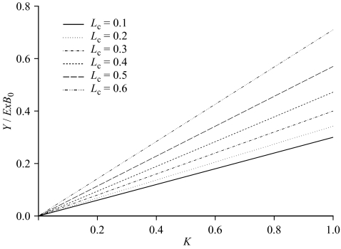
where the parameter a(L_c) is a constant for a given value of the length at first capture L_c). The results are illustrated in figure 1.

Figure 1.

Yield as a proportion of unexploited fishable biomass plotted as a function of K for different values of L_c.

Figure 1 indicates that the potential yield increases with both the size at first capture (L_c) and K, as is well known (e.g. Beverton & Holt 1957). Furthermore, the rate of increase in potential yield with L_c also increases as K increases. However, it is important to remember that situations where both the growth rates and sizes at first capture are high are likely to be relatively uncommon. The exploitable biomass as a proportion of total biomass becomes smaller as italic L_c and K increase. Hence, although in principle potential yields as a proportion of exploited biomass are higher, the absolute yields are smaller and thus unlikely to be commercially attractive unless there are special circumstances.

In figure 1, results have been presented for only values of L_c up to 0.6. In the case of constant recruitment, it is well known that as L_c approaches the eumetric length, L_e, the fishing mortality rate that produces the maximum yield approaches infinity (Beverton & Holt 1957). The eumetric length (relative to L_∞) here is given by (Beddington & Cooke 1983):

$$L_{\text{e}}=\frac{3}{3+M/K},$$ (2.5)

and from the Beverton–Holt invariants M/K = 1.5 and L_e = 0.67, it follows that:

$$L_{\text{e}}=L_{\text{m}}=0.67.$$ (2.6)

A simple equation that captures to a good degree of accuracy the relationship illustrated in figure 1 is as follows:

$$Y/Ex{B}_0=0.2K(1-\ln (0.67-L_{\text{c}})).$$ (2.7)

There is an attraction in using an assumption of constant recruitment as the mathematics are simple and it has been argued that it is a reasonable assumption provided that the SSB is not reduced to low levels. Several authors have suggested that when the level of exploitation is such that SSB is greater then 20% of its unexploited level, then the assumption of constant recruitment is reasonable. However, it is well known that levels of exploitation are often higher than this (Garcia & Grainger 2005) and hence the results for constant recruitment are called into question. We explain the more general case in § 2 b.

(b) Recruitment varying with stock size

Constant recruitment is effectively the limiting case of strong density dependence. A more realistic and conservative approach is to assume that recruitment varies with stock size, with reduced recruitment occurring when the stock size is low.

There is a large literature on stock and recruitment in fish and a variety of models have been proposed (e.g. Quinn & Deriso 1999). In practice, however, it is rarely possible to distinguish between the different models in terms of how well they fit available stock and recruitment data and Kirkwood et al. (1994) chose to use a modified form of the Beverton & Holt (1957) stock–recruitment relationship. They argue that the various stock and recruitment relationships vary between the extreme density dependence of the Ricker (1954) relationship, through constant recruitment to the more conservative form of the Beverton–Holt relationship. This choice seems sensible in the context of developing country fisheries and it has the added advantage that the mathematics are slightly simpler.

According to the Beverton–Holt stock–recruit relationship, the number of recruits first increases rapidly as the SSB increases from zero. As the SSB increases further, the rate of increase in the number of recruits declines, until for very high SSBs, recruitment approaches an asymptote.

The standard formulation of the Beverton–Holt stock–recruit relationship is:

$$R=\frac{\alpha B}{1+\beta B},$$ (2.8)

where R is the number of recruits arising from an SSB of B, and α and β are parameters. In this formulation, α/β is the asymptotic number of recruits, and β is a productivity parameter measuring the rate at which this asymptote is reached.

This formulation is useful when pairs of corresponding estimates of SSB and recruitment are available, as it is a relatively simple matter to estimate the parameters by using regression techniques. Estimates of the parameters α and β are also often reported in the literature when Beverton–Holt relationships have been fitted to stock and recruitment data. In many cases, however, and particularly for developing country fisheries, such data are absent, and it is then very difficult to select realistic values for the parameters.

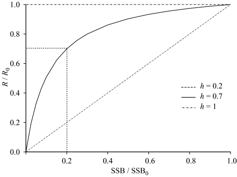
An alternative formulation incorporates a parameter characterizing the ‘steepness‘ of the stock–recruit relationship at low stock sizes. As illustrated in figure 2, the steepness (h) is defined as the recruitment (as a fraction of the recruitment in an unexploited stock) that results when SSB is 20% of its unexploited level, SSB₀ (Mace & Doonan 1988). As h approaches 1, the Beverton–Holt relationship approaches a form in which recruitment is constant; when h is 0.2, recruitment is linearly related to SSB. The great advantage of this formulation is that h is a dimensionless parameter characterizing the shape of the relationship and it is unaffected by the actual size of the stock.

Figure 2.

The characterization of the Beverton–Holt stock–recruit relationship using the steepness parameter, h, for h = 0.2, 0.7 and 1.0.

One further parameter needed for this analysis is the value of L_m. This is the third Beverton–Holt invariant, so that L_m = 0.67.

Kirkwood et al. (1994) illustrated an empirical relationship between potential yield and the natural mortality rate that was almost linear for large areas of parameter space, but varied with L_m, M/K, the degree of density dependence and L_c. The use of the Beverton–Holt invariants significantly simplifies that analysis so that, as in the constant recruitment case, the potential yield as a proportion of unexploited fishable biomass is given (to a close approximation) by the linear relationship:

$$Y/Ex{B}_0=a(L_{\text{c}},h)K,$$ (2.9)

where a(L_c,h) is a constant multiplier of K determined by the length at first capture L_c and the degree of density dependence (steepness) in the stock–recruitment relationship h.

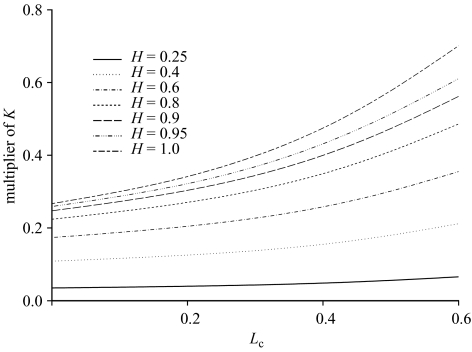
The results are summarized in figure 3.

Figure 3.

Multiplier of K to determine yield as a proportion of unexploited fishable biomass, plotted as a function of L_c for different values of h. The horizontal dotted line is at a level of 0.75, corresponding to the Gulland (1971) formula Y = 0.5MB₀.

As expected, the multiplier of K increases with increased length at first capture and with an increasing degree of density dependence, with constant recruitment being the limiting case as the steepness parameter h approaches 1.

Of particular interest is how quickly yield decreases as the steepness falls below 1, especially for larger values of L_c. Given its definition, it is obvious that reliable estimates of h close to 1 will be available only in cases where the spawning stock size has been reduced to very low levels (i.e. it has been severely overexploited). For many stocks, recruitment appears on average to be constant over the observed range of spawning stock sizes. In such cases, it is often possible to identify a reasonable lower bound for the steepness, but the data would be consistent with any steepness between that and 1. Prudence would therefore indicate that in assessing yield, it would be wise to assume lower values of h (weaker density dependence) until data accumulate to provide evidence to the contrary.

Figure 3 also illustrates clearly the strong bias associated with the use of the Gulland (1971) formula in assessing potential yield. The horizontal line depicting the Gulland relationship lies well above the other lines even for combinations of high density dependence, growth and length at first capture.

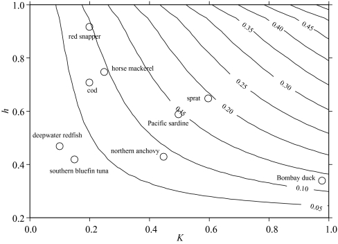
Given the comprehensive collection of stock–recruitment data drawn together by Myers et al. (1995), there is a reasonable literature on estimates of the steepness parameter h. In particular, Myers et al. (1999) summarize estimates of h for a variety of fish species. Combining this information with estimates of the growth parameter K obtainable from FishBase (Froese & Pauly 2004) it is possible to illustrate our results by considering a few typical species. A more exhaustive analysis will be reported elsewhere. The summary results for selected species are shown in figure 4.

Figure 4.

Contours of yield biomass ratios (Y/ExB₀) for different values of K and h. Also shown are estimates of yield biomass ratios for selected fish species, based on estimates for those species of h from Myers et al. (1999) and of K from FishBase (Froese & Pauly 2004). A constant value of L_c of 0.5 has been assumed for each species.

The results presented in figure 4 for individual species are for illustrative purposes only, as there is manifestly substantial uncertainty around the estimates of K and h. Furthermore, we have assumed a constant L_c of 0.5 for each, when in practice the actual lengths at first capture for particular fisheries are likely to be different from this value. Nevertheless, the positioning of the species within the contours illustrates well the general pattern to be expected from the life history of the species concerned.

Estimates of the ratio between potential yield and unexploited fishable biomass for the individual species, and indeed most species, are arguably of historical interest only as almost all have been subject to substantial periods of exploitation. They are nevertheless indicative of the relatively low levels of sustainable yields that are possible and point to the basic reason why so many stocks are over-exploited. In practice, estimates of the original unexploited biomass ExB₀ are rarely available, although for certain species and populations some estimates can be made when long time-series of catch and relative abundance data are available. For new fisheries, particularly where some estimate of biomass has been made, the results can provide useful guidelines for the likely levels of sustainable yields. Recent exploitation of deepwater species, for which growth is known to be very slow would have been arguably less intense if such preliminary results were available. Similarly, the exploitation of newly discovered or relatively lightly exploited stocks can be guided by this analysis to provide an assessment of sustainable yields and hence the level of sustainable fishing capacity.

Of more immediate interest to fishery managers is an idea of whether the current level of exploitation of a stock is sustainable. In § 3, we explore this issue using similar techniques to those for the estimation of sustainable yield, but this time we focus on the fishing mortality rate that produces the maximum sustainable yield. If this is known and the current fishing mortality rate can be estimated, then the sustainability of current levels of fishing can be assessed.

3. Stock status

In addition to comparing recent and current catches to estimates of potential yield, the status of a fished stock can also be assessed by comparing an estimate of the current fishing mortality rate with an estimate of the fishing mortality rate that produces the maximum yield, F_max.

Both Beverton & Holt (1957) and Gulland (1971) observed that in many situations, F_max was related to and often close to the level of the annual instantaneous natural mortality rate, M. Other authors have also made similar observations but, to our knowledge, no studies have been carried out to elucidate this relationship. The above analysis would appear to have two implications. First, whatever relationship exists between F_max and M, it is likely to hold only for a particular L_c. Second, it is likely that F_max (for particular L_c) may be a simple fraction of the growth parameter K.

(a) Constant recruitment

Confirming that suggestion, using the techniques of Kirkwood et al. (1994) and the Beverton–Holt invariants, it can be shown that for L_c < L_m, in the case of constant recruitment a linear relationship holds between F_max and K. Specifically:

$$F_{\max }=a(L_{\text{c}})K$$ (3.1)

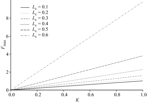
where the coefficient a(L_c) varies with the length at first capture. The results are illustrated in figure 5.

Figure 5.

F_max as a function of K for different values of L_c, when recruitment is assumed constant.

As with the comparable relationship between yield biomass ratios and K discussed earlier, F_max increases with increasing K and increasing L_c. Now, however, the relationship with L_c is much more non-linear for larger L_c, reflecting the fact that F_max approaches infinity as L_c approaches 0.67.

Because of the extreme density dependence implicit in an assumption of constant recruitment, the F_max predicted in this case is almost certainly an upwardly biased estimate of the true F_max. It follows, therefore, that if the current fishing mortality rate is estimated to be close to or above this F_max, then it is likely that the stock is being overexploited.

A simple equation that captures to a good degree of accuracy the relationship illustrated in figure 5 for L_c < L_m is as follows:

$$F_{\max }=\frac{0.6K}{0.67-L_{\text{c}}}.$$ (3.2)

(b) Recruitment varying with stock size

If, as before with potential yield, we make the more prudent and realistic assumption that recruitment varies with SSB according to a Beverton–Holt stock–recruitment relationship, then to a close approximation F_max is linearly related to K. In this case, however, the equation is:

$$F_{\max }=a(L_{\text{c}},h)K,$$ (3.3)

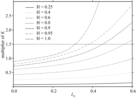
where a(L_c,h) is a constant depending on the values of L_c and the degree of density dependence h. The results in terms of values of the multiplier of K are summarized in figure 6.

Figure 6.

Multiplier of K to determine F_max, plotted as a function of L_c for different values of h. The horizontal dotted line corresponds to a K multiplier of 1.5, when F_max = M2.

The results shown in figure 6 indicate the very strong influence that the steepness h has on F_max. In practice, h is a relatively difficult parameter to estimate reliably, requiring at least a substantial time series of stock and recruitment data corresponding to a wide range of spawning stock sizes. Because of this, it is not surprising that the estimates reported in Myers et al. (1999) are predominantly for temperate species subject to substantial fisheries. For developing country fisheries, it may therefore be rather difficult to obtain reliable direct estimates of h, though it may be possible to infer possible ranges from published estimates for similar species elsewhere. In such circumstances, a relatively low choice of h would appear to be prudent.

The horizontal dotted line in figure 6 corresponds to a multiplier of K of 1.5, which is equivalent to F_max being equal to M. It will be recalled that a number of authors since Beverton & Holt (1957) have observed that, for certain species, F_max was approximately equal to M. While this is true for certain combinations of K and h, it seems likely that the relationship claimed is an artefact of the choice of species examined, as the region close to a multiplier of K of 1.5 is only a very small part of feasible parameter space.

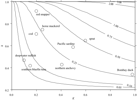
The results obtained from the set of selected species used in § 3a are presented in figure 7.

Figure 7.

Contours of F_max for different values of K and h. Also shown are estimates of F_max for selected fish species, based on estimates for those species of h from Myers et al. (1999) and of K from FishBase (Froese & Pauly 2004). A constant value for L_c of 0.5 has been assumed for each species.

As noted before, the results presented for individual species are for illustrative purposes only, given the uncertainties associated with them. Again, however, the positioning of the species within the contours illustrates well the general pattern to be expected from their life histories.

4. Caveats

To produce the results presented here, it has been necessary to make a number of simplifying assumptions. The first is that all fishes with lengths greater than L_c are equally vulnerable to capture. Manifestly, real fisheries do not operate in this manner; typically, they are prosecuted using a variety of fishing gears that have different selection patterns with size (and age). Usually, for each gear it is possible to identify an average length at first capture. If one gear dominates catches, then setting L_c equal to the average length at first capture for that gear should be sufficient. If there are many gears catching a wide range of sizes, and setting L_c equal to the smallest average length at first capture would be prudent. The hardest case is when there are two substantial gears catching over quite different size ranges (e.g. purse seine and long-line fisheries for tunas), but even here, selecting an L_c based on the smaller average length at first capture seems the most sensible course of action.

The Beverton–Holt invariants and their various derivations produce an estimate of the relationship between M and K with growth assuming that the natural mortality rate is constant over the relevant part of the lifespan. However, in a number of species, age- or length-specific patterns of natural mortality have been observed. Kirkwood et al. (1994) were able to show that in this case, a simple Heincke estimator (Heincke 1913) will give a reasonable estimate of the average natural mortality rate that relates well to the natural mortality rate involved in the derivation of the invariants.

By ignoring stochastic effects, the analysis presented here fails to account for a ubiquitous characteristic of fish stocks, namely that they fluctuate constantly. Such fluctuations are difficult to quantify and in most circumstances they are impossible to predict. However, again Kirkwood et al. (1994) showed that their deterministic analysis still provides a reasonable guide to the average behaviour of stocks that are exploited in fluctuating environments.

In some species, there is evidence that density dependence operates on both growth and mortality of post-recruits, as well as via the stock recruitment process (e.g. Beverton & Holt 1957; Lorenzen & Enberg 2002). In this situation, the analysis is substantially more complicated, but the estimate of potential yield at F_max obtained on the assumption that density dependence only occurs via the stock–recruitment relationship is likely to be conservative (Kirkwood et al. 1994).

5. Assessing stock status

The results above have a useful practical implication for the assessment of the status of fisheries where data are sparse. Given an estimate of growth parameters for the species concerned, an estimate of F_max can be obtained simply by application of equation (3.3). For data-rich fisheries, there are many methods available for estimating the current F that are routinely used in annual stock assessments, but it is often not possible to use these methods when data are sparse. Fortunately, however, several other (albeit rather imprecise) methods for estimating the current total mortality rate (F + M) that rely simply on availability of catch length frequency samples and estimates of growth parameters have been incorporated into stock assessment software packages commonly used in developing countries (e.g. FiSAT; Gayanilo & Pauly 1997). It is then a simple matter to estimate F by applying the Beverton–Holt invariant M = 1.5K. Alternatively, if an estimate of current biomass is available, for example from a survey, then a simple approximate estimate of F is available from the ratio of current catch to current biomass.

If the current estimate of F is substantially higher than F_max, then the stock is clearly being overexploited and action may be needed to avert a stock collapse. If it is close to F_max, then any increase in fishing effort should be discouraged. In the situation where the estimate of F is well below F_max, then some simple guidelines for expansion of the fishery may be used. Increasing catch levels by increasing effort can be permitted as long as the new F is still below F_max. Clearly, prudence will require that it is a reasonable level below.

6. Concluding remarks

In this paper, we have developed simple relationships that can be used to estimate potential yield and the maximum sustainable fishing mortality rate given information on the growth curve and size at which fishing starts. In both cases, this information can be obtained relatively easily from standard sampling procedures well within the capability of developing country fisheries institutions. The level of potential yield and the corresponding fishing mortality rate depend also on the steepness (the degree of density dependence) in the stock–recruit relationship, which is much less easy to estimate. However, the results in this paper still allow estimates to be calculated for a reasonable range of possible values of steepness, thereby allowing prudent management decisions to be made when only sparse data are available.

Glossary

SSB

spawning stock biomass

References

- Beddington J.R., Cooke J.G. On the potential yield of fish stocks. 1983. FAO Fisheries Technical Paper 242. [Google Scholar]
- Beverton R.J.H., Holt S.J. On the dynamics of exploited fish populations. MAFF Fish. Invest. Lond. Ser. 2. 1957;19:1–533. [Google Scholar]
- Beverton R.J.H., Holt S.J. A review of the lifespans and mortality rates of fish in nature and the relationship to growth and other physiological characteristics. Ciba Found. Colloq. Age. 1959;5:142–177. [Google Scholar]
- Branch T.A., Kirkwood G.P., Nicholson S.A., Zara S.J. YIELD version 1.0. MRAG Ltd; London: 2001. [Google Scholar]
- Charnov E.L. Life history invariants. Oxford University Press; New York: 1993. [Google Scholar]
- Charnov E.L., Berrigan D. Dimensionless numbers and life history evolution: age of maturity versus the adult lifespan. Evol. Ecol. 1990;4:273–275. [Google Scholar]
- Clark W. Groundfish exploitation rates based on life history parameters. Survival. Can. J. Fish. Aquat. Sci. 1991;48:734–750. [Google Scholar]
- Froese R., Binohlan C. Empirical relationships to estimate asymptotic length, length at first maturity and length at maximum yield per recruit in fishes, with a simple method to evaluate length frequency data. J. Fish Biol. 2000;56:758–773. [Google Scholar]
- Froese R., Pauly D., editors. 2004. FishBase. World Wide Web electronic publication. See www.fishbase.org, version (06/2004) [Google Scholar]
- Garcia S.M., Grainger R.J.R. Gloom and doom? The future of marine capture fisheries. Phil. Trans. R. Soc. B. 2005;360:21–46. doi: 10.1098/rstb.2004.1580. doi:10.1098/rstb.2004.1580 (In this issue.) [DOI] [PMC free article] [PubMed] [Google Scholar]
- Gayanilo F.C. Jr, Pauly D., editors. FAO computerized information series (fisheries), no. 8. FAO; Rome: 1997. The FAO-ICLARM stock assessment tools (FiSAT) reference manual. [Google Scholar]
- Gulland J.A. The fish resources of the ocean. Fishing News Books; West Byfleet, UK: 1971. [Google Scholar]
- Heincke F. Investigations on the plaice. General report 1. The plaice fishery and protective measures. Preliminary brief summary of the most important points of the report. Rapp. Pv Reun. Cons. int. Explor. Mer. 1913;16:1–67. [Google Scholar]
- Jensen A.L. Beverton and Holt life history invariants result from optimal trade-off of reproduction and survival. Can. J. Fish. Aquat. Sci. 1996;53:820–822. [Google Scholar]
- Kirkwood G.P., Beddington J.R., Rossouw J.R. Harvesting species of different lifespans. In: Edwards P.J., May R., Webb N.R., editors. Large-scale ecology and conservation biology. Blackwell Scientific; Oxford: 1994. pp. 199–227. [Google Scholar]
- Lorenzen K., Enberg K. Proc. R. Soc. B. 2002;269:49–54. doi: 10.1098/rspb.2001.1853. doi:10.1098/rspb.2001.1853 [DOI] [PMC free article] [PubMed] [Google Scholar]
- Mace P.M., Doonan I.J. A generalized bioeconomic simulation model. NZ fisheries assessment research document no 88/4. 1988 [Google Scholar]
- Mangel M. Evol. Ecol. 1996;10:249–263. [Google Scholar]
- Myers R.A., Bridson J., Barrowman N.J. Summary of worldwide spawner and recruitment data. 1995. Canadian Technical Report Fisheries and Aquatic Science 2024. [Google Scholar]
- Myers R.A., Bowen K.G., Barrowman N.J. Can. J. Fish. Aquat. Sci. 1999;56:2404–2419. [Google Scholar]
- Pauly D. J. Conserv. Int. Explor. Mer. 1980;11:559–623. [Google Scholar]
- Quinn II T.J., Deriso R.B. Oxford University Press; 1999. [Google Scholar]
- Ricker W.E. J. Fish. Res. Bd. Can. 1954;30:1965–1976. [Google Scholar]
- Roff D.A. Can. J. Fish. Aquat. Sci. 1984;41:989–1000. [Google Scholar]
- von Bertalanffy L. Hum. Biol. 1938;10:181–213. [Google Scholar]