Estimation of Pharmacokinetic Parameters Based on the Patient-Adjusted Population Data

Abstract

Population pharmacokinetic data, adjusted for patient characteristics, are recommended for the design of initial dosage regimens of some therapeutically monitored drugs in patients for whom patient-specific data are not available. However, despite widespread use by clinicians such as pharmacists, a clear understanding of the principles of population pharmacokinetics, including data collection and analysis and its limitations, is often lacking. This article describes the 2 main methods of obtaining population kinetic data, namely the two-stage method and nonlinear mixed effect model, and their applications to the pharmacokinetic-based design of dosage regimens. Additionally, some numerical examples are provided to assist the reader in understanding the material. The author uses these tools in a pharmacokinetics course taught to PharmD students.

INTRODUCTION

Nomograms or equations, which describe the relationships between patient characteristics and pharmacokinetic parameters in a population, are often used to estimate the initial pharmacokinetic parameters for drug dosing in individual patients for whom patient-specific parameters are not known.^1-3 Examples of patient characteristics are age, weight, gender, disease state(s), interacting drug(s), or environmental factor(s) (eg, smoking and food). For instance, population data indicate that there is a significant relationship between the clearance (CL) of digoxin and the creatinine clearance (a measure of how well the kidneys function).^4,5 As creatinine clearance (CL_CR) decreases, so does the clearance of digoxin. One can actually use the reported population-based relationship for digoxin to estimate a clearance value in an individual patient based on his/her creatinine clearance.

Population-based nomograms or equations have been recommended for initial dosing of most drugs currently subjected to therapeutic drug monitoring, including aminoglycosides,^2,6-11 digoxin,^4,12-15 and theophylline,^16-18 among others. Although pharmacy students are exposed to these equations/nomograms during their didactic education and, sometimes, use them in their clinical rotations, they may not have a clear understanding of the origins and limitations of these data. Therefore, this instructor devotes a 75-minute session of the Clinical Pharmacokinetics course to the pharmacokinetic analysis of population data and its application to the estimation of initial pharmacokinetic parameters in individual patients. This article describes the learning tools that the author uses for this session.

The specific learning objectives of the session are for students to accomplish the following:

1. Devise a general approach for individualization of dosage regimen in a patient.

2. Differentiate between the 2 main methods (Two-Stage and Mixed Effect Model) used for obtaining population pharmacokinetic data.

3. Develop regression relationships between the population pharmacokinetic parameters and patient characteristics that are continuous in nature, such as age, weight, and creatinine clearance.

4. Categorize patients into subpopulations based on discrete patient characteristics, such as gender, presence or absence of disease states, and/or smoking status, and estimate subpopulation pharmacokinetic parameters.

5. Evaluate the clinical and statistical significance of the population-based regression or categorization relationships.

6. Estimate the individual patient pharmacokinetic parameters from the population relationships.

INSTRUCTIONAL METHODS

The details of the educational environment¹⁹ and the format²⁰ of the course have already been published. In the following sections, instructional tools, such as reading handouts, practice problems, and assessment tools used in this session are discussed. The reading assignment, described below, is provided online to students and must be completed before attending the class session for the discussion of the topic. Additionally, other readings from a suggested textbook¹ and some articles^21-23 serve as optional reading assignments.

General Approach for Individualization of Dosage Regimens

The individualization of dosage regimen usually involves 3 steps.

Design of initial dosage regimen

When a patient is to be treated with a drug for the first time, or whenever the pharmacokinetic parameters of the drug in the individual patient are not known, one may recommend a dosage regimen (dose and dosage interval) based on either of the following 2 methods:

1. To recommend a general dosage regimen for all the patients based on the recommendations of the manufacturer. In most cases, this method may take into account only the bodyweight or surface area of the patient for individualization.

2. To use the so-called adjusted population pharmacokinetic parameters, which are based on the population values adjusted for the patient characteristics, to design a dosage regimen based on pharmacokinetic principles.

Estimation of patient-specific pharmacokinetic parameters

Blood samples should be taken at appropriate times after the administration of the initial dosage regimen to determine the patient-specific pharmacokinetic parameters, which may be different from those estimated based on the adjusted population values.

Adjustment of dosage regimen

If the measured blood concentrations are in agreement with the concentrations predicted from the adjusted population values, no dosage adjustment is necessary. However, if the measured plasma concentrations are not appropriate, the patient-specific pharmacokinetic parameters should be used to determine a new dosage regimen for the patient. In that case, subsequent blood samples should be taken to verify the achievement of the desired concentrations. The estimation of patient-specific parameters and dosage regimen adjustment should be repeated until the desired plasma concentrations are achieved and maintained.

Estimation of Population Pharmacokinetic Data

Traditional (two-stage) method

One of the main methods for obtaining population pharmacokinetic data is the traditional (or two-stage) method. In the first stage of this method, the drug is administered to a group of patients and a relatively large number of samples is obtained from each patient in order to conduct a full pharmacokinetic analysis to determine the pharmacokinetic parameters of the drug in each patient. In the second stage, the average and standard deviation for each pharmacokinetic parameter are estimated using the individual values. Additionally, the relationships between the pharmacokinetic parameters and patient characteristics (such as age, weight, gender, and degree of renal function), presence or absence of interacting drugs, or environmental factors are determined by categorization and/or regression analysis as explained below.

Categorization is done when the patient population can be divided into subpopulations (categories). For example, smoker and nonsmoker patients may be separated and the mean and standard deviation of the kinetic parameters estimated separately in each subpopulation. Statistical tests (such as t test) may then be used to determine whether the difference between the 2 subgroups in each pharmacokinetic parameter is true or due to random variability. For example, theophylline clearance in heavy smokers is significantly (~60%) higher than the values in nonsmokers. However, the mean value for the combined population of smokers and nonsmokers is somewhere in between the values in the 2 populations.^1,24 Other examples of categorization could be females vs. males and presence or absence of a disease state (eg, cirrhosis or congestive heart failure) or an interacting drug (such as cimetidine or rifampin).

Regression is done when a relationship between 2 continuous variables can be established, as opposed to categorization when a condition exits or does not exist. A clinically important example of the use of regression in population analysis is the relationship between the patient creatinine clearance and the clearance of drugs that are partially or totally eliminated by renal clearance. The total clearance of a drug is a summation of renal clearance (CL_R) and nonrenal clearances (CL_NR):

Additionally, clearance of drugs is proportional to the creatinine clearance of the patient with a proportionality constant of α:

Therefore, the relationship between the total clearance and creatinine clearance can be written as follows:

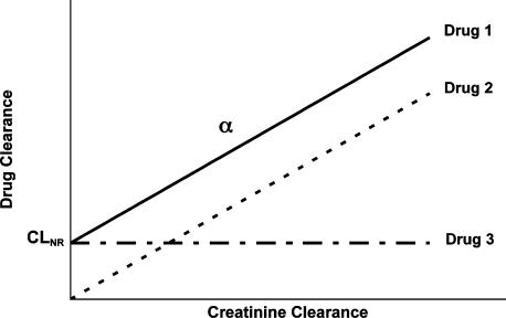
This equation indicates that when the clearance of a drug in a patient population with different degrees of renal function (different values of creatinine clearance) is plotted against creatinine clearance, a linear relationship is expected with a slope of α and an intercept of nonrenal clearance. In theory, 3 different types of relationships may exist depending on the characteristics of the drug (Figure 1). Drug 1 is eliminated by both renal and nonrenal pathways. For this drug, both the y-intercept (nonrenal clearance) and the slope (α) are significantly greater than zero. Drug 2 is eliminated only via the renal pathway; the y-intercept (nonrenal clearance) is zero for this drug. Lastly, drug 3 is not eliminated by the renal pathway at all (the slope is zero). Therefore, the clearance of drug 3 is not affected by the magnitude of creatinine clearance.

Figure 1.

Possible relationships between the drug clearance and the patient creatinine clearance for three hypothetical drugs.

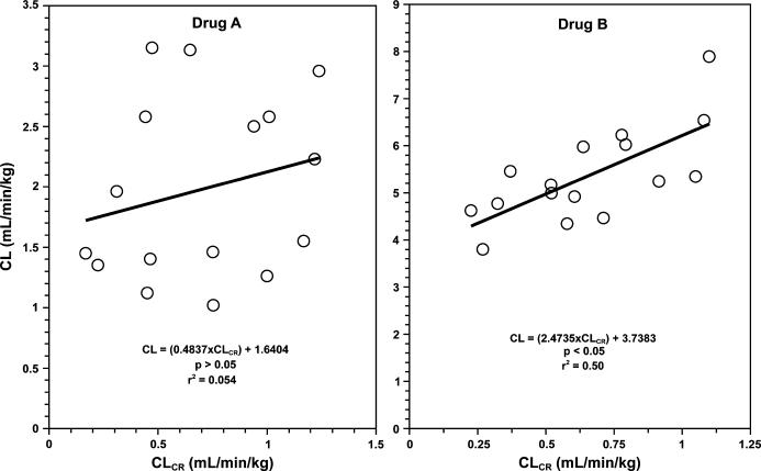
In practice, these relationships (Figure 1) are not perfect in that there may be a significant degree of scatter around the lines. This is mainly due to interindividual variability in the values of intercept (nonrenal clearance) and slope (α) among the patient population, in addition to observation variability that is due to measurement error. Therefore, the relationships need to be carefully examined in order to assure that the relationship between the total clearance and creatinine clearance is clinically and statistically significant and not due to random error or variability. This may be done through regression analysis, which reveals the significance of regression of y against x (p value) and the degree by which the changes in y may be explained by changes in x (r² or coefficient of determination). For example, consider the data in Figure 2 for 2 hypothetical drugs (A and B), where one cannot say with certainty whether there is a significant relationship between the 2 parameters by just plotting the data and observing the trend. However, a regression analysis of the relationship for drug A indicates a p value of >0.05, suggesting that the apparent relationship between the 2 parameters (Figure 2, drug A) is not statistically significant. Additionally, the very low r² value of 0.054, implying that only 5% of the variability in clearance may be explained by changes in creatinine clearance, shows that even if this relationship were statistically significant, it would be of no clinical relevance. Therefore, one may conclude that the degree of renal function would not significantly affect the clearance of this drug. On the other hand, a statistical analysis of the data for drug B shows a p value of <0.05 for the regression, indicating that the clearance of the drug is significantly dependent on the creatinine clearance of the patient. Furthermore, the r² value of 0.50 suggests that ~50% of the variability in the clearance value in this population may be explained by differences in the creatinine clearance of the patients. In this case, the y-intercept (nonrenal clearance) is 3.74 mL/min/kg and the slope (α) is 2.47. Therefore, the following population relationship may be constructed for this drug:

Figure 2.

The non-significant (Drug A) and significant (Drug B) relationships between the drug clearance (CL) and the patient creatinine clearance (CL_CR) in a small population of sixteen patients for two hypothetical drugs. Drug A: CL = (0.484 × CL_CR) +1.64, p > 0.05, r² = 0.054; Drug B: CL = (2.47 × CL_CR) +3.74, p < 0.05, r² = 0.50.

This means that equation 4 may be used to estimate the clearance of drug B in a new patient with a known value of creatinine clearance. For example, clearance in a 66-kg patient with a creatinine clearance of 35 mL/min (0.53 mL/min/kg) would be 5.05 mL/min/kg or 333 mL/min:

Similar relationships have been reported for some drugs that are therapeutically monitored. For example, the following relationship was reported⁵ for digoxin in 10 subjects with different degrees of renal function:

The regression analysis is not only for the relationship between clearance and creatinine clearance. There may be significant relationships between other pharmacokinetic parameters in addition to clearance, such as volume of distribution (V) or elimination rate constant (k), and other continuous patient characteristics in addition to creatinine clearance, such as age, body weight (total, lean, ideal, or adjusted), or serum creatinine concentration. For example, the following relationship was reported⁸ between the k of aminoglycosides and the patient creatinine clearance:

The theoretical basis of equation (6) is similar to that for equation (1) in that the overall elimination rate constant (k) is the summation of renal (0.0024 CL_CR) and nonrenal (0.01) rate constants. As equation (6) clearly shows, the units of x and y in these regression relationships are only related to the units of data used for the regression analysis, and hence do not have to cancel out. This is especially true when the y and x axes are totally different parameters, such as regression of clearance (unit of volume per time) versus age (unit of time) or regression of volume of distribution (unit of volume) versus body weight (unit of mass). For example, Bauer et al¹⁰ demonstrated the following relationship between the volume of distribution of amikacin and total (TBW) and ideal (IBW) body weights in 7 morbidly obese patients:

This empirical relationship suggests that amikacin, in addition to its distribution into the extracellular volume of IBW, would also distribute into 10% of the fat weight (total body weight-ideal body weight) in obese patients.

The advantages of the two-stage method are its simplicity, the use of standard data analysis, individual estimates of pharmacokinetic parameters, and controlled experimental conditions allowing unbiased definition of relationships between pharmacokinetic parameters and the factor of interest.²⁵ However, the method also has limitations such as its high cost, necessitating inclusion of only a small number of patients, and ethical problems of extensively studying patients who may not directly benefit from the study. Therefore, caution should be exercised when using reported population pharmacokinetic relationships based on this method because most of these data have been obtained in a small number of tightly controlled patients, making extrapolations to other patient populations extremely risky.

Nonlinear mixed effects model

A second method for obtaining population data is based on a statistical method called the nonlinear mixed effects model. In this method, instead of obtaining a large number of samples in each individual (two-stage method), a limited number of samples (1-6) is obtained from each patient during routine clinical monitoring,⁴ rendering estimation of pharmacokinetic parameters in individual patients difficult, if not impossible. Instead, the data from all the patients is put together and the average and variability of the pharmacokinetic parameters are estimated for the whole population rather than in each individual patient. The results of this method are fixed effects (such as the intercept and slope of equation 1 for the average or typical patient), random effects (the variability in the pharmacokinetic parameter value in an individual versus the typical patient or inter-individual variability), and observation or error terms (such as measurement error). One of the main advantages of this method is that any concentration-time data obtained during the development phase of the drug or routine clinical monitoring of the patient can be incorporated into a database and used for the population kinetic analysis. For example, the samples do not have to be obtained at the same time in different patients. Additionally, the dosage regimens may be different for different patients. This method, however, requires complex computer programs, such as NONMEM (GloboMax, Ellicott City, MD) to handle the calculations and can produce meaningful results only if the number of patients studied is large.²⁵ This method was used by Sheiner et al⁴ for determining the population clearance and volume of distribution of digoxin in 141 patients in relation to their creatinine clearance and the severity of congestive heart failure (CHF), resulting in the following relationships:

The above relationships for digoxin indicate that renal dysfunction would affect both the clearance and volume of distribution of the drug. As expected, a reduction in creatinine clearance results in a reduction in the clearance of digoxin (equations 8 and 9). However, in the subpopulation with more severe congestive heart failure, the non-renal clearance of the drug (0.020 L/h/kg) is substantially lower than that in the subgroup with less severe congestive heart failure (0.0489 L/h/kg). As for volume of distribution, equation 10 indicates that renal dysfunction (reduction in creatinine clearance) also would result in a reduction in the volume of distribution of digoxin. This is because in renal dysfunction, the tissue binding of digoxin may be reduced, resulting in shifting the drug to plasma.¹³

Other methods

A number of other methods have also been proposed and used for analysis of population pharmacokinetic data.^22,26 Most of these methods are different variations of the 2 methods explained above and their discussion is out of the scope of this introductory session.

Application of Population Data

Once the relationships between the pharmacokinetic parameters and patient characteristics are developed using the two-stage or the mixed-effects model, they may be used to estimate the approximate values of pharmacokinetic parameters in an individual patient. Additionally, the population data, along with plasma concentration data, may be used in later stages of dosage regimen individualization for estimation of patient-specific pharmacokinetic parameters using Bayesian analysis.

An Example of the Two-Stage Method

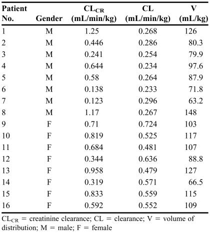
The clearance and volume of distribution of a drug, estimated in 16 patients (males and females) with varying degrees of renal function during stage 1 of the two-stage method, are reported in Table 1. You are asked to estimate the mean and standard deviation of the kinetic parameters (clearance and volume of distribution) and develop appropriate population relationships between these pharmacokinetic parameters and patient characteristics (stage 2). Furthermore, using the data developed in stage 2, determine the pharmacokinetic parameters in the 2 patients described in Table 2 who will be treated with the drug for the first time.

TABLE 1.

Patient Characteristics and Pharmacokinetic Parameters of a Drug Obtained During Stage One of the Two-Stage Method After Intravenous Administration

CL_CR = creatinine clearance; CL = clearance; V = volume of distribution; M = male; F = female

TABLE 2.

Patient Characteristics Used to Determine Pharmacokinetic Parameters When Data Are Not Available

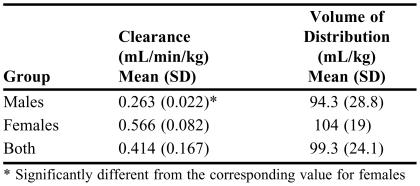
First, one may calculate the average and standard deviation values of the pharmacokinetic parameters in the whole population and also after categorization of the data into the 2 possible subpopulations of male and female patients (Table 3). To determine whether there are significant differences among subpopulations, statistical tests such as analysis of variance (ANOVA; when more than 2 subpopulations are examined) or unpaired t test (when 2 groups are compared) may be used to compare the mean values of the kinetic parameters in the subpopulations. In this case, the mean clearance in female patients (0.566 mL/min/kg) is more than twofold higher than that in male patients (0.263 mL/min/kg) (Table 3). An unpaired, 2-tailed t test comparison of the means reveals a p value of <0.0000001, indicating that the difference in clearance between male and female patients is statistically significant. On the other hand, the volume of distribution in male patients (94.3 mL/kg) is not significantly different (p = 0.433) than that in female patients (104 mL/kg).

TABLE 3.

Pharmacokinetic Parameters

* Significantly different from the corresponding value for females

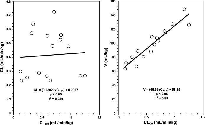
One could also examine whether there is any significant regression relationships between the pharmacokinetic parameters (clearance or volume of distribution) and continuous population characteristics (creatinine clearance in this case). The regression analysis of clearance against creatinine clearance (Figure 3, left panel) reveals an intercept of 0.396 mL/min/kg and a slope of 0.0302. However, the p value of slope is 0.82 and r² is 0.030, indicating that the relationship between the 2 is not significant. On the other hand, the relationship between volume of distribution and creatinine clearance (Figure 3, right panel) results in an intercept of 58.2 mL/kg and a significant slope of 66.6 (p < 0.0000001), indicating that the volume of distribution of the drug changes in renal dysfunction.

Figure 3.

The relationships between the drug clearance (CL, left panel) or volume of distribution (V, right panel) and the patient creatinine clearance (CL_CR) in a small population of sixteen patients for a hypothetical drug. Clearance: CL = (0.0302 × CL_CR) +0.396, p > 0.05, r² = 0.030; Volume of distribution: V = (66.6 × CL_CR) +58.2, p < 0.05, r² = 0.88.

Therefore, the following relationship can be established for volume of distribution:

Overall, the regression (Figure 3) and categorization (Table 3) data obtained above may be used to adjust the population pharmacokinetic data for individual patients. This is demonstrated for the 2 patients described in Table 2.

Patient A

The clearance of the drug is not dependent on creatinine clearance (Figure 3, left panel). However, the clearance in male patients is different than that in female patients (Table 3). Because this patient is male, a clearance of 0.263 mL/min/kg or 16.8 (0.263 × 64) mL/min should be used. As for volume of distribution, it is not dependent on the gender (Table 3). However, the relationship developed above (equation 11) should be used to estimate volume of distribution in this patient:

Patient B

Because this patient is female, a clearance of 0.566 mL/min/kg or 40.8 (0.566 × 72) mL/min should be used. Additionally, the estimated volume of distribution in this patient is 5.56 L:

Pharmacokinetic-Based Design of Dosage Regimens

Once the adjusted population pharmacokinetic parameters are estimated in individual patients, dosage regimens (dose and dosage interval for multiple dosing or infusion rate for constant intravenous infusion) may be designed based on the pharmacokinetic principles. This topic, which is based on both pharmacokinetic parameters and the desired maximum and minimum blood concentrations, is covered in a separate session.²⁷ Additionally, the subsequent processes in individualization of dosage regimens, such as estimation of patient-specific pharmacokinetic parameters through least squares regression or Bayesian analysis, are covered in another session in this course.

Practice Problems and Assessment Tools for the Session

In addition to the reading handout discussed above, the students are provided with a practice problem ahead of the scheduled session. The practice problem is similar to the example discussed above. However, in addition to the above calculations, students are required to use the estimates of volume of distribution and clearance in the patient to calculate the loading and maintenance doses, respectively, when the target drug concentration and dosing interval are provided. Students are expected to work on the problem before attending the class, consulting the reading note. After a brief introduction of the topic by the instructor, the class time is mostly devoted to discussion of the solution to the practice problem by both the students and the instructor.

During the last 10 minutes of the 75-minute session, students take an online quiz²⁸ consisting of questions related to the topic of population pharmacokinetics covered during the session. Finally, students are required to submit an individualized, online assignment²⁹ by the end of the day the session is held. For data analysis, students use Microsoft Excel, which provides descriptive statistics (such as mean and standard deviation), t test, and regression analysis. Additional written step-by-step instructions are also provided to students for using the Excel program in the required statistical analyses.

OUTCOMES

After the completion of this session and take-home assignment, the students should achieve the following outcomes:

1. Understand the overall process for pharmacokinetic-based design and modification of dosage regimens in individual patients.

2. Develop relationships (regression or categorization) to relate the reported kinetic parameters of drugs to the characteristics of the population (eg, weight, age, gender, creatinine clearance) in which the data were obtained.

3. Adjust the population kinetic data for the individual patient who has not been treated with the drug before and/or for whom the patient-specific pharmacokinetic parameters are not yet available.

SUMMARY

The learning tools used in a Clinical Pharmacokinetics course for the topic of population pharmacokinetics, which is taught to PharmD students at Texas Tech School of Pharmacy, are described here. These tools include a reading handout containing numerical examples, a practice problem as the basis of class discussion, an in-class quiz at the end of the session, and a take-home assignment. It is the instructor's belief that these tools facilitate the learning of this relatively difficult topic and make students appreciate the advantages and limitations of the use of population pharmacokinetic data in the design of dosage regimens.

REFERENCES

- 1.Rodman J, D'Argenio D, Peck C. Analysis of pharmacokinetic data for individualizing drug dosage regimens. In: Burton M, Shaw L, Schentag JJ, Evans WE, editors. Applied Pharmacokinetics & Pharmacodynamics: Principles of Therapeutic Drug Monitoring. 4th ed. Philadelphia, Pa: Lippincott Williams & Wilkins; 2006. pp. 40–59. [Google Scholar]
- 2.Hull JH, Sarubbi FA., Jr Gentamicin serum concentrations: pharmacokinetic predictions. Ann Intern Med. 1976;85:183–9. doi: 10.7326/0003-4819-85-2-183. [DOI] [PubMed] [Google Scholar]
- 3.Winter ME. Basic Clinical Pharmacokinetics. 4th ed. Philadelphia, Pa: Lippincott Williams & Wilkins; 2004. pp. 129–476. [Google Scholar]
- 4.Sheiner LB, Rosenberg B, Marathe VV. Estimation of population characteristics of pharmacokinetic parameters from routine clinical data. J Pharmacokinet Biopharm. 1977;5:445–79. doi: 10.1007/BF01061728. [DOI] [PubMed] [Google Scholar]
- 5.Koup JR, Jusko WJ, Elwood CM, Kohli RK. Digoxin pharmacokinetics: role of renal failure in dosage regimen design. Clin Pharmacol Ther. 1975;18:9–21. doi: 10.1002/cpt19751819. [DOI] [PubMed] [Google Scholar]
- 6.DiPiro J, Spruill W, Blouin R, Pruemer J, editors. Concepts in Clinical Pharmacokinetics. 3rd ed. Bethesda, Md: American Society of Health-System Pharmacists; 2002. Aminoglycosides, Lesson 12; pp. 189–209. [Google Scholar]
- 7.Beringer P, Winter ME. Aminoglycoside antibiotics. In: Winter ME, editor. Basic Clinical Pharmacokinetics. 4th ed. Philadelphia, Pa: Lippincott Williams & Wilkins; 2004. pp. 130–71. [Google Scholar]
- 8.Sarubbi FA, Jr, Hull JH. Amikacin serum concentrations: prediction of levels and dosage guidelines. Ann Intern Med. 1978;89:612–8. doi: 10.7326/0003-4819-89-5-612. [DOI] [PubMed] [Google Scholar]
- 9.Erdman SM, Rodvold KA, Pryka RD. An updated comparison of drug dosing methods. Part III: Aminoglycoside antibiotics. Clin Pharmacokinet. 1991;20:374–88. doi: 10.2165/00003088-199120050-00003. [DOI] [PubMed] [Google Scholar]
- 10.Bauer LA, Blouin RA, Griffen WO, Jr., Record KE, Bell RM. Amikacin pharmacokinetics in morbidly obese patients. Am J Hosp Pharm. 1980;37:519–22. [PubMed] [Google Scholar]
- 11.Chan RA, Benner EJ, Hoeprich PD. Gentamicin therapy in renal failure: a nomogram for dosage. Ann Intern Med. 1972;76:773–8. doi: 10.7326/0003-4819-76-5-773. [DOI] [PubMed] [Google Scholar]
- 12.DiPiro J, Spruill W, Blouin R, Pruemer J, editors. Concepts in Clinical Pharmacokinetics. 3rd ed. Bethesda, Md: American Society of Health-System Pharmacists; 2002. Phenytoin and digoxin, Lesson 15; pp. 255–71. [Google Scholar]
- 13.Winter ME. Digoxin. In: Winter ME, editor. Basic Clinical Pharmacokinetics. 4th ed. Philadelphia, Pa: Lippincott Williams & Wilkins; 2004. pp. 183–221. [Google Scholar]
- 14.Mutnick A. Digoxin. In: Schumacher G, editor. Therapeutic Drug Monitoring. Norwalk, Ct: Appleton & Lange; 1995. pp. 469–91. [Google Scholar]
- 15.Dettli L, Ohnhaus EE, Spring P. Digoxin dosage in patients with impaired kidney function. Br J Pharmacol. 1972;44:373P. [PMC free article] [PubMed] [Google Scholar]
- 16.Powell JR, Vozeh S, Hopewell P, Costello J, Sheiner LB, Riegelman S. Theophylline disposition in acutely ill hospitalized patients: the effect of smoking, heart failure, severe airway obstruction, and pneumonia. Am Rev Respir Dis. 1978;118:229–38. doi: 10.1164/arrd.1978.118.2.229. [DOI] [PubMed] [Google Scholar]
- 17.Jusko WJ, Gardner MJ, Mangione A, Schentag JJ, Koup JR, Vance JW. Factors affecting theophylline clearances: age, tobacco, marijuana, cirrhosis, congestive heart failure, obesity, oral contraceptives, benzodiazepines, barbiturates, and ethanol. J Pharm Sci. 1979;68:1358–66. doi: 10.1002/jps.2600681106. [DOI] [PubMed] [Google Scholar]
- 18.Erdman S, Rodvold K, Pryka R. An updated comparison of drug dosing methods. Part II: Theophylline. Clin Pharmacokinet. 1991;20:280–92. doi: 10.2165/00003088-199120040-00003. [DOI] [PubMed] [Google Scholar]
- 19.Mehvar R. The relationship among pharmacokinetic parameters: effects of altered kinetics on the drug plasma concentration-time profiles. Am J Pharm Educ. 2004;68 Article 36. [Google Scholar]
- 20.Mehvar R. Development and evaluation of a quasi problem-based, objective-driven learning strategy in introductory and clinical pharmacokinetics courses. J Pharm Teaching. 1999;7:17–29. [Google Scholar]
- 21.Ette EI, Williams PJ. Population pharmacokinetics I: background, concepts, and models. Ann Pharmacother. 2004;38:1702–6. doi: 10.1345/aph.1D374. [DOI] [PubMed] [Google Scholar]
- 22.Ette EI, Williams PJ. Population pharmacokinetics II: estimation methods. Ann Pharmacother. 2004;38:1907–15. doi: 10.1345/aph.1E259. [DOI] [PubMed] [Google Scholar]
- 23.Ette EI, Williams PJ, Lane JR. Population pharmacokinetics III: design, analysis, and application of population pharmacokinetic Studies. Ann Pharmacother. 2004;38:2136–44. doi: 10.1345/aph.1E260. [DOI] [PubMed] [Google Scholar]
- 24.Aminimanizani A, Winter ME. Theophylline. In: Winter ME, editor. Basic Clinical Pharmacokinetics. 4th ed. Philadelphia, Pa: Lippincott Williams & Wilkins; 2004. pp. 388–422. [Google Scholar]
- 25.Sheiner L, Benet L. Premarketing observational studies of population pharmacokinetics of new drugs. Clin Pharmacol Ther. 1985;38:481–7. doi: 10.1038/clpt.1985.212. [DOI] [PubMed] [Google Scholar]
- 26.Jelliffe R, Schumitzky A, VanGuilder M. Population pharmacokinetics/pharmacodynamics modeling: parametric and nonparametric methods. Ther Drug Monitoring. 2000;22:354–65. doi: 10.1097/00007691-200006000-00019. [DOI] [PubMed] [Google Scholar]
- 27.Mehvar R. Pharmacokinetic-based design and modification of dosage regimens. Am J Pharm Educ. 1998;62:189–95. [Google Scholar]
- 28.Mehvar R. Creation of a dynamic question database for pharmacokinetics. Am J Pharm Educ. 2000;64:441–5. [Google Scholar]
- 29.Mehvar R. On-line, individualized, and interactive pharmacokinetic scenarios with immediate grading and feedback and potential for use by multiple instructors. Am J Pharm Educ. 1999;63:348–53. [Google Scholar]