A pattern analysis of the second Rehnquist U.S. Supreme Court

Abstract

The second Rehnquist Court has remained unchanged in composition for 8 yr, resulting in a large temporally stable database. This paper reports on a mathematically objective analysis of this ensemble of rulings aimed at extracting key patterns and latent information. Although the rulings of a nine-justice Court require representation in nine dimensions, smaller spaces describe the Court's actions; e.g., a 2D subspace describes the margins of all decisions, and use of Shannon information shows that the Court acts as if composed of 4.68 ideal justices. Comparison is also made with the 1959–1961 and 1967–1969 Warren Courts. Both Warren Courts have remarkable parallels with the Rehnquist Court. In each instance, we present an optimal mapping of the justices between the Courts, which underscores the similarity in the workings of seemingly dissimilar courts.

The ``second Rehnquist Court'' begins with the Supreme Court appointment of Stephen Breyer by William Jefferson Clinton on August 3, 1994. Since then, the nine justices who comprise the Court have remained the same. To the extent that the decision-making process of an individual justice does not change with time, the present Court has been temporally stable for >8 yr. The last time the Court could boast comparable stability was in 1823 (1).

The present Court hands down ≈80 cases per year. We approach this relatively abundant database of decisions in the spirit of a physicist or an applied mathematician and seek to find structural patterns and latent information. Singular value decomposition (SVD) (2), a key tool in our investigation, has furnished objective and mathematically optimal pattern information in diverse scientific areas (3).

Our view is that the ensemble of rulings may be regarded phenomenologically, without reference to the merits of the corresponding case issues. Students of the Court may believe, with some justification, that this is ``throwing out the baby with the bath water.'' However, avoidance of underlying legal issues is dictated by my (lack of) background in such matters. It is hoped that the treatment of the data by an objective observer from another discipline offers value. Neither mathematical voting strategy (4) nor judicial analysis (5) will play a role here.

Data

Supreme Court cases and decisions can be located on a number of web sites.‡ Although ≈80 cases are handed down annually, other considerations reduced the case selection to ≈70% of these, which we term admissible. Nearly 30% of the cases were discarded, because the vote was incomplete or ambiguous (per curiam, ``by the court,'' decisions furnished no details of the vote and were deemed inadmissible, as were cases in which a justice was absent or voted differently on the parts of a case). The two guides by K. L. Hall (6, 7) were valuable sources for understanding the data, as were popular accounts of the Court by W. H. Rehnquist (8), K. W. Starr (9), and others.

Geometry of Decision Space

To quantify the decision-making process, the justices are arranged in alphabetical order:

In obvious notation, a vector of nine entries specifies a decision:

[1]

Each entry n_i can take on the value of ±1 depending on agreement. For example,

[2]

specifies the unanimous decision. Another example is

[3]

the five to four majority characterizing perhaps the most famous decision of this Court, namely, that handed down in connection with the 2000 U.S. presidential election.

In total, there are 2⁹ = 512 possible decisions that a full Court of nine justices might render. In keeping with the decision not to consider issues, we associate +1 (–1) with a vote that agrees (disagrees) with the majority, reducing the possible decisions by one-half, to 2⁸ = 256. For later reference, note that the margin by which a majority is carried is restricted to the first five odd integers M = 1 (5–4), 3 (6–3), 5 (7–2), 7 (8–1), 9 (9–0). In geometric terms, the ensemble of decisions are embedded in nine-dimensional Euclidean space, which is restricted to the half-space M = Σ_j n_j > 0. Each decision belongs to the locus , the decision sphere. Each decision (Eq. 1) is a lattice point that lies on the decision sphere.

Court Models

Progress in the physical sciences has proceeded in large part by the invention of simpler but adequate models. In the less exact sciences, where matters tend to be more complex and messier, mathematical models are viewed with suspicion.§ Nevertheless, for comparison purposes, it will be useful to introduce two idealizations.

Omniscient Court. Under this idealization, each justice is omniscient, and therefore each always makes the right decision. Further, because all the judges are equally god-like, each opinion will be unanimous and given by U (Eq. 2). Although court space is nine-dimensional, in this idealization, a 1D subspace suffices. (Justices are clones, and only one is needed.)

Platonic Court. Under this idealization, each justice is free of ideology and sees equally compelling arguments on both sides of each issue. From the point of view of an outside observer, the vote of a platonic justice is as predictable as the toss of a fair coin. Under this construct, all nine dimensions are necessary to specify decisions that are handed down, and all 256 possible decisions are equally likely.¶

Decisions handed down under the two idealizations can be characterized by Shannon's definition of information (12). In the present context, this definition states that if {p_n} represents the probability set of possible outcomes, then the information (entropy) conveyed by a decision is

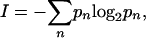[4]

where the logarithm is base two. Information is said to be measured in bits. I is also said to measure the surprise or novelty of an outcome. For the omniscient Court, there is just one outcome, which therefore has probability unity and I_u = 0 bits. There is zero surprise or novelty, because the outcome of the judicial issue does not figure in our deliberations. On the other hand, the platonic Court has 2⁸ possible outcomes, all equally probable, and therefore, in agreement with Eq. 4, I_P = 8 bits of information are revealed when an opinion is handed down. More generally, we will take I + 1 as determining the effective number of justices in the operation of the Court.

The Second Rehnquist Court

Statistics on Court decisions can be found in a number of locations (13, 14). For example, the Harvard Law Review furnishes tables on voting alignments and average actions of individual justices on a term basis. The Harvard Law Review includes among its concerns the opinion-making process; e.g., their tables do ``not treat two justices as having agreed if they did not join the same opinion even if they agreed in the result (14).'' For present purposes, such distinctions will be overlooked. Our sole criterion will be whether a justice does or does not join in the Court's opinion.

The ensemble of decisions for the 8-yr period 1995–2002 derives from the 468 admissible opinions. Nine-dimensional decision space contains just 256 points (Eq. 1), and some decisions therefore must be visited more than once. Table 1 accounts for the 12 most frequent decisions, 377 in number. All other decisions occurred <1% of the time.

Table 1. Most frequent decisions of the second Rehnquist Court.

Br	Gi	Ke	O'C	Re	Sc	So	St	Th	Margin	Frequency, %
1	1	1	1	1	1	1	1	1	9	47 (220)
-1	-1	1	1	1	1	-1	-1	1	1	9.6 (45)
1	1	1	1	1	1	1	-1	1	7	4.5 (21)
1	1	-1	1	-1	-1	1	1	-1	1	3.8 (18)
1	1	1	1	1	-1	1	1	-1	5	3 (14)
1	1	1	1	-1	-1	1	1	-1	3	2.6 (12)
1	-1	1	1	1	1	1	-1	1	5	2.4 (11)
-1	1	1	1	1	1	1	-1	1	5	1.9 (9)
1	1	1	-1	-1	-1	1	1	-1	1	1.9 (9)
1	1	1	-1	1	-1	1	1	-1	3	1.5 (7)
1	-1	1	1	1	1	-1	-1	1	3	1.3 (6)
1	1	-1	1	1	-1	1	1	-1	3	1.1 (5)

Br, Breyer; Gi, Ginsburg; Ke, Kennedy; O'C, O'Connor; Re, Rehnquist; Sc, Scalia; So, Souter; St, Stevens; Th, Thomas.

Unanimous decisions denoted by U occur 47% of the time, whereas the particular five to four majority, denoted by P, accounts for almost 10% of the rulings. The next most frequent accounting for almost 4.5% of the decisions is noteworthy. Of the nine possible eight to one decisions (margin 7), in which one justice dissents, Justice Stevens was the sole dissenter 21 times. Rehnquist, Scalia, and Thomas were each sole dissenters three times, and Breyer, Ginsburg, Kennedy, and O'Connor, each sole dissenters just once. Justice Souter was never the sole dissenter: the decision [1, 1, 1, 1, 1, 1, –1, 1, 1] was never visited in this 8-yr period. In fact, a total of 181 possible decisions were never visited in the course of the 8-yr period 1995–2002. Furthermore, 45 decisions were visited only once, 0.2% of the time, and if we regard these as (ignorable) outliers, just 30 decisions can be regarded as significant in the sense that they were visited more than once.

On the basis of the probabilities of occurrence of the decisions of the present court, we can calculate the information, (Eq. 4). From Table 1 and the additional vote probabilities, it is determined that each time a ruling is handed down by the present Court, I_R = 3.68 bits of information are conveyed. This value lies between I_O = 0 bits and I_P = 8 bits and implies that, in effect, the Court acts as if composed of 4.68 platonic justices.

Venturing into interpretation, one might suppose that in the 220 unanimous decisions, some (abstract) threshold was not reached, so ideology did not play a role, and the Court then behaved according to the omniscient model. Another supposition (not in conflict with the first) might be that the justices did not really rise to omnipotence in the U cases, but that these cases were ``no brainers,'' which in a more efficient system would not have reached the Supreme Court. To pursue this further requires the reasons, possibly manifold, why the Court decides to rule on what will become a U decision.

Some insight into the likelihood of decisions can be gleaned from the joint probabilities that two justices will agree on a decision. Because Table 1 informs us that any two justices agree at least 47% of the time, joint probabilities are displayed in complementary form, namely, the probability that two justices disagree, shown in Table 2. Thus, the least probable event is that Justices Scalia and Thomas disagree, 6.6%, and the next most unlikely event is that Justices Ginsburg and Souter disagree, 9.6% of the time.

Table 2. Joint probability for disagreement for the second Rehnquist Court.

	Br	Gi	Ke	O'C	Re	Sc	So	St	Th
Br	0	0.11966	0.25	0.2094	0.29915	0.35256	0.11752	0.16239	0.35897
Gi	0.11966	0	0.2671	0.25214	0.30769	0.36966	0.09615	0.1453	0.36752
Ke	0.25	0.26709	0	0.15598	0.12179	0.18803	0.24786	0.32692	0.17735
O'C	0.2094	0.25214	0.156	0	0.16239	0.20726	0.22009	0.32906	0.20513
Re	0.29915	0.30769	0.1218	0.16239	0	0.14316	0.29274	0.40171	0.13675
Sc	0.35256	0.36966	0.188	0.20726	0.14316	0	0.33761	0.43803	0.06624
So	0.11752	0.09615	0.2479	0.22009	0.29274	0.33761	0	0.1688	0.3312
St	0.16239	0.1453	0.3269	0.32906	0.40171	0.43803	0.1688	0	0.4359
Th	0.35897	0.36752	0.1774	0.20513	0.13675	0.06624	0.3312	0.4359	0
Dissent	1.86966	1.92521	1.735	1.74145	1.86538	2.10256	1.81197	2.40812	2.07906

See Table 1 for key to abbreviations.

Alternatively, Justices Scalia and Thomas agree >93% of the time, and Justices Ginsburg and Souter >90% of the time. Column sums (shown) are an index of dissent. Thus, Justice Stevens is the most likely to disagree with the other justices, whereas Justices Kennedy and O'Connor are the most likely to be in agreement with their colleagues. The total number of dissents of each justice is given by D = [88, 100, 53, 52, 78, 107, 87, 136, 102], under the convention given in Eq. 1. Thus Justice Stevens cast by far the most, whereas Justices Kennedy and O'Connor cast the fewest dissents. Another interpretation of the latter remark might be that Justices Kennedy and O'Connor are the likeliest to determine the majority opinion, a view supported by Table 1. Of the 72 margin 1 (five to four) decisions shown there, one or both of these justices might be regarded as casting the deciding vote.

Singular Value Decomposition

Each decision has been depicted as a point in nine-dimensional Court space (Eq. 1) but this may not be the best representation. By well defined mathematical criteria, SVD furnishes the optimal coordinate system with which to view data. What this means will become clearer in the following. More detailed mathematical considerations appear in the Appendix.

The ensemble of all decisions can be put into the form of a matrix

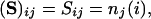[5]

where rows i = 1, 2,..., 468 index the decisions and columns j = 1, 2,..., 9 follow the convention adopted in Eq. 1 for voting. An SVD analysis subsumes the calculation of all correlations of voting alignments among all justices. This information generates new coordinate directions, dictated by the data, which are ordered by degree of importance. The first direction reflects the most frequent voting alignment, the next direction is the second most likely alignment, under the condition that it be orthogonal to the first, and so forth, thus leading to a full set of characteristic directions or vectors. It is also conventional to specify directions by vectors of unit length. Thus, if we denote the characteristic vectors by {V_j}, j = 1, 2,..., 9, and if the elements of V_j are denoted by V_j(k), then where the inner product, denoted by a dot, is defined by the summation and δ_ij is zero for i ≠ j and 1 for i = j. These characteristic vectors, ordered by decreasing importance, are the columns of Table 3. Any decision, n, can be exactly expressed in these terms by .

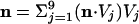Table 3. Characteristic voting vectors and weightings for the second Rehnquist Court.

W1	W2	W3	W4	W5	W6	W7	W8	W9
0.570925	0.218552	0.051724	0.040329	0.033949	0.025719	0.024656	0.019724	0.014422
V1	V2	V3	V4	V5	V6	V7	V8	V9
0.341083	-0.327401	-0.122481	0.242601	0.142766	0.818428	0.037204	-0.020455	-0.102976
0.332609	-0.367567	0.110215	0.073447	-0.427827	-0.193473	-0.212646	0.685597	-0.031553
0.363366	0.174192	-0.346174	-0.579431	-0.101478	0.039381	0.583564	0.165764	0.04661
0.362987	0.104212	-0.527083	0.382865	0.51364	-0.384338	-0.103697	0.103361	-0.000622
0.346547	0.304502	-0.221575	-0.255128	-0.335368	0.10267	-0.665052	-0.327666	0.018063
0.312679	0.403145	0.458959	0.168381	0.114938	0.115622	0.047714	0.122879	0.675836
0.348709	-0.3127	0.075215	0.295861	-0.366213	-0.300389	0.330139	-0.587015	0.0975
0.264479	-0.445911	0.34732	-0.511823	0.509594	-0.166624	-0.191138	-0.155812	0.018946
0.315957	0.405752	0.434937	0.102405	0.054563	-0.039616	0.109552	0.007046	-0.720612

Above each vector (column) of Table 3 is the weighting, w_j, j = 1,... 9, which gives the probability with which a decision lies in the corresponding direction V_j and hence measures its importance. The third highest probability, w₃, is more than an order of magnitude smaller than w₁, which implies that we might approximate decision space, as embodied by S, by just two directions,

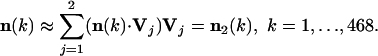[6]

The implication is that the decision space of the Rehnquist Court requires only two dimensions for its description. If true, the will of the Court is embodied in the space spanned by the first two columns of Table 3. (V₁ and V₂ are close, but not the same, in direction as U and P; correlation between V₁ and U is 0.996, and between V₂ and P 0.949; the latter implies an angular separation of ≈18°.) This implies that each justice's vote can be regarded, up to a sign, depending on agreement or disagreement, as a fixed admixture of two voting patterns, V₁ and V₂. Each vote in this approximation represents a balance of these two basic voting patterns.

As a criterion for the evaluation of the 2D approximation, (Eq. 6), we calculate the margin by which a majority is carried. The tenth column of Table 1 gives the true margin, which for the kth decision is .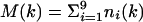

The two-term approximation to the margin is

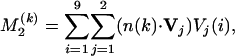[7]

where V_j(i) is the ith component of V_j. The elements of V_j have decimal form, which is awkward, and we round (Eq. 7) to the nearest integer,

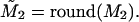[8]

If we carry out this calculation and form the difference, M(k) – M̃₂, we find that this is zero in all but four of the 468 cases. By this criterion, (Eq. 6) is an excellent approximation. (In the Appendix, we demonstrate that this goal of ``goodness of fit'' in fact can be used as a criterion for generating the characteristic directions or votes.) The exceptional cases are shown in Table 4.

Table 4. Aberrant approximations.

Br	Gi	Ke	O'C	Re	Sc	So	St	Th	Margin	M(k) - M̃2	M(k) - M2
-1	1	1	1	1	-1	1	-1	-1	1	2	1.562244
1	1	1	1	1	-1	1	-1	-1	3	4	3.641294
1	1	1	1	-1	-1	1	-1	-1	1	2	1.607662

The middle now occurs twice. See Table 1 for key to abbreviations.

The middle case in Table 4 occurred twice. In two cases, rounding gives a margin of 2 and the other, a margin of 4, violating the rule that the margin must be an odd number. In each, the error is small enough to preserve the correct outcome. In two instances of Table 4, Justice Rehnquist breaks with Justices Scalia and Thomas, and in the other, Breyer breaks with Ginsburg and Souter. As implied in Table 2, these are lowprobability occurrences. Alternatively, two of the votes were visited once and the other, twice. The two-term approximation (Eq. 7) is not expected to approximate the class of unvisited decisions, as discussed in the Appendix.

Comparison with Two Warren Courts

The analysis just presented implies that the U.S. Supreme Court functions in a subspace smaller than nine-dimensional space. Over the 8-yr period followed here, only a small fraction of the 256 possible decisions was visited. Information theory implies that the Court operates, in effect, with 4.86 ideal justices. Decision margins suggest that an essentially 2D description expresses the will of the Court.

It is therefore of interest to make comparisons, and we consider the Warren Courts of 1959–1961 and 1967–1969.

A principal reason for choosing the Warren Courts for comparison is the widely held view of a strong contrast in the inclinations of the Rehnquist and Warren Courts (9). Among other distinctions, the present Court is said to be conservative (vs. liberal) in Constitutional interpretation and inclined toward weak (vs. strong) federal controls. In point of fact, the first of the Warren Courts was not really dissimilar ideologically and, as will be seen, was astonishingly similar to the Rehnquist Court. The greater contrast is really with the second Warren Court, where interesting parallels again exist but are of a more subtle sort.

The 1959–1961 Court was composed of:

(For reasons that will become clear, these justices have not been arranged in alphabetical order.) For the indicated period in which these justices served, we obtained 233 (of 650) admissible decisions.∥

This W1 court voted unanimously ≈33% of the time, in contrast to 47% of the Rehnquist Court. The five to four majority, earlier denoted by P, was visited almost 13% of the time, which is comparable to 10% for the Rehnquist Court. Clearly, a reason for the above arrangement of the Warren Court justices, W1, was to facilitate this comparison. However, there are 2,880 permutations of the entries of W1 that give P, the second most frequent Warren Court ruling. The actual choice of ordering of W1 was dictated by the subsequent SVD. This analysis again reveals that there are just two dominant voting directions, denoted by and . The ordering in W1 was chosen to maximize the correlation of these with their counterparts from the Rehnquist Court. In fact, with our choice, we find that 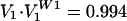and 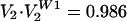, exceptionally high correlations. The chosen W1 provides a mapping of the justices of the two Courts, R↔W1, that reveals a similarity in their complexions and workings. Inspection of R↔W1 makes for some curious identifications, on which I will not comment.

A difference in the Courts is that 73% of the variance is captured by the first two components for the Warren Court, in contrast to 79% for the Rehnquist Court. As a result, a 2D approximation for Warren Court decisions does not do as well as for the Rehnquist Court. Eight minor errors of the previous sort now occur in calculating the two-term approximation to the margin, a 3.5% error compared to the 1% error of Table 4. Along similar lines, the Warren Court visited 56 different decisions in handing down 233 decisions, proportionally more by 33% than the 75 visited by the Rehnquist Court in their 468 decisions. Finally, the novelty of a ruling by this court was I_W1 ≈ 4.1632 bits, larger than I_R = 3.68 bits, implying that this Warren Court operated in effect with 5.16 platonic justices.

Certain other similarities also might be of interest. The third most frequent vote, 4.7%, was the eight to one majority in which Douglas was the sole dissenter, closely paralleling the eight to one majority, 4.5%, occurring when Stevens was the sole dissenter. In total, Douglas dissented ≈35% of the time, whereas Stevens did so ≈30% of the time. Another interesting parallel, already foreshadowed by the R↔W1 mapping, is that Clark and Stewart each voted with the majority ≈86% of the time, thus playing a role similar to that of Kennedy and O'Connor, who voted with the majority ≈90% of the time.

The 1967–1969 Warren Court was composed of:

The six carryover justices have been italicized. For the period in which the Court was composed of these justices, we obtained only 85 admissible cases. (In addition to what has been said before, absences of one or more justices were very significant factors for this period.) Again, U was the most frequent vote, 40%; however, the second most frequent vote, 7%, was a seven to two vote in which Harlan and Stewart dissented, and the third most frequent vote, 6%, was a six-to-three vote in which Black, Harlan, and White dissented. Twenty-nine decisions were visited by this Court, which is proportionately more than the R or W1 Courts. A five to four majority occurred infrequently, only four times, and each occurrence had a different composition. In spite of this divergence with the R and W1 courts, SVD analysis reveals two dominant components, and , which capture 73% of the variance. is similar to a U vote and even though single five to four decisions were seldom or not visited, V^W2 is of this general form (with Black, Harlan, Stewart, and White in the minority). In fact, 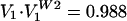and , so that W₂↔R is well correlated. Thus, from the perspective of voting margins, each vote cast again appears as an admixture of a U- and a P-like pattern. For this Warren court, I_W2 ≈ 3.717 bits and 4.717 platonic justices.

It is both diverting and interesting to directly compare the two Warren Courts, W1 and W2. In fact, the mapping W1↔W2, which is the optimal transformation of the two Courts, shows that each carryover justice plays a new role in the altered court. Metaphorically (and literally), under this map, black goes to white. Douglas, Warren, and Brennan, all belonging to the minority in five to four decisions of W1, become part of the ``five to four'' majority of W2, and Harlan, Stewart, and Black go from the majority to the minority. Harlan went from dissenting 20% to 34%, whereas Douglas went from 35% to 14%. A very remarkable aspect of the W2 Court is that Marshall dissented only once (which might be interpreted as indicating a leadership role), and Warren and Brennan did so only three times each.

Comments

The three Courts we have focused on all share the feature that their decisions, in terms of margins, are well described by a 2D space that bears a strong correlation to U and P. At the risk of extrapolating from small statistics, one can speculate that the strong correlations of these dominant patterns might, be dictated in part by a sameness in the overall quality of cases percolating up to the Court through the judicial substructure; and also, perhaps, a dynamic generated by the Court size itself.

In another vein, both SVD and information theory suggest that Court coalitions reduce the dimension of the Court from its potential of nine. The information dimension, which is the better measure of judicial independence, appears to lie between 4.5 and 5. Although this is much smaller than nine, it is significantly higher than a dimension of one, which would be the case if all decisions depended only on a liberal vs. conservative axis. By contrast, in considering the U.S. Congress, Poole and Rosenthal (15) demonstrate, by different methods, that each of our (435) congressmen's votes is located in a 2D space (16). From the perspective of information theory, there is much less ``novelty'' in the outcome of a congressional vote than in a Supreme Court decision. Information theory (Eq. 4) states that the former is potentially enormously larger than the novelty of the latter. The notion of novelty should be balanced by the observation that nine monkeys, trained to flip coins, would render decisions on this basis having the highest novelty.

Appendix

We briefly review some elements of SVD in the context of this paper.

The matrix of decisions, S_ij = n_i(j), is defined by Eq. 5. The search for a unit vector V, such that ∥SV∥² is a maximum, leads to the eigen (characteristic) equation, S^†SV = λV, where † denotes adjoint; e.g., this generates the nine-orthonormal characteristic voting directions (eigenvectors) {V_n} shown in Table 3. The weightings in that table are given by w_j = λ_j/Σ_k λ_k. All eigenvalues are nonnegative, and the solution to the stated maximization problem is V₁ if eigenvalues are arranged in descending order. V₂ solves the same maximization problem, with the added constraint that V₁·V₂ = 0, and so on.

We can connect SVD to the demand that an approximate form, Eq. 6, of {n_i(k)} should closely fit the true voting margin, M(k). For this purpose, it will suffice to consider a one-term approximation to n(k). If V is an as-yet unknown unit vector, we approximate each n(k) by n(k) ≈ (n(k)·V)V, where we have made use of the fact that projection gives the best coefficient. Therefore, we demand that the average overall k of 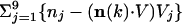for ∥V∥ = 1 be close to zero. A straightforward minimization is complicated by the fact that each sum can be negative, which can lead to an erroneous (negative) minimum. Therefore, we replace this criterion with minimization of Σ_j (n_j(k) – (n(k)·V)V_j)², subject to ∥V∥ = 1. But this summation is equal to ∥n(k)∥² – (n(k), V)², and therefore minimization of the summation is equivalent to maximizing (n(k)·V)². However, this is equivalent to maximizing ∥SV∥², which is just the condition that yields SVD.

Another approach to treating the data looks at the departure of each decision from the averaged vote. When the same SVD analysis is applied to the mean subtracted data, the procedure is called principal components analysis (PCA) (G. W. Stewart, ref. 17). For this reason, the two terms are sometimes used interchangeably. Besides the awkwardness of speaking of departures from an average vote, the resulting PCA analysis is less efficient; it requires an additional characteristic vector to achieve the same margin criterion (Eq. 6) (because the lead SVD direction and the mean are not sufficiently close).

Next, we consider the two-term approximation, n₂(k) (Eq. 6), for the Rehnquist Court. Fig. 1 contains the projection of all points of the decision sphere onto the (V₁, V₂) plane, where V₁ is the vertical and V₂, the horizontal direction. The coordinates of each decision are given by n₂(k) = (n(k)·V₂, n(k)V₁), k = 1,..., 256. The semicircles represent R₂ = 2 and R₂ = 3, where 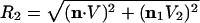, a nominal choice for an annulus in which n(k), is well approximated by n₂(k). The asterisks (*) mark the 18 most frequent voting alignments, accounting for 397, or 85%, of the rulings. The uppermost (*) corresponds to U and the rightmost, to P. The open circles (○) denote the next 12 most frequent rulings, and pluses (+) denote once-visited votes. The 181 dots (•) represent unvisited voting alignments. There are some striking features of Fig. 1, and we comment on a few.

1. Many votes, ○ and +, lie inside R₂ < 2, where n₂(k) is a poor approximation to n(k), but for which the approximate margin, (Eq. 8), is correctly given. To account for this, we recall that the margin is obtained by summing the individual votes of the justices and so is like an average. The process by which characteristic directions are obtained, as discussed above, overlooks individual errors in favor of obtaining a good approximation to the average. The dashed arrow to the upper asterisk is significant, because the inner product of this vector with a vector to any symbol gives M₂(k) (Eq. 7) of the corresponding ruling.

2. There are a number of once-visited rulings (+) that lie well in the annulus 2 < R₂ < 3. Four of these are eight to one rulings, and another is [1, 1, –1, –1, 1, –1, 1, 1, –1]. Analysis implies that such rulings are well within the framework of the Court. The unanswered question is, ``Why are there not more cases that produce these alignments?''

3. Similarly, in considering the unvisited votes (dots) we find that [–1, 1, 1, 1, 1, 1, –1, –1, 1], [–1, –1, 1, 1, 1, 1, 1, 1, 1], and [1, 1, 1, 1, 1, 1, –1, 1, 1] are all within the annulus. Why were there no cases to produce such alignments, when analysis suggests they are within the Court's framework?

Fig. 1.

2D projection of the second Rehnquist Court. V₁ is the vertical and V₂, the horizontal direction. The inner product of heavy dashed vector with vector to any point generates M₂(k) (Eq. 7). *, ○, and +, visited rulings. •, unvisited rulings (see text).

References

- 1.Greenhouse, L. (October 6, 2002) N.Y. Times, Sec. 4, p. 3, col. 1.
- 2.Strang, G. (1988) Linear Algebra and Its Applications (Harcourt Brace Jovanovich, San Diego), 3rd Ed.
- 3.Sirovich, L. & Everson, R. (1992) Int. J. Supercomput. Appl. 6, 50–68. [Google Scholar]
- 4.Taylor, A. D. (1995) Mathematics and Politics: Strategy, Voting, Power and Proof (Springer, New York).
- 5.Epstein, L. & Knight, K. (1997) The Choices Justices Make (Congressional Quarterly, Washington, DC).
- 6.Hall, K. L., ed. (1992) The Oxford Companion to the Supreme Court of the United States (Oxford Univ. Press, Oxford).
- 7.Hall, K. L., ed. (1999) The Oxford Guide to United States Supreme Court Decisions (Oxford Univ. Press, Oxford).
- 8.Rehnquist, W. H. (2002) Supreme Court (Knopf, New York).
- 9.Starr, K. W. (2002) First Among Equals: The Supreme Court in American Life (Warner, New York).
- 10.Segal, J. A. & Spaeth, H. J. (2002) The Supreme Court and the Attitudinal Model Revisited (Cambridge Univ. Press, Cambridge, U.K.).
- 11.Hilbert, D. & Cohn-Vossen, S. (1999) Geometry and the Imagination (Am. Math. Soc., Providence, RI).
- 12.Pierce, R. (1980) An Introduction to Information Theory (Dover, Mineola, NY).
- 13.Quain, A., ed. (2002) The Political Reference Almanac (Keynote, Arlington, VA), 2001–2002 Ed.
- 14.The Harvard Law Review Association (November, 1994) Harvard Law Review, Vol. 108.
- 15.Poole, K. T. & Rosenthal, H. (2000) Congress: A Political–Economic History of Roll Call Voting (Oxford Univ. Press, Oxford).
- 16.Krugman, P. (October 20, 2002) N.Y. Times, Sec. 6, p. 62, col. 1.
- 17.Stewart, G. W. (1993) SIAM Rev. 35, 551–566. [Google Scholar]
- 18.Martin, A. D. & Quinn, K. M. (2002) Polit. Anal. 10, 134–153. [Google Scholar]