Use of Stimulus-frequency Otoacoustic Emission Latency and Level to Investigate Cochlear Mechanics in Human Ears

Abstract

Stimulus frequency otoacoustic emission (SFOAE) sound pressure level (SPL) and latency were measured at probe frequencies from 500 to 4000 Hz and probe levels from 40 to 70 dB SPL in 16 normal-hearing adult ears. The main goal was to use SFOAE latency estimates to better understand possible source mechanisms such as linear coherent reflection, nonlinear distortion, and reverse transmission via the cochlear fluid, and how those sources might change as a function of stimulus level. Another goal was to use SFOAE latencies to noninvasively estimate cochlear tuning. SFOAEs were dominated by the reflection source at low stimulus levels, consistent with previous research, but neither nonlinear distortion nor fluid compression become the dominant source even at the highest stimulus level. At each stimulus level, the SFOAE latency was an approximately constant number of periods from 1000 to 4000 Hz, consistent with cochlear scaling symmetry. SFOAE latency decreased with increasing stimulus level in an approximately frequency-independent manner. Tuning estimates were constant above 1000 Hz, consistent with simultaneous masking data, but in contrast to previous estimates from SFOAEs.

I. INTRODUCTION

A. Sources of SFOAEs

Stimulus frequency otoacoustic emissions (SFOAE) are generated in the cochlea in response to sound. They can be generated by continuous tones, or primaries, of frequencies f₁ and f₂ presented at levels L₁ and L₂, respectively, and the SFOAE is recorded at either of the primary frequencies. Another way to specify the primaries is “probe” and “suppressor,” meaning the SFOAE is recorded at the frequency of the probe that is presented in the presence of a suppressor. A review of the methods for extracting SFOAEs can be found in Schairer et al. (2003). The goals of this study are to measure SFOAE latency as a function of both stimulus frequency and level, to evaluate alternative source mechanisms of SFOAEs, and to use SFOAE latencies to indirectly estimate cochlear tuning using the SFOAE-source theory of linear coherent reflections.

Two theories based on forward and reverse transmission of mechanical energy along the basilar membrane (BM) have been proposed to account for the generation of SFOAEs. The first theory is linear coherent reflection (Shera and Guinan, Jr., 2003; Shera and Zweig, 1993; Zweig and Shera, 1995). This theory predicts that at low levels, SFOAEs are generated by coherent (i.e., phase-sensitive) reflections from a random distribution of impedance irregularities along the BM. Thus, the SFOAE measured at the probe frequency is dominated by energy reflected from impedance irregularities at the peak of the traveling wave near the tonotopic place of the probe frequency. The linear coherent reflection mechanism centers on the cochlear mechanics at the limit of low stimulus levels [below approximately 20 dB sound pressure level (SPL)] where the outer hair cell (OHC) functioning is linear (Zwicker, 1983; Zwicker and Schloth, 1984). However, it is important to note that the basic mechanism of linear coherent reflection is a linear scattering of the forward traveling wave along the BM due to a distribution of inhomogeneities in transmission characteristics. This basic “linear” mechanism is assumed present even at moderate and high stimulus levels in which the compressive nonlinearity of BM mechanics limits the growth of response near tonotopic place. The second theory posits that, in response to a sinusoidal excitation, a nonlinear distortion component is created on the BM, which thereby acts as a SFOAE source at the probe frequency (Brass and Kemp, 1993). Irrespective of the generator mechanism, a nonlinear SFOAE residual is measured using a “suppression paradigm,” in which the presence of a second sinusoidal tone is assumed to suppress the traveling wave on the BM at the probe frequency, and this suppressed response is compared at the probe frequency with the response to the probe tone alone. The nonlinear SFOAE residual may be extracted even if the second tone does not fully suppress the probe tone, however, the maximum emission amplitude will not be produced (because suppression is incomplete), and other nonlinear effects may be produced. Both theories (linear coherent reflection and nonlinear distortion) require normal, active function of the OHC, with its associated nonlinear response growth properties that influence the cochlear mechanics.

A third theory of SFOAE generation is based on forward transmission of mechanical energy along the BM to the tonotopic place, but reverse transmission of the SFOAE through cochlear fluid. Ren (2004) reported data that he interpreted as contradicting theories that stated that the return of energy forming a (DPOAE) is through backward, or reverse, traveling waves. Ren used scanning-laser interferometry to monitor BM vibrations at the f₁, f₂, and DPOAE frequencies (2f₁, f₂) and concluded that only forward traveling waves were observed. Ren suggested that energy is returned to the base of the cochlea through a compression wave in the cochlear fluids, rather than through a reverse traveling wave on the BM, to generate emissions. Such a mechanism might also be present in SFOAE generation. This would contradict the nonlinear-distortion and coherent reflection theories, which are based on a reverse mechanical wave present on the BM. The current SFOAE data were collected with f₂/f₁ of 1.02-1.03, which is similar to the smallest f₂/f₁ ratio of 1.05 that Ren used.

The time it takes for the compression wave to travel from the tonotopic place to the stapes through the cochlear fluid is much shorter than the characteristic forward travel time for the mechanical traveling wave on the BM between stapes and tonotopic place, and is approximated as zero within the limits of our measurement precision. Thus, if SFOAE generation was dominated by this source, the latency of the resulting emission would be approximately equal to the forward travel time on the BM. A level-dependent transition between coherent-reflection emission and the compressional-wave mechanism would be associated with a reduction in SFOAE latency by a factor of approximately one-half.

Although it is generally accepted that SFOAEs are dominated by the linear coherent reflection source at low to moderate stimulus levels (40 dB SPL and slightly higher),it is less clear which source dominates SFOAE generation at higher stimulus levels. The next section describes how the SFOAE latency estimate τ, which is derived from the gradient of the SFOAE phase $\phi \left(f\right)$ by

$$\tau =-(1∕2\pi )d\phi \left(f\right)∕df,$$ (1)

can be used to separate the different sources. Latency estimates are used in the current experiment to characterize changes in dominant sources as a function of stimulus level.

B. Using SFOAE latency estimates to separate sources

In the current study, f₁ is the probe frequency at which the SFOAE is recorded, f₂ is the suppressor frequency, and f₁<f₂. The latency as a function of frequency has been used to separate the different mechanisms in DPOAE, which may be generated near the region of f₂ and a SFOAE in the region of 2f₁-f₂. The DPOAE latency is defined by a relation analogous to Eq. (1), except that $\phi \left(f\right)$ is the phase at the DPOAE frequency as a function of the frequency that is swept. Procedures include sweeping f₂ with a fixed f₂/f₁, sweeping f₂ with a fixed f₁, or sweeping f₁ with a fixed f₂ (Kalluri and Shera, 2001; Knight and Kemp, 2000; Tubis et al., 2000). The resulting DPOAE latency depends on the choice of the frequency sweep procedure. If f₂ is swept at fixed f₂/f₁, then the region of interaction, in relation to f₂ and f₁, will be constant, and the phase of the emission that arises from this region will be nearly constant as a function of f₂. This is reflected as zero group delay from the cochlea, but there may be delays associated with the middle ear and ear canal. Thus, nonlinear distortion sources at 2f₁-f₂ are characterized by short, near-zero latencies that change gradually as a function of frequency. A similar method can be used to separate sources for SFOAEs, based on sweeping the probe tone at f₁ and using a suppressor tone f₂ such that f₂/f₁ is fixed.

The SFOAE phase is predicted to change rapidly as the probe frequency changes according to the linear coherent reflection theory, because the energy is reflected from spatial irregularities at the peak of the traveling wave at the tonotopic place of the stimulus. Thus, linear coherent-reflection sources are characterized by steep phase gradients, and longer latencies that change as a function of frequency.

Multiple internal reflections also contribute to the SFOAE phase, and the individual internal reflections can be separated by time-domain analyses of SFOAE responses (Konrad-Martin and Keefe, 2005). In the bidirectional theory of SFOAE transmission, SFOAEs propagate in the reverse direction from the tonotopic region of the cochlea to the basal end of the cochlea, at which place the SFOAE is partially transmitted through the middle ear into the ear canal and partially reflected to form an internal reflection of the SFOAE. Such an internally reflected SFOAE is proportional to the basal reflectance at the oval window, and propagates in the forward direction to the tonotopic place where it may be rereflected in the reverse direction as an additional component of the SFOAE. This rereflected component is proportional to the apical reflectance. This process of reflections near the tonotopic place and the basal end of the cochlea produces a sequence of multiple internal reflections, such that the total SFOAE signal recorded in the ear canal is a sum of the SFOAE in the absence of such internal reflections and the partially transmitted SFOAE components associated with each internal reflection. If the magnitude of the product of the basal reflectance and apical reflectance is small compared to unity, then the effect of multiple internal reflections on the SFOAE phase can be modeled using a perturbative model. Such a model predicts a quasi-periodic fine structure, in which the phase is the sum of the SFOAE phase in the absence of internal reflections and an oscillatory term (Talmadge et al., 1998; Zweig and Shera, 1995). The product of basal and apical reflectance magnitudes has been measured in a human ear as having an upper bound of 0.125 (Konrad-Martin and Keefe, 2003), which is sufficiently small to validate such a perturbative approach. The methodology described below for the current study smoothes the unwrapped SFOAE phase prior to calculating its phase gradient. This smoothing operation removes the fine structure associated with multiple internal reflections. Therefore, these multiple internal reflections are unlikely to contaminate the SFOAE latency measurements reported herein. In addition, the effects on SFOAEs of multiple internal reflections diminish with increasing level, so that their impact on SFOAE latencies, even if present at low levels, would diminish at higher probe levels.

The original formulation of linear coherent-reflection theory, which was based on one-dimensional BM mechanics, proposed that SFOAE latency is determined by the BM latency (i.e., group delay) at the traveling wave peak (Zweig and Shera, 1995). This one-dimensional theory predicted that the forward and reverse BM travel times were equal. It follows that, except for any short latencies associated with earcanal and middle-ear transmissions, the SFOAE delay is predicted to be approximately twice the travel time to the tonotopic place of the stimulus on the BM. Because the BM is tuned to higher frequencies toward the base and lower frequencies toward the apex, emissions that are dominated by coherent reflection are predicted to have latencies that decrease as frequency increases. These predictions are supported at low stimulus levels (and at least at higher frequencies) in measurements from cats, guinea pigs, and humans (Dreisbach et al., 1998; Shera and Guinan, Jr., 2003). A more recent formulation of the linear coherent reflection theory based on a two-dimensional model of BM mechanics predicts that the SFOAE latency is somewhat less than twice the BM group delay (Shera et al., 2005). Because of the lack of knowledge of BM group delay in human cochleae, the simpler prediction of the one-dimensional formulation of the linear coherent emission theory is mainly used in this report.

One current question is how SFOAE latency varies with stimulus levels, and because SFOAE latencies are expected to be related to BM latencies, it is relevant to consider published data on phase nonlinearity in BM mechanics. The amplitude of BM motion varies with stimulus level according to a compressive nonlinearity (Rhode, 1971). At low levels, the traveling wave peak for a sinusoidal stimulus is sharper than at higher levels, and occurs near the tonotopic or resonant place on the BM that corresponds to the frequency of the stimulus. As stimulus intensity increases, the peak broadens and shifts to a lower frequency. The nonlinearity in the magnitude of BM response to a pure tone is a compressive nonlinearity near the tonotopic place, and this nonlinearity in response magnitude is accompanied by a nonlinearity in the BM phase near the tonotopic place in the basal cochlear region of the squirrel monkey (Rhode and Robles, 1974), guinea pig (Nuttall and Dolan, 1993; Sellick et al., 1982), cat (Cooper and Rhode, 1992), chinchilla (Ruggero et al., 1997), and gerbil (Ren and Nuttall, 2001). Rhode and Cooper (1996) reported a qualitatively similar nonlinear BM phase response in the apical turn of the chinchilla cochlea. For measurements at the best-frequency (BF) place, the main pattern was that the phase at the BF typically varied little with the stimulus level, whereas the phase delay increased with increasing stimulus level at frequencies slightly below BF and decreased at frequencies above BF. This phase pattern is similar to neural patterns observed in single auditory nerve fibers (Anderson et al., 1971), which suggests that BM nonlinearity is the source of this neural nonlinearity. Most of these studies of BM mechanics did not report the change in the slope of the BM phase with the stimulus level, which is needed to predict the latency to the BF place, but the results of all these studies are consistent with a decrease in the BM group delay at BF with an increasing stimulus level. An exception is that of Ruggero et al. (1997), who reported that the BM group delay in the tonotopic region of a 10 kHz tone in one cochlea decreased from 0.99 ms for 10-dB tones to 0.61 ms for 90-dB tones. The ratio of these group delays was approximately 0.6 between the highest and lowest stimulus levels.

If SFOAE latency is closely related to BM motion, as assessed through the group delay at the tonotopic place, then one would expect SFOAE latency to decrease as the stimulus level increases as long as SFOAEs are predominantly generated near the tonotopic place. However, there are complications with this comparison. First, BM measurements are taken at one point on the BM, whereas SFOAEs are recorded in the ear canal. Ear canal measurements of SFOAEs necessarily include reverse-propagation effects. Second, independent estimates of the group delay of the BM traveling wave are not available in human cochleae. These measurements cannot be done in humans, and hypotheses necessarily must rely on estimates from animal models (and possibly damaged cochleae), which may be functionally different than undamaged human cochleae. Thus, measurements of SFOAE latency in human ears provide noninvasive data on BM mechanics that are otherwise unavailable.

Goodman et al. (2003) used the SFOAE phase and time-domain analysis of data recorded in guinea pig ears to determine if variations in the SFOAE level as a function of frequency (i.e., microstructure) were due to variations in reflectance (e.g., impedance irregularities), and/or interference of two sources that varied in phase as a function of frequency (i.e., sources with different latencies). They concluded that SFOAE microstructure is due to a complex addition of two components, one with a slowly rotating phase (the nonlinear-distortion component) and one with a rapidly rotating phase (the linear coherent-reflection component). They stated that other sources were involved, such as variations in reflectance along BM and effects of multiple internal reflections. Linear reflection was described for one example as dominant at most levels, but the nonlinear-distortion component was dominant at a high level (86 dB pSPL).

In the current study, SFOAE latency was estimated at probe frequencies from 500 to 4000 Hz in 16 normal-hearing adult ears, and at probe levels of 40 to 70 dB SPL. Three possible outcomes of the experiment are described in the next section. Because independent estimates of BM travel time cannot be made, it is assumed that the latencies estimated in the lowest probe-level condition are estimates of the round-trip travel time, and that one half of those latencies represent forward travel time.

C. Possible outcomes

One possible outcome would be that SFOAE latency is independent of level. Latencies would decrease as frequency increases in accord with the linear coherent-reflection theory at all probe levels. Latencies would be the same between the 40- and 70-dB SPL probe levels conditions and approximately equal to the round-trip travel time. This would suggest that SFOAEs are dominated by the linear coherent reflection source at higher levels, and that the BM travel time does not change as a function of level in normal human ears.

A second possible outcome would be that SFOAE latencies at high stimulus levels are short (near zero) and independent of frequency, as compared to long, and frequency dependent at lower levels. This would suggest that SFOAEs are dominated by nonlinear distortion at higher levels.

A third possible outcome would be that SFOAE latencies decrease with increasing stimulus level, but remain substantially larger than those expected if SFOAEs were dominated by nonlinear distortion at high levels. This decrease in latency might occur in two ways, one due to BM nonlinearity, and the other due to a level-dependent transition in the reverse BM signal between a mechanically generated transmission at lower stimulus levels and an acoustic compressional wave at higher stimulus levels.

With respect to BM nonlinearity, as reviewed above, the BM group delay decreases with increasing stimulus level. With the view that SFOAEs are generated within the region of the tonotopic place, it would be expected that SFOAE latencies would also decrease with increasing stimulus level. The extent of the change cannot be predicted. However, if SFOAEs are generated at higher stimulus levels by a combination of nonlinear distortion and coherent reflection, as in the theory of Talmadge et al. (2000), then SFOAE latency might decrease as probe levels increase, but to a lesser degree than if nonlinear distortion were the dominant source alone. Influences on OAEs due to nonlinearity associated with the stiffness of the OHC cilia have also been proposed (Liberman et al., 2004).

With respect to the acoustic compressional wave mode, latency would be approximately one half of the latency predicted by the linear coherent-reflection theory. That is, latency would be equal to the time it takes for the traveling wave to peak at the tonotopic place (forward transmission time), because the reverse transmission would be through the fluid with negligible delay. However, the fact that BM nonlinearity also may reduce latency at high stimulus levels suggests that if both these mechanisms were present, the latency might be reduced by a factor even smaller than 0.5.

II. METHODS

A. Subjects

Sixteen adults (8 females, 8 males) ages 19 to 33 years (mean=23.75 years) participated as paid volunteers. The procedures were explained, and each subject signed a consent form before testing began. Subjects had air-conduction thresholds equal to or less than 15 dB (HL) at audiometric test frequencies of 250 to 8000 Hz in the test ear. Air-bone gaps were no greater than 10 dB, and tympanometry using a 226-Hz probe tone suggested normal middle-ear pressure and admittance (ranges: -50 to +35 daPa, 0.3 to 1.5 mL) in the test ear on the day of the test. Subjects were seated in a sound-attenuated booth during OAE testing, and were allowed to sleep or read quietly during data collection.

B. Stimuli and procedure

Stimuli were generated by an in-house software program, using a 24-bit Card Deluxe sound card (Digital Audio Labs) and transmitted to an Etymotic ER-10C low-noise probe microphone and receiver system that was modified to provide an extended 20-dB range of output. Stimuli were presented in a double-evoked procedure (Keefe, 1998) in a set of three intervals defined as follows. Stimulus f₁ was presented in interval one, f₂ in interval two, and both primaries were presented simultaneously in interval three. Responses were also acquired in each of the three intervals. SFOAEs were measured over the frequency range 500-4000 Hz, with separate recording sessions for each octave in the range. A real-time high-pass filter with cutoff frequency f_c was used to attenuate low-frequency noise below f_c, with f_c=250 Hz for measurements between 500 and 1000 Hz, f_c=500 Hz for measurements between 1000 and 2000 Hz, and f_c=650 Hz for measurements between 2000 and 4000 Hz.

The primary frequency ratio (suppressor to probe, or f₂ to f₁) was maintained in the range 1.02-1.03 at 65 frequency steps per octave, with variability in the frequency ratio arising from choosing each frequency from one of the center frequencies of the discrete Fourier transform response (DFT) bins. The sample rate was fixed at 32 000 Hz, but the number of samples differed across the three octaves in order to maintain the same number of frequency steps and similar frequency ratios across the three octaves. The response-buffer size, equal to the number of frequency bins of the DFT, was 4096 samples for SFOAEs from 500 to 1000 Hz, 2048 samples from 1000 to 2000 Hz, and 1024 samples from 2000 to 4000 Hz. The corresponding step size in frequency between adjacent SFOAEs was approximately 8 Hz from 500 to 1000 Hz, 16 Hz from 1000 to 2000 Hz, and 31 Hz from 2000 to 4000 Hz octave. Data were acquired at probe levels (L₁) of 40, 50, 60, 65, and 70 dB SPL, with a suppressor level (L₂) that was always 15 dB above L₁. A suppressor level of 15 dB was chosen because in preliminary studies, it was the best compromise between providing enough suppression to elicit a nonlinear residual across the range of desired L₁ conditions, and producing an adequate signal-to-noise ratio (SNR), which is reduced at higher stimulus levels due to level-dependent variability of the responses. Further, if the suppressor level was much more than 15 dB, it would have restricted the highest level of L₁ that could have been presented due to subject protection issues (i.e., limitation of exposure to loud stimuli) and the fact that probe distortion was observed at higher levels than those used in the experiments. An alternative method to achieve higher probe levels might be to use tone-burst stimuli.

Within each of the three stimulus/response intervals, the buffers just described were repeated six times, and the first two repetitions were discarded to remove stimulus artifact arising from buffer transitions. Between 500 and 1000 Hz, the entire buffer (i.e., set of three intervals) was repeated 16 times, for a total of 64 responses in the average SFOAE. Between 1000 and 4000 Hz, the entire buffer was repeated eight times, for a total of 32 responses in the average. More averaging was used in the lower octave to improve the signal-to-noise ratio (SNR). These procedures are similar in form, if not in exact numbers of repetitions, to procedures described more fully in Schairer et al. (2003).

Data were acquired in the left ear in eight subjects, and in the right ear in eight other subjects. Stimulus levels were varied (i.e., L₁=40-70 dB SPL) at each f₁ before moving to the next f₁. Data were collected over four to six sessions of 1 to 2.5 h each. The entire procedure was repeated in the right ear of subject PH02 and the left ear of subject PH12, with approximately two months between the first and second tests.

C. Analysis

In order to extract the nonlinear residual OAE (P_d) at the probe frequency of f₁, the sound pressure (P₁) was recorded in response to f₁ in interval one, P₂ in response to f₂ in interval two, and P₁₂ in response to the combined presentation of the two stimuli in the third interval. The OAE pressure (P_d) was calculated as follows:

$$P_d=P_1+P_2-P_{12}.$$ (2)

The DFTs of the average pressure wave forms were calculated and evaluated at the probe frequency f₁. Note that although other OAEs are elicited (i.e., at distortion product frequencies), only the data from the frequency bin of the probe are presented. The distortion products and internal reflections may have an effect on the emission recorded at the probe frequency in the ear canal, but those effects were not specifically identified in this analysis. Also note that because the suppressor was always 15 dB above the probe level, full suppression may not have been obtained, particularly at low levels. The noise level (SPL) was calculated as the standard error of the responses across the repetitions of the entire buffer (Schairer et al., 2003). System distortion was estimated by presenting the experimental conditions in a Bruel and Kjaer Ear simulator (coupler) Type 4157 (IEC 711 standard).

The SFOAE phase (at f₁) was calculated relative to the probe-stimulus phase as the phase of the SFOAE P_d (at f₁) minus the phase of the P₁ stimulus (at f₁). At each probe level, the resulting phase spectrum over frequency was unwrapped. A problem is that phase unwrapping is sensitive to the presence of noise, and any such errors in phase unwrapping introduce discontinuities in the phase gradient, and hence in SFOAE latency. To avoid this problem, Shera and Guinan (2003) included only SFOAE phase data at which the SNR>15 dB. Discontinuities in the phase gradients remained in the current data after imposing this SNR criterion. Shera and Guinan used a three-point interpolation to calculate a phase gradient, and hence a latency. To reduce noise, Shera and Guinan used a locally weighted scatter plot smoothed (loess) technique to calculate a latency estimate across subjects that varied smoothly with frequency. There is a tradeoff in requiring a higher SNR in order to have a smoother phase, and the fact that the range of SNR in SFOAE responses is limited. An alternative phase-smoothing technique was used in the current study to calculate SFOAE latencies, and is described after presenting the SFOAE phase results.

III. RESULTS

A. SFOAE level

The repeatability of individual-ear responses is first described. For subjects PH12 and PH02, Figs. 1 and 2 show the SFOAE level measured in two runs as a function of f₁ and as a function of L₁ from 70 to 40 dB SPL from the top to the bottom rows. The solid lines represent the emissions and the dashed lines represent the noise. The gray shading represents the region between the distortion and noise recorded in an IEC 711 standard coupler. Any emissions that fall into this region are questionable.

FIG. 1.

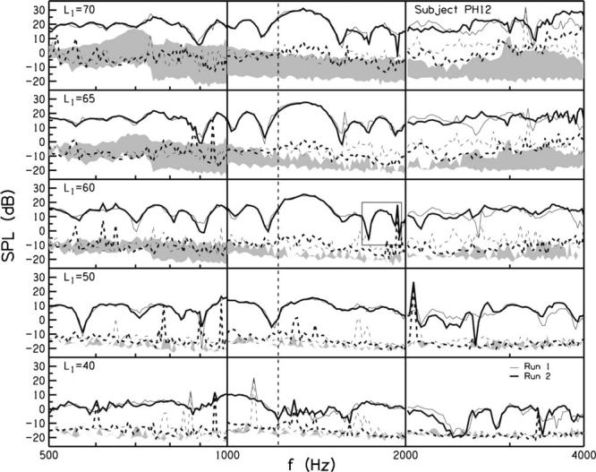
Repeatability for SFOAE level in decibel SPL as a function of the probe frequency (f₁) in hertz for example subject PH12. The suppressor frequency (f₂), number of samples, and the number of stimulus repetitions were different across the three octaves, and were selected to maintain a f₂/f₁ratio of 1.02-1.03 for 65 frequency steps per octave with a constant signal-to-noise ratio. Probe levels (L₁) of 70 to 40 dB SPL are shown in the different rows, top to bottom. Suppressor levels (L₂) were 15 dB above L₁.The thin lines represent run 1, and thick lines represent run 2, which was obtained about two months after the first run. The solid lines represent emission level, and the dashed lines represent the noise (or variability of the response). The shaded regions denote the area between the distortion and noise recorded in a coupler. The root-mean-square (rms) errors between emission levels from runs 1 and 2 were calculated across the three octaves in each condition, and they are shown in Table I. The vertical dashed line is centered on a minimum in the lowest L₁ condition, to help the reader see the shift in the minimum to lower frequencies as L₁ increases. The responses in the square in the L₁=60 condition are described in the text for a comparison to the phase plots in Fig. 3.

FIG. 2.

Repeatability of SFOAE SPL for subject PH02 in the same format as for Fig. 1.

Noise level increased with increases in level for both subjects. This is consistent with previous studies that demonstrated stimulus level-dependent variability in input-output functions at probe frequencies of 1000, 2000, and 4000 Hz (Schairer et al., 2003; Schairer and Keefe, 2005). This stimulus level-dependent increase in noise was not observed in the coupler. The shaded areas increased with increasing level because the distortion recorded in the coupler increased without a corresponding increase in noise level.

The fine structure, i.e., the pattern of maxima and minima in SFOAE level, in PH12's ear was repeatable in general in run 1 (thin line) and run 2 (thick line), although less repeatable between 2000 and 4000 Hz. The linear coherent-reflection theory predicts that minima in the SFOAE level occur because wavelets that are scattered from random spatial fluctuations, and that vary in phase, cancel each other to varying degrees at different frequencies (Zweig and Shera, 1995). Although DPOAE fine structure increases with decreasing stimulus level (He and Schmiedt, 1997; He and Schmiedt, 1993), such a trend in SFOAE fine structure was not clearly observed in the current study.

For subject PH12, the minima tended to move to lower frequencies as L₁ increased. The dashed vertical line is centered at a minimum in the L₁=40 condition as a guide to show how the minimum gradually shifted to lower frequencies with increases in L₁. The SNR was repeatable except for a few sharp maxima in the noise floor (perhaps when the subject moved), and the higher noise level in run 1 across the 2000-4000 Hz range. The presence of noise peaks, such as around 2000 Hz in the L₁=50 condition where SNR becomes 0, was associated with a discontinuity in SFOAE phase and hence latency.

The fine structure for PH02 was repeatable and did not decrease with decreasing stimulus level as much as for PH12. The minima in the fine structure also did not show the same trend toward lower frequencies with increasing level, as seen in PH12. Differences in noise in one octave relative to the others may have occurred because each octave was recorded in a separate session. However, the noise was larger in the 1000 to 2000 Hz range for both runs (relative to the flanking frequency ranges) in subject PH02. If the increased noise were due to changes in subject state or poor probe fit, it would not be expected to be repeatable. Because it was repeatable, it suggests that this ear may be more susceptible to level-dependent response variability in the 1000-2000 Hz range.

Repeatability was quantified by calculating the root-mean-square (rms) error of the SNR (in decibels) across the two runs summed over all frequencies in each L₁ condition Table I shows the rms error in all conditions for both subjects (with minimum and maximum levels in bold italics). The errors in SNR ranged from 4.46 dB for subject PH02 in the L₁=40 condition to 8.55 dB for the same subject in the L₁=60 condition. An important contributor to this error was the presence of large noise spikes at a few frequencies. The noise spikes were most likely due to subject movements that momentarily increased the variability of the response. Once the variability increased, there were not enough stimulus presentations to average out the variability for that particular data point.

TABLE I.

Subject	L1 condition	RMS error in dB of SNR run 1 vs run 2	RMS error in cycles of phase run 1 vs run 2
PH02	40	4.46	1.32
	50	6.55	1.01
	60	8.55	0.10
	65	8.28	0.71
	70	7.21	0.64
PH12	40	5.30	0.12
	50	5.83	1.06
	60	7.03	0.28
	65	7.05	0.88
	70	6.96	0.30

B. SFOAE phase

Figures 3 and 4 show repeated measurements of the unwrapped SFOAE phase spectra for subjects PH12 and PH02. Parameters are represented as in Figs. 1 and 2, except in Figs. 3 and 4, the dashed lines represent the phase estimated from the coupler measurements. As expected, there was no frequency or level dependence of phase in the coupler. In each subject's ear, the SFOAE phase decreased with increasing frequency, and its phase gradient became shallower as L₁ increased.

FIG. 3.

Repeatability for SFOAE phase for subject PH12 as a function of f₁.Parameters are represented as in Fig. 2, except in this figure, the dashed lines represent the phase estimated from the coupler measurements. The rms errors between phase from runs 1 and 2 in each condition are shown in Table I. The phase measurements in the square in the L₁=60 condition are described in the text for comparison with the level measurements in Fig. 1.

FIG. 4.

Repeatability for SFOAE phase for subject PH02 in the same format as Fig. 3.

The SFOAE phase differed across the two runs at frequencies in which the SNR was reduced by noise spikes. However, the SFOAE phase difference between the two runs was sometimes small even at frequencies where the SNR was small. For subject PH12, in the L₁=60 condition over a range from 1000 to 2000 Hz, there was a sharp notch in emission level (see square in Fig. 1), but there was a difference in SNR across the two runs because the noise was larger in run 1. The corresponding SFOAE phases (see square in Fig. 3) deviated from each other. At a slightly higher frequency, there was a peak in the noise for run 2 and (coincidentally) a notch in emission level in run 1, and the SFOAE phases in overlapped again. This is similar to the steps in phase corresponding to minima in the amplitude microstructure observed in guinea pig (Goodman et al., 2003).

The rms errors in SFOAE phase from runs 1 and 2 were calculated across the three octaves, and are shown in Table I. The rms errors ranged from 0.10 cycles in the L₁=60 condition for subject PH02 to 1.32 cycles in the L₁=40 condition for the same subject. A rms phase error of one or more cycles likely corresponds to an effect of noise in the phaseunwrapping operation.

It might be expected that the smallest SNR error would be associated with the smallest rather than the largest phase error. A comparison of the emission level (Fig. 2) and phase (Fig. 4) for this subject explains the trend. In the L₁=40 condition in Fig. 2, there was a sharp notch in emission level for both runs near 640 Hz, and a peak in the noise at a slightly higher frequency for run 1. Otherwise, the SNR was similar across the three octaves for both runs. In the phase plot for the corresponding condition in Fig. 4, there was a deviation in the phase near 640 Hz, which is likely associated with the noise spike in the SNR. Such a spike would produce an error in the phase unwrapping that might influence all higher frequencies, thus leading to a large rms phase error, as was observed. The effect of the noise spike at 640 Hz would produce only a localized spike in the SFOAE latency near 640 Hz.

C. Spline method to smooth SFOAE phase

SFOAE latency was calculated using two approaches in this study using different subject inclusion criteria. These approaches were to (1) unwrap phase, estimate the latency in each ear from phase gradients based on a three-point-finite-difference method, and smooth latency across frequency using a loess approach or (2) unwrap phase, smooth the phase across frequency for each ear using a smoothed cubic-spline interpolation, and then calculate latency as the derivative of the spline function. The first approach replicated the method of Shera and Guinan (2003). Because the calculation of the phase gradient is highly sensitive to noise, Shera and Guinan used an inclusion criterion that the SFOAE SNR exceed 15 dB. Our simulations for a tone in Gaussian noise showed that smaller SNR criteria than 15 dB were inadequate for extracting the signal phase gradient from noise at the frequency of the tone, and that even a 18 dB SNR criterion might be advisable. However, an inclusion criterion of 15 dB SNR may exclude many SFOAE responses, e.g., at frequencies where the noise is high, the stimulus level is low, or near a minimum in the fine structure of the SFOAE SPL.

In the second method, the SFOAE phase was fitted using a smoothed cubic-spline interpolation (based on the function CSAPS in the MATLAB SPLINE TOOLBOX) in which the phase data were weighted at each frequency by the measured SFOAE SNR. The benefit of this approach is that SNR criterion of 6 dB could be used. Thus, SFOAE responses with SNR between 6 and 15 dB that would have been excluded with the Shera and Guinan (2003) method were retained in the smoothed spline approach. Other inclusion criteria with larger SNR criteria than 6 dB were explored in analyses using the smoothed spline procedure, but the advantages of excluding individual noisy data were more than offset by the advantages of including more data at the lower and upper end of the frequency range and by the smoothing phase rather than the phase gradient. The SFOAE latency was calculated using Eq. (1) by differentiating the spline fitting function.

While a cubic spline function fits a smooth line through a given set of data, i.e., the unwrapped phase over a discrete set of frequencies, the resulting smooth line does not pass through each data point but it minimizes, instead, the roughness, or curvature, of the line. A smoothing parameter p is an input to the MATLAB command CSAPS, and is chosen in the range from 0 to 1, such that p=0 corresponds to a leastsquares linear fit to the data, which is the maximal smoothing that can be applied, while p=1 corresponds to a cubic spline function with no smoothing, but which passes through each data point.

The effect of smoothing the unwrapped SFOAE phase response in subject PH02 is shown in Fig. 5, which plots results obtained at varying L₁ for an inclusion criterion that the SFOAE SNR exceeded 6 dB and using p=0.1. In this and all subsequent spline fits, the spline was calculated on a logarithmic (i.e., octave) frequency axis, because all results were plotted on this axis, even though the latency is defined with respect to a derivative of the spline function fitting the phase $\phi \left(f\right)$ on the linear frequency axis [see Eq. (1)]. Note that in Fig. 5 (and in Fig. 6, which is derived from Fig. 5), the lines representing the two highest level conditions are difficult to differentiate because they overlap (i.e., the data for this subject were nearly identical in those conditions). Only the data points that satisfied the SNR criteria were included because it would have made the figure even more difficult to interpret if all data points were included. Refer to Fig. 7 to see another comparison of the two different SNR rules, and how they affected the estimated latencies.

FIG. 5.

The unwrapped SFOAE phase response for subject PH02 is shown for the raw data (dashed lines) and the smoothed spline fit to the data (solid lines) with p=0.1. Increasing line thickness represents SFOAE responses measured at increasing L₁ (40, 50, 60, 65, and 70 dB SPL). Raw data are plotted only for SNR>15 dB SPL while the smoothed spline fit was calculated for data satisfying SNR>6 dB.

FIG. 6.

Effect of smoothed spline fit parameter p on the resulting estimates of SFOAE latency in ms. Stimulus level is encoded by line thickness as in Fig. 5, and each panel represents a particular value of p ranging over 0.1, 0.2, 0.5, and 0.9.

FIG. 7.

Comparison for subject PH02 of the SFOAE latency in ms obtained using the smoothed-spline procedure (dashed line) versus that obtained using a three-point finite difference method (solid line). The inclusion criteria were 6 dB for the smoothed-spline method and 15 dB for the three-point finite difference method. Each panel shows SFOAE latency for fixed L₁ (40,50, 60, and 65 dB SPL).

D. SFOAE latency

The influence of varying p on estimating the SFOAE latency is shown in Fig. 6 for the same subject PH02. With small amounts of smoothing (p=0.9), the SFOAE latency curve fluctuated with small values occurring in frequency ranges where the SNR was poor. With progressively smaller values of p at 0.5, 0.2, and 0.1, the estimated latency for the subject was much smoother. The smoothing achieved by using p=0.1 corresponds to the smoothed phase response in Fig. 5, and was used for all subsequent analyses.

SFOAE latency estimates are compared for the same subject PH02 in Fig. 7 at four L₁ levels (40, 50, 60, and 65 dB SPL) for estimates calculated using the smoothed spline fit to the phase versus those calculated using a method similar to that of Shera and Guinan (2003), i.e., data were included if the SNR>15 dB, and a three-point-finite-difference approximation was used to calculate the latency. The single-subject latencies estimated using the smoothed spline fits were smoothed at all L₁ in this and other subjects. However, the latencies estimated using the finite-difference method applied to the unsmoothed phase were much noisier, particularly at low L₁ where the SNR was poorer, although always at least 15 dB. Nevertheless, the underlying mean trends of these latency estimates were similar.

Group results are next discussed. One of the 16 subjects had a low SFOAE SNR across much of the frequency range, and the resulting estimates of SFOAE latency were difficult to interpret. This subject was excluded from the group results, which were thus based on responses in 15 subjects, for which the mean and the standard error (SE) of the mean were calculated.

It is convenient to represent the SFOAE latency τ_SF(f,L₁) as a function of frequency and stimulus level in terms of a dimensionless SFOAE latency N_SF(f,L₁) defined by

$$N_{\mathrm{SF}}(f,L_1)=f\times {\tau }_{\mathrm{SF}}(f,L_1),$$ (3)

in which N_SF(f,L₁) is the SFOAE latency measured as the number of periods at the SFOAE frequency f (Shera and Guinan, Jr., 2003). This representation is useful in assessing the extent to which the cochlea satisfies a scaling symmetry. In a scaling-symmetric cochlea, N_SF(f,L₁) is predicted to be independent of frequency (Zweig and Shera, 1995).

Figure 8 shows the group mean ± SE of the dimensionless SFOAE latencies N_SF(f,L₁), which are plotted as black lines and gray fills, respectively, at each L₁, such that the mean N_SF(f,L₁) at the lowest L₁ is the thinnest line in this and subsequent figures. At each L₁, N_SF(f,L₁) was approximately constant from 1000 to 4000 Hz, and was shorter below 1000 Hz. The latency N_SF(f,L₁) in the L₁=40 condition was approximately 11-12 periods. The latency N_SF(f,L₁) decreased with increasing level in a systematic manner, although the SE of the latencies at L₁'s of 40 and 50 dB SPL had substantial overlap from 500 to 3000 Hz. The corresponding power-law fits to N_SF(f,L₁) reported by Shera et al. (2002) for a L₁ of 40 dB SPL are also plotted for the mean and 95% confidence interval about the mean of their subject group data. The latency results at 40 dB SPL are in agreement with current results at low frequencies. However, the mean latency reported by Shera et al. exceed the current results somewhere in the range above 1200-1800 Hz, depending on the choice of criterion, with the largest discrepancies observed at 4000 Hz (latency estimates of 18 periods versus 12 periods).

FIG. 8.

The group means of SFOAE latency (solid lines) are plotted nondimensionally in units of the numbers of periods at the SFOAE frequency, with increasing line thickness representing increasing L₁ (40, 50, 60, 65, and 70 dB SPL). The gray fill pattern about each mean represents ±1 SE of the mean SFOAE latency. The three dashed lines show the mean and the 95% confidence interval of the SFOAE latencies reported by Shera et al. (2002) for a stimulus level of 40 dB SPL.

To better understand the possible reasons underlying this discrepancy above 1200-1800 Hz in the SFOAE latencies, the group SFOAE latencies in the current study were also calculated using the three-point finite difference method, in which a SNR inclusion criterion of 15 dB was used and the loess smoother was applied to the group results (Shera et al., 2002; Shera and Guinan, Jr., 2003). It is sufficient to compare results at the particular L₁ of 40 dB SPL common to both studies. The results for the current dataset show that the loess procedure estimated a slightly higher SFOAE latency than did the smoothed spline procedure (see Fig. 9), but the loess fit remained lower at high frequencies than the power-law fit reported by Shera et al. (2002). For example, the loess fit at 4000 Hz in the current data was approximately 14-15 periods, which is less than the mean of 18 periods reported by Shera et al. and slightly below their 95% confidence interval (see Fig. 8). Both the smoothed-spline and loess fits to the SFOAE latency data show a substantially constant number of periods between 1000 and 4000 Hz. No SE was calculated in the loess procedure, but the scatter in the group data of Fig. 9, which is consistent with the scatter in the individual-ear data in Fig. 7, is considerably larger than the SE results found using the smoothed-spline fits (see Fig. 8). Thus, the loess procedure partially accounts for the discrepancy in the SFOAE latency results of Shera et al. compared to the current study using the smoothed spline procedure, but the choice of procedure does not account for the magnitude of the discrepancy at 4000 Hz.

FIG. 9.

Group measurements of SFOAE latency in periods measured with L₁=40 dB SPL are shown for latencies calculated using the smoothed spline fit of SFOAE phase and using a three-point finite difference method followed by a loess fit to the data. The raw three-point finite difference estimates of SFOAE latency are shown as circle symbols (1735 estimates),such that the phase data were only included if the SNR>15 dB. The loess fit to these data is shown as the solid line. The smoothed spline fit to these data, based on an inclusion criterion that the SNR>6 dB, is shown as the dashed line (see the same curve in Fig. 8 for L₁=40 dB SPL).

The level dependence of SFOAE latency in the current group results was assessed by calculating the change in latency as a function of L₁ relative to the latency measured at the lowest level. Each ratio of the SFOAE latency at L₁'s of 50, 60, 65, and 70 dB SPL to that at L₁ of 40 dB SPL is plotted in Fig. 10. Each ratio is the same, whether latencies are measured as τ_SP(f,L₁)(in ms) or as N_SF(f,L₁)(in periods). At the largest L₁(70 dB SPL), the latency was reduced to approximately one half of its value at the lowest L₁, independent of frequency (to within the SEs of measurement).

FIG. 10.

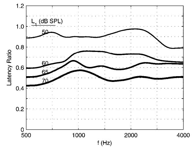
The effect of L₁ on mean SFOAE latency is illustrated by plotting the ratio of the SFOAE latency in each L₁ condition relative to the latency in the L₁=40 dB SPL condition.

E. Group SFOAE SPL results

Although the primary emphasis of this study concerns SFOAE latency effects with level, the measurements also provided group results of how SFOAE SPL varied with L₁. The mean ±1 SE of the SFOAE SPL are plotted in Fig. 11 (gray lines and gray fills, respectively) as a function of L₁. A smoothed-spline approximation using a smoothing parameter p of 0.995 was applied to the mean data to produce a slowly varying estimate of mean SPL (black lines in Fig. 11). The main level effect is that the SFOAE SPL increased compressively with increasing L₁. The SFOAE SPL increased with frequency from 500 up to 1000 Hz, and then decreased with frequency up to 2000 Hz. The SFOAE SPL between 2000 and 4000 Hz was approximately constant for L₁=40-50 dB SPL, and increased with increasing frequency for L₁=60-70 dB SPL.

FIG. 11.

The mean SFOAE SPL are plotted (gray lines) with ±1 SE (gray fills), with increasing line thickness and increasing fill darkness representing increasing L₁ (40, 50, 60, 65, and 70 dB SPL). The smoothed mean SFOAE SPL are plotted as black lines for each L₁, and agree with the unsmoothed SPL to within ±1 SE.

The measurements of SFOAE SPL at each frequency at L₁ ranging from 40 to 70 dB SPL form a SFOAE input/output (I/O) function. The slope of this I/O function was calculated as the change in SFOAE SPL between each pair of adjacent L₁ levels (so that the slope has units of dB/dB), and is plotted versus frequency in Fig. 12. These slopes are parametrized by the higher of the pair of adjacent L₁ levels, namely, at 50, 60, 65, and 70 dB SPL, such that increasing line thickness represents increasing L₁. The four slope curves tend to overlay one another across frequency, except that the slope at the highest level is slightly larger between 600 and 800 Hz and around 4000 Hz. It follows that the slope of the SFOAE I/O function was approximately independent of L₁ up to 65 dB SPL. The SFOAE I/O function slope varied across frequency, with slopes in the range of 0.5-0.6 dB/dB for frequencies from 500 up to 2200 Hz, and larger slopes at higher frequencies reaching 0.75 dB/dB at 4000 Hz.

FIG. 12.

The slope of the SFOAE input-output functions (in dB/dB) are plotted versus frequency. Thicker lines represent responses at increasing L₁ ranging from 50, 60, 65, and 70 dB SPL.

These values are similar to the estimates of compressive growth in Schairer et al. (2003), which ranged from 0.44 to 0.61 dB/dB for frequencies of 1000-4000 Hz. In the Schairer et al. study, a two-slope model of SFOAE I/O function was able to predict the compression and slope of SFOAEs elicited with equal-frequency primaries. This SFOAE model was similar to one used in fitting BM I/O functions (Yates et al., 1990). The SFOAE compression range reported in Schairer et al. (2003) exceeded the slopes of BM I/O functions reported by Yates et al. (1990), and this is also true for the current data. However, it was suggested that some of the difference may be due to the fact that measurements of BM nonlinearity assess forward-transmission effects only, whereas measurements of SFOAE nonlinearity represent forward- and reverse-transmission effects.

IV. DISCUSSION

The main goal of the current study was to examine how SFOAE latency changed as a function of level, and learn what it suggests about changes in dominant SFOAE sources as a function of level. The latency results are addressed in the context of the possible outcomes described in the Introduction (Sec. I C.). Next, the SFOAE latency measurements are used to estimate cochlear tuning.

A. SFOAE sources as a function of stimulus level

The first possible outcome was that SFOAE latencies would be equal at all stimulus levels. However, we found that for any given probe frequency, the SFOAE latency decreased as probe level increased (Figs. 8 and 10). The second possible outcome was that SFOAE latencies in the highest probe-level condition would be near zero. If nonlinear distortion were the dominant source of SFOAEs at the highest probe level, then the latency would be short (near zero) and constant as a function of probe frequency. This was not the case. In the highest probe-level condition, the estimated SFOAE latency was significantly larger than 0 ms and was not constant as a function of frequency (see Figs. 7, 8, and 10).

The experimental results were in accord with the third possible outcome, namely, that SFOAE latencies decreased with increasing stimulus level but remained nonzero. One might expect ear-canal and middle-ear transmission to account for no more than 0.2 ms of round-trip travel time, but the minimum SFOAE latencies were approximately an order of magnitude larger than these travel times, which indicates that SFOAE latencies were dominated by cochlear transmission effects.

These results support the theory that the active process underlying the phase nonlinearity of BM mechanics is also responsible for the nonlinearity in SFOAE latency. SFOAE latencies decreased by approximately 0.5 from the highest stimulus level (70 dB SPL) relative to the lowest (40 dB SPL)(see Fig. 10). The BM group delays reported by Ruggero et al. (1997) decreased by approximately 0.6 from the highest stimulus level (90 dB SPL) relative to the lowest (10 dB SPL). One might expect in any case a greater range of nonlinearity in the non-invasive in vivo SFOAE measurements than in an invasive animal measurement, and there is the additional confounding factor of species differences. The underlying similarity in the level-dependent SFOAE latency results and the nonlinear BM phase measurements suggest that BM nonlinearity is responsible for the observed SFOAE latency effects. Combined measurements of SFOAEs and BM group delay at the tonotopic place in a mammalian cochlea would be useful in further investigating this relationship.

A nonlinear coherent-reflection or other nonlinear-distortion mechanism may also contribute to the response at high stimulus levels, but the results suggest that it is not the dominant source inasmuch as there was substantial latency at all stimulus levels (e.g., Fig. 5).

As described in the Introduction, another mode in which SFOAE latencies might decrease with stimulus level is if the reverse transmission of the SFOAE is via a slower mechanical transmission at low stimulus levels and via a faster acoustical compression-wave transmission at high stimulus levels. The SFOAE latency at low stimulus levels is consistent with the theory of linear coherent reflection (Shera and Guinan, Jr., 2003). Thus, if the compressional-wave mode is involved in SFOAE generation, it would likely be at higher stimulus levels, even though there is no nonlinear theory of SFOAE generation that predicts such a transition between modes of generation. If SFOAE generation is dominated by a compression-wave source, the latency should be approximately equal to the forward transmission time, because reverse transmission via an acoustic compression wave in the cochlear fluid would have a delay that is almost negligible compared to that of forward transmission. In the absence of other nonlinear effects, it follows that SFOAE latencies would be reduced by a factor of one half if an acoustic compressional mode was substituted for the mechanicaltransmission mode. A reduction of latency by one half was observed at high levels in the results of Fig. 10. However, to the extent that the phase nonlinearity of BM mechanics would also reduce SFOAE latency at higher stimulus levels, a reduction by one half due to a dominance of the compression-wave mode would seem likely to reduce the latency by more than a factor of one half. Because such a reduction was not observed, there appears insufficient evidence in the current results to favor the compressional-wave hypothesis, although further research is warranted.

These results are consistent with a coherent-reflection model of SFOAE generation, in which the level-dependent changes in the BM transfer-function phase reduced the SFOAE latency at higher levels. This model of SFOAE generation is assumed in the next section, which uses the measurements of SFOAE latency across frequency and stimulus level to predict effects on cochlear tuning.

B. Using SFOAE latency to estimate Q_ERB

In the current data, the N_SF(f,L₁) satisfied scaling symmetry above 1000 Hz, meaning that at a given stimulus level, the round-trip travel time was a constant number of periods regardless of frequency (above 1000 Hz). Because the assumption of scaling symmetry is met, it follows that SFOAE latency can be used to estimate mechanical resonance bandwidth in cochlear mechanics because bandwidth is related to the forward travel time from the ear canal to the peak place of excitation on the BM (Zweig, 1976; Zweig and Shera, 1995). This forward travel time is N_BM(f,L₁) when measured in units of the number of periods of the stimulus tone. A prediction of the one-dimensional coherent-reflection theory, is that the round-trip SFOAE travel time is twice the forward travel time, so that N_SF(f,L₁)=2×N_BM(f,L₁). Cochlear tuning is quantified in terms of a quality factor Q_ERB, which is defined as the ratio of the stimulus frequency to the equivalent rectangular bandwidth (ERB) of the mechanical resonance on the BM. The roundtrip latency N_SF of SFOAEs elicited by a low-level sinusoid would thus be proportional to Q_ERB. Based on the additional assumption that the best auditory tuning measured behaviorally is constrained by the auditory tuning imposed by cochlear mechanics, the tuning and round-trip latency are related by

$$Q_{\mathrm{ERB}}=k{N}_{\mathrm{BM}}=k{N}_{\mathrm{SF}}∕2,$$ (4)

in which Q_ERB represents either the degree of tuning on the BM or the degree of psychophysical tuning, which can be measured behaviorally using a forward-masking paradigm (Shera et al., 2002). The coefficient of proportionality k is assumed to vary more slowly with frequency than either Q_ERB or N_SF, is known to be similar in the cat and guinea pig, and is assumed to be correspondingly similar in humans.

Using the mean k reported by Shera et al. (k=2.3f^-0.07, where the unit of f is kilohertz), an equivalent Q_ERB(f,L) was calculated as a function of frequency and stimulus level using the measured SFOAE latencies (the effects of the variability in estimating k is outside the scope of the present analyses). The results are shown in the solid-line curves of Fig. 13 in which each curve corresponds to a particular L₁. The SE of N_SF (see Fig. 8) was used to calculate an approximate SE for Q_ERB (at L₁=40 dB SPL), but no additional variability associated with the confidence interval of k was included. Also shown in Fig. 13 are the mean Q_ERB and its 95% confidence interval measured using SFOAE latency (dashed lines; Shera et al., 2002), and the psychophysical values of Q_ERB measured using a forward-masking paradigm with a low-level probe signal in a notched-noise masker (Oxenham and Shera, 2003). These psychophysical data were measured at 1000, 2000, and 4000 Hz, and Q_ERB was calculated using a pair of roex models, shown as individual symbols in Fig. 13. Finally, an alternative set of psychophysical measurements of Q_ERB are shown for the case of simultaneous masking of a probe tone in a notched-noise masker (Glasberg and Moore, 1990). Simultaneous masking is thought to involve suppression and “line-busy” effects at the peripheral level that are not part of forward masking. The present interest is to compare the frequency dependence of these various estimates of auditory tuning, irrespective of the detailed mechanisms underlying each measure of behavioral tuning. Although data are available above 4000 Hz in previous data sets (Oxenham and Shera, 2003; Shera et al., 2002), the data are truncated to the range for which estimates are available for comparison from the current data set.

FIG. 13.

The equivalent Q_ERB (solid lines) derived from the group mean of the SFOAE latencies are plotted with increasing line thickness representing increasing L₁ (40, 50, 60, 65, and 70 dB SPL). The gray fill pattern about the equivalent Q_ERB at L₁=40 dB SPL represents the effect of ±1 SE of the SFOAE latency mean on the estimate of equivalent Q_ERB. The three dashed thin lines show the mean and its 95% confidence interval of the equivalent Q_ERB (Shera et al., 2002) based on SFOAE latencies measured at a stimulus level of 40 dB SPL (also plotted in Fig. 8). The plotting symbols (x and o) at 1000, 2000, and 4000 Hz are psychophysical measurements of Q_ERBbased on a forward masking procedure using a pair of roex models (Oxenham and Shera, 2003). The dashed thick line plots the Q_ERB obtained from simultaneous masking measurements (Glasberg and Moore, 1990).

The simultaneous-masking data support the view that auditory tuning is relatively constant across frequency (Q_ERB≈12), except that the slight reduction to Q_ERB=10 at 500 Hz suggests broader tuning at 500 Hz compared to higher frequencies. The emission-based measurement of Q_ERB by Shera et al. (2002) showed an increase in Q_ERB at higher frequencies, which suggests sharper tuning at 4000 Hz than at 2000 or 1000 Hz. This measurement is directly related to the increase in N_SF at higher frequencies reported by Shera et al. and plotted in Fig. 8. It is notable that the psychophysical measurements of Q_ERB via forward masking (Oxenham and Shera, 2003) are substantially below the confidence limits of their emission-based measurements of Q_ERB at 4000 Hz in Fig. 13; the deviation is in the direction toward the current emission-based estimates of Q_ERB at the L₁ of 40 dB SPL. It is difficult to judge from this plot whether the forward-masking estimates of Q_ERB increase with increasing frequency from 2000 to 4000 Hz, or whether they are independent of frequency. Forward-masking estimates at additional frequencies would be helpful between 1000 and 4000 Hz in understanding the relationship. It should be noted that data in the Oxenham and Shera paper included data points at 6000 and 8000 Hz (not shown), and taken together with the data points shown here, Q_ERB does appear to increase.

While forward-masking experiments at low probe levels show sharper tuning overall than do the simultaneous masking experiments, it is unclear whether their frequency dependence is the same or different. The emission-based estimates of Q_ERB in the current study are relatively constant across frequency from 1000 to 4000 Hz and suggest broader tuning from 500 to 1000 Hz, which is consistent with the simultaneous-masking estimates of Q_ERB. Emission-based estimates of Q_ERB have also been reported at 2700 and 4000 Hz over a similar range of stimulus levels using a pair of transient SFOAE measurement procedures (Konrad-Martin and Keefe, 2005). These results show the expected decrease in N_SF and Q_ERB with increasing stimulus level, but the Q_ERB estimated at the lowest stimulus levels (close to 40 dB SPL) are more similar to the results of Shera et al. (2002) than to the current results. The reasons for the differences between the Konrad-Martin and Keefe and the current results are unknown.

V. CONCLUSIONS

1. SFOAE latency was found to decrease with increasing stimulus level. The low-level measurements of SFOAE latency (at 40 dB SPL) are consistent with the linear coherent reflection theory of SFOAE generation and are inconsistent with the theories of SFOAE generation based on nonlinear distortion or fluid compression. This does not mean that nonlinear distortion and/or fluid compression does not occur at low levels, only that they are not the dominant source, or that their contribution is negligible as measured in the ear canal. The higher-level measurements of SFOAE latency (at 65-70 dB SPL) were approximately half the value of the latency at low levels. The reduction in SFOAE latencies is consistent with previous measurements of BM phase nonlinearity in mammalian cochleae.

2. The SFOAE latency at a given stimulus level is approximately equal to a constant number of stimulus periods between 1000 and 4000 Hz, which supports the prediction of cochlear scaling symmetry, and is slightly reduced between 500 and 1000 Hz. The SFOAE latencies at 40 dB SPL were slightly less between 2000 and 4000 Hz than latencies reported by Shera et al. (2002).

3. The prediction of Zweig and Shera (1995) that SFOAE latency predicts cochlear tuning with a coefficient of proportionality similar to that of other mammals (Shera et al., 2002) was applied to the present data. The results show that cochlear tuning was approximately constant between 1000 and 4000 Hz and slightly broader between 500 and 1000 Hz.

References

- Anderson DJ, Rose JE, Hind JE, Brugge JF. “Temporal position of discharges in single auditory nerve fibers within the cycle of a sine-wave stimulus: Frequency and intensity effects,”. J. Acoust. Soc. Am. 1971;49:1131–1139. doi: 10.1121/1.1912474. [DOI] [PubMed] [Google Scholar]
- Brass D, Kemp DT. “Suppression of stimulus frequency otoacoustic emissions,”. J. Acoust. Soc. Am. 1993;93:920–939. doi: 10.1121/1.405453. [DOI] [PubMed] [Google Scholar]
- Cooper NP, Rhode WS. “Basilar membrane mechanics in the hook region of cat and guinea-pig cochleae: Sharp tuning and nonlinearity in the absence of baseline position shifts,”. Hear. Res. 1992;63:163–190. doi: 10.1016/0378-5955(92)90083-y. [DOI] [PubMed] [Google Scholar]
- Dreisbach LE, Siegel JH, Chen W. “Stimulus-frequency otoacoustic emissions measured at low- and high-frequencies in untrained human subjects,”. Abstracts of the Twenty-First Annual Midwinter Research Meeting of the Association for Research in Otolaryngology; Mt. Royal, NJ. 1998.pp. 349–349. [Google Scholar]
- Glasberg BR, Moore BC. “Derivation of auditory filter shapes from notched-noise data,”. Hear. Res. 1990;47:103–138. doi: 10.1016/0378-5955(90)90170-t. [DOI] [PubMed] [Google Scholar]
- Goodman SS, Withnell RH, Shera CA. “The origin of SFOAE microstructure in the guinea pig,”. Hear. Res. 2003;183:7–17. doi: 10.1016/s0378-5955(03)00193-x. [DOI] [PubMed] [Google Scholar]
- He N,J, Schmiedt RA. “Fine structure of the 2 f1-f2 acoustic distortion product: Changes with primary level,”. J. Acoust. Soc. Am. 1993;94:2659–2669. doi: 10.1121/1.407350. [DOI] [PubMed] [Google Scholar]
- He N, Schmiedt RA. “Fine structure of the 2 f1-f2 acoustic distortion products: effects of primary level and frequency ratios,”. J. Acoust. Soc. Am. 1997;101:3554–3565. doi: 10.1121/1.418316. [DOI] [PubMed] [Google Scholar]
- Kalluri R, Shera CA. “Distortion-product source unmixing: A test of the two-mechanism model for DPOAE generation,”. J. Acoust. Soc. Am. 2001;109:622–637. doi: 10.1121/1.1334597. [DOI] [PubMed] [Google Scholar]
- Keefe DH. “Double-evoked otoacoustic emissions. I. Measurement theory and nonlinear coherence,”. J. Acoust. Soc. Am. 1998;103:3489–3498. doi: 10.1121/1.423058. [DOI] [PubMed] [Google Scholar]
- Knight RD, Kemp DT. “Indications of different distortion product otoacoustic emission mechanisms from a detailed f1, f2 area study,”. J. Acoust. Soc. Am. 2000;107:457–473. doi: 10.1121/1.428351. [DOI] [PubMed] [Google Scholar]
- Konrad-Martin D, Keefe DH. “Transient-evoked stimulusfrequency and distortion-product otoacoustic emissions in normal and impaired ears,”. J. Acoust. Soc. Am. 2005;117:3799–3815. doi: 10.1121/1.1904403. [DOI] [PubMed] [Google Scholar]
- Konrad-Martin D, Keefe DH. “Time-frequency analyses of transient-evoked stimulus-frequency and distortion-product otoacoustic emissions: testing cochlear model predictions,”. J. Acoust. Soc. Am. 2003;114:2021–2043. doi: 10.1121/1.1596170. [DOI] [PubMed] [Google Scholar]
- Liberman MC, Zuo J, Guinan JJ., Jr. “Otoacoustic emissions without somatic motility: can stereocilia mechanics drive the mammalian cochlea?,”. J. Acoust. Soc. Am. 2004;116:1649–1655. doi: 10.1121/1.1775275. [DOI] [PMC free article] [PubMed] [Google Scholar]
- Nuttall AL, Dolan DF. “Two-tone suppression of inner hair cell and basilar membrane responses in the guinea pig,”. J. Acoust. Soc. Am. 1993;93:390–400. doi: 10.1121/1.405619. [DOI] [PubMed] [Google Scholar]
- Oxenham AJ, Shera CA. “Estimates of human cochlear tuning at low levels using forward and simultaneous masking,”. J. Assoc. Res. Otolaryngol. 2003;4:541–554. doi: 10.1007/s10162-002-3058-y. [DOI] [PMC free article] [PubMed] [Google Scholar]
- Ren T. “Reverse propagation of sound in the gerbil cochlea,”. Nat. Neurosci. 2004;7:333–334. doi: 10.1038/nn1216. [DOI] [PubMed] [Google Scholar]
- Ren T, Nuttall AL. “Basilar membrane vibration in the basal turn of the sensitive gerbil cochlea,”. Hear. Res. 2001;151:48–60. doi: 10.1016/s0378-5955(00)00211-2. [DOI] [PubMed] [Google Scholar]
- Rhode WS. “Observations of the vibration of the basilar membrane in squirrel monkeys using the Mossbauer technique,”. J. Acoust. Soc. Am. 1971;49:1218–1231. doi: 10.1121/1.1912485. [DOI] [PubMed] [Google Scholar]
- Rhode WS, Cooper N. “Nonlinear mechanics in the apical turn of the chinchilla cochlea in vivo,”. Aud. Neurosci. 1996;3:101–121. [Google Scholar]
- Rhode WS, Robles L. “Evidence from Mossbauer experiments for nonlinear vibration in the cochlea,”. J. Acoust. Soc. Am. 1974;55:588–596. doi: 10.1121/1.1914569. [DOI] [PubMed] [Google Scholar]
- Ruggero MA, Rich NC, Recio A, Narayan SS, Robles L. “Basilar-membrane responses to tones at the base of the chinchilla cochlea,”. J. Acoust. Soc. Am. 1997;101:2151–2163. doi: 10.1121/1.418265. [DOI] [PMC free article] [PubMed] [Google Scholar]
- Schairer KS, Fitzpatrick D, Keefe DH. “Input-output functions for stimulus-frequency otoacoustic emissions in normal-hearing adult ears,”. J. Acoust. Soc. Am. 2003;114:944–966. doi: 10.1121/1.1592799. [DOI] [PubMed] [Google Scholar]
- Schairer KS, Keefe DH. “Simultaneous recording of stimulus-frequency and distortion-product otoacoustic emission input-output functions in human ears,”. J. Acoust. Soc. Am. 2005;117:818–832. doi: 10.1121/1.1850341. [DOI] [PubMed] [Google Scholar]
- Sellick PM, Patuzzi R, Johnstone BM. “Measurement of basilar membrane motion in the guinea pig using the Mossbauer technique,”. J. Acoust. Soc. Am. 1982;72:131–141. doi: 10.1121/1.387996. [DOI] [PubMed] [Google Scholar]
- Shera CA, Guinan JJ., Jr. “Stimulus-frequency-emission group delay: A test of coherent reflection filtering and a window on cochlear tuning,”. J. Acoust. Soc. Am. 2003;113:2762–2772. doi: 10.1121/1.1557211. [DOI] [PubMed] [Google Scholar]
- Shera CA, Guinan JJ, Jr., Oxenham AJ. “Revised estimates of human cochlear tuning from otoacoustic and behavioral measurements,”. Proc. Natl. Acad. Sci. U.S.A. U.S.A. 2002;99:3318–3323. doi: 10.1073/pnas.032675099. [DOI] [PMC free article] [PubMed] [Google Scholar]
- Shera CA, Tubis A, Talmadge CL. “Coherent reflection in a two-dimensional cochlea: Short-wave versus long-wave scattering in the generation of reflection-source otoacoustic emissions,”. J. Acoust. Soc. Am. 2005;118:287–313. doi: 10.1121/1.1895025. [DOI] [PubMed] [Google Scholar]
- Shera CA, Zweig G. “Order from chaos: Resolving the paradox of periodicity in evoked otoacoustic emissions,”. In: Duifhuis H, Horst JW, van Dijk P, van Netten S,M, editors. Biophysics of Hair Cell Sensory Systems. World Scientific; Singapore: pp. 54–63. [Google Scholar]
- Talmadge CL, Tubis A, Long GR, Piskorski P. “Modeling otoacoustic emission and hearing threshold fine structures,”. J. Acoust. Soc. Am. 1998;104:1517–1543. doi: 10.1121/1.424364. [DOI] [PubMed] [Google Scholar]
- Talmadge CL, Tubis A, Long GR, Tong C. “Modeling the combined effects of basilar membrane nonlinearity and roughness on stimulus frequency otoacoustic emission fine structure,”. J. Acoust. Soc. Am. 2000;108:2911–2932. doi: 10.1121/1.1321012. [DOI] [PubMed] [Google Scholar]
- Tubis A, Talmadge CL, Tong C, Dhar S. “On the relationships between the fixed-f1, fixed-f2, and fixed-ratio phase derivatives of the 2f1-f2 distortion product otoacoustic emission,”. J. Acoust. Soc. Am. 2000;108:1772–1785. doi: 10.1121/1.1310666. [DOI] [PubMed] [Google Scholar]
- Yates GK, Winter IM, Robertson D. “Basilar membrane nonlinearity determines auditory nerve rate-intensity functions and cochlear dynamic range,”. Hear. Res. 1990;45:203–219. doi: 10.1016/0378-5955(90)90121-5. [DOI] [PubMed] [Google Scholar]
- Zweig G. “Basilar membrane motion,”. Cold Spring Harb Symp. Quant Biol. 1976;40:619–633. doi: 10.1101/sqb.1976.040.01.058. [DOI] [PubMed] [Google Scholar]
- Zweig G, Shera CA. “The origin of periodicity in the spectrum of evoked otoacoustic emissions,”. J. Acoust. Soc. Am. 1995;98:2018–2047. doi: 10.1121/1.413320. [DOI] [PubMed] [Google Scholar]
- Zwicker E. “Delayed evoked oto-acoustic emissions and their suppression by Gaussian-shaped pressure impulses,”. Hear. Res. 1983;11:359–371. doi: 10.1016/0378-5955(83)90067-9. [DOI] [PubMed] [Google Scholar]
- Zwicker E, Schloth E. “Interrelation of different oto-acoustic emissions,”. J. Acoust. Soc. Am. 1984;75:1148–1154. doi: 10.1121/1.390763. [DOI] [PubMed] [Google Scholar]