Dynamics of the Neoproterozoic carbon cycle

Abstract

The existence of unusually large fluctuations in the Neoproterozoic (1,000–543 million years ago) carbon-isotopic record implies strong perturbations to the Earth's carbon cycle. To analyze these fluctuations, we examine records of both the isotopic content of carbonate carbon and the fractionation between carbonate and marine organic carbon. Together, these are inconsistent with conventional, steady-state models of the carbon cycle. The records can be well understood, however, as deriving from the nonsteady dynamics of two reactive pools of carbon. The lack of a steady state is traced to an unusually large oceanic reservoir of organic carbon. We suggest that the most significant of the Neoproterozoic negative carbon-isotopic excursions resulted from increased remineralization of this reservoir. The terminal event, at the Proterozoic–Cambrian boundary, signals the final diminution of the reservoir, a process that was likely initiated by evolutionary innovations that increased export of organic matter to the deep sea.

The coevolution of the biosphere and geosphere is reflected in large part by changes in the long-term carbon cycle (1). Past changes within the cycle are recorded in the isotopic content of carbonate and organic carbon buried in ancient sediments (2). Extraordinarily large fluctuations occur in the Neoproterozoic [1,000–543 million years ago (Ma)] carbon-isotopic record both immediately preceding the Cambrian diversification of complex animal life (3–5) and in the ≈200 million years before it (6). There is much interest in determining not only the cause of these isotopic events (3–9) but how, if at all, they are related to early animal evolution (10).

Here we analyze a significant portion of the Neoproterozoic isotopic record by portraying it as a dynamical trajectory in a two-dimensional space indexed by the isotopic content of carbonate carbon and the fractionation between carbonate and marine organic carbon. This depiction, analogous to the construction of phase portraits in dynamical systems theory (11), provides specific predictions for a carbon cycle evolving quasistatically in a succession of steady states. We find that the Cenozoic portion (0–65 Ma) of the carbon-isotopic record satisfies these predictions; however, the Neoproterozoic record does not.

The dynamics of a system with two sizeable and isotopically distinct pools of reactive carbon suffice to explain the Neoproterozoic records. Then as now one pool was oceanic and atmospheric CO₂. Here we show that the other was probably oceanic organic carbon. The isotopic data indicate that this reservoir was large and that its average properties changed slowly. However, fluctuations in its size would have led to major variations in the isotopic record. Moreover, even if the size of the organic reservoir had been perfectly constant, changes in the fractionation associated with organic production would have led to isotopic fluctuations much greater than those predicted by steady-state theory.

The fluctuations of greatest interest are those associated with large-scale glaciations (8, 9) and with the end of the Proterozoic. Large glaciations would have led to enhanced remineralization of marine organic carbon and thus to decreases in the ¹³C content of carbonates. A final diminution of the organic reservoir in the latest Neoproterozoic would have had a similar effect. The terminal event was probably induced by enhanced biomineralization, production of resistant biopolymers, and the invention of fecal pellets by early metazoans, each of which acted to sweep organic carbon from ocean waters.

Each of these conclusions is predicated on our phase-plane analysis, to which we now proceed.

Phase Portraits

We first consider the oceans as a single reservoir of a mass m of carbon, with an incoming flux j_i and an outgoing (burial) flux j_out. The isotopic composition¶ δ of oceanic carbon then changes as (12)

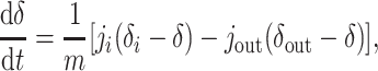[1]

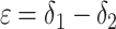
where δ_i is the isotopic composition of incoming carbon, δ_out is the isotopic composition of outgoing carbon in all forms, and m changes according to dm/dt = j_i - j_out. The output occurs as carbonate or organic carbon with isotopic composition δ_a ≃ δ and δ_o = δ_a - ε, respectively. The fractionation ε > 0 results from isotope effects associated with carbonate equilibria and photosynthetic carbon fixation. Assuming that the organic portion of the output is a fraction f [typically ≈0.2–0.3 (13, 14)] of the total, Eq. 1 yields

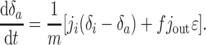[2]

In steady state, j_i = j_out ≡ j^* and the right-hand side above vanishes. Denoting all steady-state quantities with asterisks, we obtain

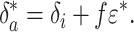[3]

This relation is typically assumed valid at time scales greater than τ = m^*/j^* [≈10⁵ years presently (1, 14)], i.e., for a carbon cycle evolving quasistatically from one steady state to another. In such cases Eq. 3 is commonly used to estimate the organic burial fraction f when δ_a and ε = δ_a - δ_o are known (1, 15). To do so, δ_i is typically set equal to the average isotopic composition of all crustal carbon (1, 15), approximately -5‰ (14).

We consider instead an alternative method for the estimation of f. Specifically we assume only that δ_i and f change more slowly than δ_a and ε, which vary quasistatically such that Eq. 3 holds. Plots of δ_a vs. ε will then describe a straight line whose slope f̂ and intercept δ̂_i are estimates of f and δ_i. In analogy with the theory of dynamical systems, we consider such plots to be phase portraits and seek geometric depictions of dynamical attractors (11). The line described by Eq. 3 is but one (trivial) example, corresponding to a sequence of steady states.

The straight line in Fig. 1a shows that the assumption of quasistatic evolution with constant f and δ_i is reasonable for the Cenozoic. The slope, f̂ ≃ 0.30, and intercept, δ̂_i ≃ -6.1‰, of the line are close to values typical of f and δ_i for the Phanerozoic (13, 14). Fig. 1b displays similar results for the latest Precambrian and early Cambrian, yielding f̂ ≃ 0.29 and δ_i ≃ -8.7‰.

Fig. 1.

(a) The isotopic content of carbonate carbon (δ_a) vs. the fractionation between carbonate and marine organic carbon (ε) for the Cenozoic along with the best-fitting straight line [the reduced major axis (16)]. The slope of the line is f̂ = 0.30, with 95% confidence interval [0.18, 0.36]; its intercept is δ̂_i = -6.1‰ [-7.6‰, -2.8‰] (r = 0.88, n = 12). Confidence intervals are computed by using the bootstrap method (33). (Inset) Time dependence of δ_a (cyan ○) and ε (green □). (b) The same analysis for a more highly resolved period in the latest Precambrian and early Cambrian, resulting in f̂ = 0.29 [0.23, 0.43] and δ̂_i = -8.7‰ [-13.2‰, -7.1‰] (r = 0.96, n = 9). The data, from ref. 15, are computed from global averages. The average standard deviations of these mean values are 0.3‰ (δ_a) and 0.9‰ (ε) in a and 0.1‰ (δ_a) and 0.8‰ (ε) in b.

Fig. 2, however, shows far different results for Neoproterozoic records ranging from ≈738 to 555 Ma. The data in Fig. 2 are displayed four ways, two of which that depend on time (a and b) and two of which that do not (c and d). As shown in Fig. 2 c and d, we find again a straight-line relationship but now with f̂ ≃ 1.0 and δ̂_i ≃ -24‰, values which are extraordinarily high and low, respectively. Of equal interest is the time-ordered depiction of the data in Fig. 2b, where the isotopic excursions are portrayed as a dynamical trajectory in the phase plane defined by ε and δ_a. Except for a brief interlude around 590 Ma, the data lie on a remarkably stable attractor. Fig. 2d, which plots only values of δ_a and ε derived from the same sample (i.e., those for which correlations between strata in different rock units are not required), confirms that the extreme values of f̂ and δ̂_i depend neither on global averaging nor temporal correlation.

Fig. 2.

(a) Time dependence of δ_a (cyan ○) and ε (green □) in the Neoproterozoic computed from global averages (15); the mean standard deviations are 0.6‰ (δ_a) and 1.0‰ (ε). Dotted lines correspond to t = 730, 593, 583, and 555 Ma. (b) Corresponding trajectories in the ε, δ_a phase plane. Arrows indicate the direction of time. Symbols correspond to the following time intervals: ◃, 738–730 Ma; blue •, 730–593 Ma; ⋄, 593–583 Ma; red ▪, 583–555 Ma; ▹, 555–549 Ma. (c) The data from b corresponding only to its blue and red intervals, compared with the best-fitting straight line. The slope f̂ = 0.94 [0.88,0.98] and the intercept δ̂_i = -23.7‰ [-25.0‰, -22.2‰](r = 0.99, n = 28). (d) The complete set of unaveraged ε, δ_a pairs that occur within the same rock sample and contribute to the mean values plotted in c, compared with the best-fitting straight line. The slope f̂ = 0.98 [0.85, 1.15] and the intercept δ̂_i = -24.6‰ [-30.0‰, -20.7‰](r = 0.76, n = 98). Time intervals: blue ○, 731–590 Ma; red □, 583–553 Ma.

The phase portraits of Fig. 2 therefore unambiguously indicate an unusual dynamical state. We next consider its possible causes.

The Neoproterozoic Attractor

How could f̂ ≃ 1.0 and δ̂_i ≃ -24‰? We consider four hypotheses. (i) The Neoproterozoic carbon cycle existed in an extreme state in which inputs and outputs were nearly entirely organic in origin. (ii) Correlations between f and ε or f and δ_i mask less extreme, time-dependent values of f and δ_i. (iii) The results derive from spurious correlations between δ_a and δ_a - δ_o. (iv) The assumption of quasistatic evolution is invalid.

Acceptance of the first hypothesis requires either the virtual absence of carbonate sedimentation or, assuming carbonate deposition rates similar to the Phanerozoic, burial of organic carbon at rates 10-fold those in the Phanerozoic. The former possibility is eliminated by the abundance of carbonates in the Neoproterozoic record (15). The latter possibility requires huge fluxes of organic matter and nutrients and the subsequent deletion of evidence of these processes from the record, presumably by subduction. This combination is highly improbable. Equally fortuitous would be the second hypothesis: Correlations between geochemical variables that conspire to drive f̂ not only upward but all the way to and no further than unity.

The third hypothesis can be rejected quantitatively. If δ_a and δ_o contained no signal but instead were independent random variables with equal variance, plots of δ_a vs. ε = δ_a - δ_o would yield a slope, the reduced major axis (16), of (varδ_a/varε)^1/2 = 1/√2 ≃ 0.71, well outside the 95% confidence intervals for f̂ (see Fig. 2 legend).

The fourth hypothesis, the lack of a steady state, would seem unattractive given that, on average, the data do not resolve time scales less than ≈5 million years, or ≈50 carbon-residence times in the modern oceans (1, 14). Note, however, that f̂ ≃ 1.0 is equivalent to the observation that δ_o ≃ constant, which may be inferred immediately from Fig. 1a or noted directly from figure 1 of ref. 15. If only δ_a responded to contemporary processes whereas δ_o remained invariant due to background recycling of ancient organic material, the data would require the unlikely onset and cessation of that condition simultaneously in multiple sedimentary basins. We therefore seek generic mechanisms that force δ_o to vary slowly while allowing δ_a to change substantially. Slow variation of δ_o implies a large predepositional reservoir of organic carbon that equilibrates slowly with respect to any changes in its inputs or outputs. Provided this equilibration time is slow enough, any such changes will be dynamic rather than quasistatic. The possibility of non-steady-state dynamics therefore deserves further attention.

Theory

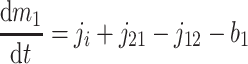
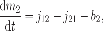
Fig. 3 provides a model. The inventory of carbon in the oceans is partitioned into reservoirs of inorganic and organic carbon, with isotopic compositions δ₁ and δ₂ and residence times τ₁ and τ₂, respectively. The flux from the first to the second reservoir, denoted by j₁₂, represents organic production; it is isotopically depleted relative to δ₁ by an amount ε₀. The return flux, denoted by j₂₁, represents remineralization, with no isotopic fractionation. We identify δ_a = δ₁ and δ_o = δ₂. However, we do not identify ε₀ with ε = δ_a - δ_o. The latter quantity is merely an estimate of ε₀ derived from analyses of buried sediment; only in the case of a steady state will the two be equal in general.

Fig. 3.

A carbon-cycle model with two time scales, τ₁ and τ₂. Reservoir 1 denotes the inorganic carbon of the oceans, with isotopic content δ₁; reservoir 2 denotes organic carbon, with isotopic content δ₂. Fluxes between reservoirs represent photosynthesis (including isotopic depletion by an amount ε₀) and remineralization; fluxes out of the reservoirs represent burial. The flux into reservoir 1 represents volcanic and other inputs with isotopic content δ_i.

The observation that δ_o = δ₂ varies slowly implies that τ₁/τ₂ << 1, meaning that the residence time for organic carbon is much longer than that for inorganic carbon. Variations within the carbon cycle correspond to either changes in the fluxes or changes in the isotopic compositions that the fluxes carry. An example of the former is an increase in the remineralization flux, i.e., an increase in the rate of oxidation of reservoir 2. An example of the latter is a decrease in ε₀ due, e.g., to decreased CO₂ levels or increased algal growth rates (15). An example of both changes is increased erosion of organic-rich strata. If any of these changes occur at a time scale slower than τ₁ but faster than τ₂, δ₁ will decrease while δ₂ remains relatively constant. The difference

[4]

[5]

will almost precisely track δ_a = δ₁, yielding a slope f̂ ≃ 1 in the ε, δ_a phase plane, independent of the real burial fraction f. The resulting line will intercept the δ_a axis at δ̂_i ≃ -24‰ because the steeply sloping trajectories must still pass through the steady solution ε^*, that would occur in the absence of any changes. Slopes f̂ > 1 are also possible. For example, organic production after increased remineralization at time scales somewhat slower than τ₂ would cause δ_o to decrease slowly. Consequently ε = δ_a - δ_o would decrease less than δ_a, yielding f̂ > 1.

These effects can be accompanied by large fluctuations in δ_a. In the case of an increased remineralization flux, the resulting negative excursion is limited only by the change in the remineralization flux itself and in principle could approach δ_o ≃ -24‰. Thus δ_a is not constrained to be greater than δ_i ≃ -5‰, as in steady-state models. Moreover, such large changes need not be accompanied by changes in ε₀, even though ε = δ_a - δ_o will vary with δ_a. However changes in ε₀ are still interesting. In this case δ_a will rise and fall with ε₀. Comparing Eq. 5 with Eq. 3, we see that when such nonsteady changes in δ_a are considered as a function of ε, they are a factor of 1/f ≃ 4 greater than typical (i.e., Phanerozoic) quasistatic fluctuations.

A formal analysis reveals that the dynamic effects can persist at time scales much longer than τ₂. The isotopic compositions and reservoir sizes in Fig. 3 evolve as

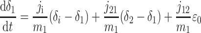[6]

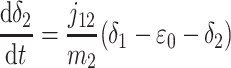[7]

[8]

[9]

where b₁ and b₂ denote burial fluxes for inorganic and organic carbon, respectively, and as in Eq. 1, carbon input to the system is denoted by the flux j_i with isotopic composition δ_i. All fluxes are, in general, time-dependent.

To characterize nonsteady dynamics, we first must obtain the steady solution. The steady state is again given by Eq. 3 but now augmented by relations equating the total input and output fluxes to and from each reservoir. For reservoir 1 we set this flux equal to J₁; i.e., J₁ ≡ j_i + j₂₁ = b₁ + j₁₂. Likewise, for reservoir 2 we have J₂ ≡ b₂ + j₂₁ = j₁₂. We assume that the characteristic residence times in reservoirs 1 and 2 are τ₁ and τ₂, respectively, yielding steady-state reservoir sizes = J₁τ₁ and = J₂τ₂.

Relaxation to the steady state occurs at time scales given by the inverse of the eigenvalues λ₁ and λ₂ of the Jacobian matrix ∂δ̇_j/∂δ_k evaluated at the steady solution:

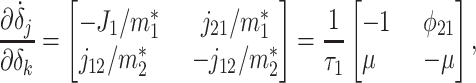[10]

where

[11]

To first order in μ, assuming μ << 1, one finds the eigenvalues

[12]

[13]

The first eigenvalue corresponds to a time scale of order τ₁. However, the slower time scale derived from the second eigenvalue is τ₂/(1 - φ₂₁), which, as φ₂₁ → 1, implies a system-wide relaxation time potentially much longer than τ₂.

Whether the system as a whole will indeed require such a long equilibration time will depend on the particular way in which it is perturbed. Specifically, perturbations parallel to the eigenvector v₁ associated with λ₁ decay like e^λ1t, whereas perturbations with a significant component parallel to the eigenvector v₂ associated with λ₂ decay like e^λ2t. To first order in μ, v₁ ≃ [1, -μ] and . In the limit μ → 0, v₁ corresponds to changes in δ_a but not δ_o, whereas v₂ corresponds to changes in both. Consequently, changes in ε₀, which affect both δ_a and δ_o, will indeed require relaxation times on the order of 1/|λ₂|. However, direct perturbations of δ_a, such as those that result from an enhanced remineralization flux j₂₁, will appear to relax more quickly. In such cases, numerical integrations of the system (Eqs. 6–9), discussed further below, indicate an effective system-wide relaxation time approximately equal to τ₂.

Time Scales and Reservoir Sizes

The various time scales can be estimated. In the modern, preanthropogenic carbon cycle, (1 - φ₂₁) ≃ 10^-2 and τ₁ ≃ 10³ years (14). Accepting these as boundaries, the slowest relaxation time scale in the Neoproterozoic, τ_s ≡ 1/|λ₂|, is

[14]

where the inequality derives from the assumption that μ ≲ 10^-1. The lower bound (14) is conservative: Neoproterozoic CO₂ levels were probably high during nonglacial intervals (1). Combined with other changes, τ_s on the order of 10–100 million years is conceivable.

The evidence for such a long relaxation time lies in the isotopic record. Perturbations to the carbon cycle at time scales much greater than τ_s are quasistatic, simply shifting ε^* and . However, perturbations to δ_a and δ_o at time scales less than τ_s but greater than τ₁ will result in trajectories parallel to the eigenvector v₁. After transformation to the ε, δ_a phase plane, v₁ has slope 1 - μ ≃ 1. Thus the slopes of unity seen in Fig. 2 result from μ << 1, which corresponds to τ₂ = τ₁/μ ≳ 10⁴ years.

In contrast, the average residence time for dissolved and particulate organic carbon (obtained from a mass-weighted sum of inverse residence times) in modern oceans is τ₂ ≃ 40 years (14), yielding μ ≃ 25. Presently j₁₂ ≃ j₂₁ ≃ J₁ ≃ J₂; therefore, m₂ ≃ m₁/μ. Assuming similar relations held in the past and that m₁ has not changed appreciably, we find that organic carbon in Neoproterozoic oceans must have been at least 2–3 orders of magnitude more abundant than at present and that its average age was similarly greater.

Evidently the organic-rich oceans were stratified, with oxygenated shallow waters overlying anoxic deep waters in which organic matter persisted. The redox stratification was maintained dynamically. Before the advent of biomineralization (17) and the evolution of planktonic animals that produced fecal pellets (18), organic material tended to remain in suspension. Any oxygen produced by photosynthesis that had not evaded to the atmosphere would have been consumed by respiration processes in surface waters, with the deep pool of organic matter acting as a buffer against deep-ocean ventilation. [Consequently deep-ocean sulfate concentrations would have also been suppressed (19).] Organic matter that escaped the euphotic zone could have dissolved or aged through fermentative processes, but it otherwise was stored at depth. After upwelling, it could be remineralized, thereby suppressing rises in oxygen concentrations.

Modern oceans provide some supporting evidence. The age of dissolved organic carbon is presently ≈5,000 years (20), which is approximately similar to our lower bound for the Neoproterozoic remineralization time scale, τ₂ ≳ 10⁴ years. Thus Neoproterozoic dissolved organic carbon need not have been extraordinarily old compared with its modern counterpart. However, it was the dominant form, with the result that τ₂ was vastly greater than at present. Studies of Neoproterozoic and older sedimentary organic matter may help to define its chemical form.

Isotopic Events

As already indicated, there are two generic ways to drive the Neoproterozoic isotopic events: by changing the fluxes or changing the isotopic compositions they carry. The latter is exemplified best by variations in ε₀, and we consider it first.

The reality and potential importance of changes in ε₀ are demonstrated by the Cenozoic record. Given the evidence (Fig. 1a) that f was approximately constant and that the carbon cycle evolved through a sequence of steady states, we find ε₀ = ε. The Cenozoic variations in ε therefore must be ascribed to changes in levels of CO₂, abundances of nutrients that controlled rates of algal growth, and aspects of algal physiology such as cell-wall permeabilities and surface-to-volume ratios (21).

All else (i.e., f, reservoir sizes, and fluxes) being constant, changes in ε₀ at a rate ν such that ≲ ν ≲ will generate steeply sloped (f̂ ≃ 1) trajectories provided that μ << 1. We consider the positive excursion seen between 645 and 594 Ma in Fig. 2a as an example. Here ε rises and then falls by ≈5‰. To provide a continuous function plausibly representing related variations in ε₀, we use

[15]

where we set = 28‰, a = 5‰, and ν = (10⁵τ₁)^-1. We then solve Eqs. 6–9 numerically using δ_i = -6‰, specifying a normalized photosynthetic flux φ₁₂ ≡ j₁₂/J₁ = 0.999 and obtaining the normalized remineralization flux φ₂₁ = (φ₁₂ - f)/(1 - f) ≃ 0.999 by choosing f = 0.3. Fig. 4a compares the resulting theoretical trajectory, depicted here through approximately one-half cycle in the variations of ε₀, with observations. The control parameter μ = 10^-2. If τ₁ = 10³ years is assumed, the parameter choices yield τ₂ = 10⁵ years, τ_s ≃ 7 × 10⁷ years, and ε₀ varying with a period of 10⁸ years. The comparison between theory and observations is remarkably good.

Fig. 4.

Neoproterozoic observations compared with theory. (a) The positive excursion between 645 and 594 Ma (blue circles; compare with Fig. 2 a and b) compared with approximately one-half cycle in the evolution of Eqs. 6–9 (smooth green line), with ε₀ varying according to Eq. 15. The control parameter μ = 10^-2. Both trajectories flow in the same clockwise direction. (b) The negative excursion between 583 and 555 Ma (red squares; compare with Fig. a and b) compared with theory (smooth green line), where now ε₀ is constant but the remineralization flux varies according to Eq. 16. Once again μ = 10^-2. Both trajectories flow in the counterclockwise direction.

We next consider changes in fluxes. The large Neoproterozoic organic carbon reservoir suggests an enhanced remineralization flux j₂₁ as a mechanism for driving negative isotopic events. A simple calculation shows how this could happen. Presently the oceans contain ≈3.2 × 10¹⁸ mol of inorganic carbon (14). The Neoproterozoic reservoir of organic carbon should have been at least 10 times greater, i.e., at least 32 × 10¹⁸ mol of organic carbon. Now suppose we seek a 10‰ negative shift in δ_a, from δ_a = 5‰ to δ_a =-5‰, in an inorganic reservoir of modern size. Then if δ_o = -25‰, we need only transfer 1.6 × 10¹⁸ mol of organic carbon, or at most 5% of the organic reservoir, to reservoir 1. Assuming each mole of remineralized organic carbon is oxidized by 1 mol of O₂, such a transfer would require 1.6 × 10¹⁸ mol of O₂. The present-day atmosphere contains ≈37 × 10¹⁸ mol of O₂ (22). Thus only ≈4% of the present atmospheric inventory of oxygen would be required.

As an example, we consider the negative excursion in Fig. 2a between 583 and 555 Ma. We use the same parameter choices as detailed above, but fix ε₀ = and let φ₂₁ vary according to

[16]

for 0 ≤ νt ≤ 1, with equal to the value of φ₂₁ used above, a = 0.23, and ν = 0.03.

Comparison of theory to data is shown in Fig. 4b. If we again assume τ₁ ≃ 10³ years, the time scale of the theoretical trajectory is τ₁/ν ≃ 3 × 10⁴ years. The theoretical and observed trajectories compare well, but the time scales are different. Note, however, that longer time scales are possible: numerical solutions show that the trajectory in Fig. 4b is qualitatively invariant for ν ≃ μ << 1.

Such issues of timing are likely to evolve as the Neoproterozoic time scale itself evolves (23). Although details of our interpretations may change as new absolute dates are obtained, we expect that the overall validity of our model will be insensitive to such revisions.

Discussion and Conclusion

We have deduced the following thus far: (i) the Neoproterozoic carbon cycle evolved dynamically, out of steady state; (ii) the lack of a steady state was due to a large oceanic reservoir of organic carbon; and (iii) the large organic reservoir led to large fluctuations in δ_a either passively, via changes in ε₀, or actively, via temporarily enhanced remineralization. Consideration of pertinent records may well show that the same processes were important at earlier times.

The isotopic records at present cannot distinguish between the passive and active mechanisms. The different senses of rotation in Fig. 4 a and b could help, but remaining geochronological uncertainties and noise in the records probably render inferences statistically insignificant. The fact that changes in ε₀ require longer relaxation times may also be useful, but better estimates of τ₁ and μ and improved geochronology would be required for a definitive conclusion. Isotopic analyses of biomarkers related to photosynthetic pigments, algal sterols, or cyanobacterial hopanoids can indicate variations in the isotopic composition of primary products. These analyses may provide a tool for showing that changes in ε result from changes in ε₀.

Any further interpretation of the isotopic events must of course take into account known environmental changes. Hoffman and Schrag (9) have assembled compelling evidence indicating that apparently fast, deep (≳10‰) declines in the Neoproterozoic δ_a record were accompanied by major glaciations of possibly global extent: a “snowball Earth.” The duration of one or more of these negative excursions may have been as short as 6 × 10⁵ years (24). Such a fast event would be difficult to reconcile with large changes in ε₀. However, it is easily accommodated by a temporary increase in j₂₁. What, then, would have triggered the enhanced oxidation of the organic reservoir?

More O₂ would be partitioned into the ocean in a colder climate. The solubility of O₂ nearly doubles as seawater cools from 30°C to 0°C. Although low temperatures would decrease biological activity, O₂ would be present, and aerobic respiration possible, in a greater portion of the ocean. The effect would be amplified by enhanced convective circulation. Overall rates of remineralization would increase and δ_a would decline.

Concurrent with the decline of δ_a would be an increase in CO₂ levels resulting from the increased oxidation of organic carbon. These changes would have been most significant at low latitudes, where the decrease in temperature due to advancing ice sheets and the surface area over which the change occurred would have been greatest. The attendant atmospheric greenhouse effect then might have acted to arrest the glaciation. The “white-Earth” instability (25) therefore may not have been fully realizable. Glaciations may have advanced near but not entirely to the equator (26).

The terminal Proterozoic negative isotopic excursion (3–5) requires a different interpretation. First, no associations with glaciations have been found (27). Second, its representation in Fig. 1b is consistent with quasistatic rather than dynamic evolution.

The final event is correlated with a dramatic change in isotopic relationships between biomarkers representing primary producers and consumers. That signal has been interpreted as marking the advent of rapidly sinking particulate organic carbon, specifically fecal pellets (18). Although packaging and hydrodynamic factors alone are not insignificant, the requirement that sinking particles include some dense, inorganic ballast is more important (28). Accordingly, the isotopic change may indicate that (i) fecal pellets produced by the first planktonic animals with guts significantly enhanced the combination of organic material with lithogenic debris and/or with calcium carbonate from whitings; (ii) the radiation of algae containing resistant biopolymers in cell walls and cysts (29, 30); or (iii) the development of biomineralization (17).

More broadly, the earlier work postulated linkages between the accelerated removal of organic material from surface waters, the ventilation of ocean depths, and the rise of O₂ (18). To those events is now added the demise of a large reservoir of long-lived organic carbon suspended in seawater. In this view, the ¹³C-enriched secondary biomarkers would have been products of that reservoir and the bacterial processes associated with it. Redox buffering of the deep ocean by sulfide (19) was supplemented by or perhaps even secondary to the effects of the large pool of suspended organic carbon. The interactions inherent in this system lead naturally to the coincidence of three independent isotopic signals: the onset of quasistatic evolution of the carbon-isotopic records (Fig. 1b) and the negative excursion accompanying it (3–5); the disappearance of ¹³C-enriched secondary biomarkers (18); and the onset of complementarity between the isotopic records of carbonate carbon and oceanic sulfate (31, 32). Further correspondences are likely to be found.

References

- 1.Des Marais, D. J. (1997) in Geomicrobiology: Interactions Between Microbes and Minerals, eds. Banfield, J. F & Nealson, K. H. (Mineralogical Society of America, Washington, DC), pp. 429-448.
- 2.Freeman, K. H. (2001) in Stable Isotope Geochemistry, eds. Valley, J. W & Cole, D. R. (Mineralogical Soc. of America, Washington, DC), pp. 589-606.
- 3.Magaritz, M., Holser, W. T. & Kirschvink, J. L. (1986) Nature 320 258-259. [Google Scholar]
- 4.Kimura, H., Matsumoto, R., Kakuwa, Y., Hamdi, B. & Zibaseresht, H. (1997) Earth Planet. Sci. Lett. 147 E1-E7. [Google Scholar]
- 5.Bartley, J. K., Pope, M., Knoll, A. H., Semikhatov, M. A. & Petrov, P. Y. (1998) Geol. Mag. 135 473-494. [DOI] [PubMed] [Google Scholar]
- 6.Knoll, A. H., Hayes, J. M., Kaufman, A. J., Swett, K. & Lambert, I. B. (1986) Nature 321 832-838. [DOI] [PubMed] [Google Scholar]
- 7.Knoll, A. H., Bambach, R. K., Canfield, D. E. & Grotzinger, J. P. (1996) Science 273 452-457. [PubMed] [Google Scholar]
- 8.Hoffman, P. F., Kaufman, A. J., Halverson, G. P. & Schrag, D. P. (1998) Science 281 1342-1346. [DOI] [PubMed] [Google Scholar]
- 9.Hoffman, P. F. & Schrag, D. P. (2002) Terra Nova 14 129-155. [Google Scholar]
- 10.Knoll, A. H. & Carroll, S. B. (1999) Science 284 2129-2137. [DOI] [PubMed] [Google Scholar]
- 11.Bergé, P., Pomeau, Y. & Vidal, C. (1984) Order Within Chaos: Towards a Deterministic Approach to Turbulence (Wiley, New York).
- 12.Kump, L. R. & Arthur, M. A. (1999) Chem. Geol. 161 181-198. [Google Scholar]
- 13.Holland, H. D. (1978) The Chemistry of the Atmosphere and Oceans (Wiley, New York).
- 14.Holser, W. T., Schidlowski, M., Mackenzie, F. T. & Maynard, J. B. (1988) in Chemical Cycles in the Evolution of the Earth, eds. Gregor, C. B., Garrels, R. M., Mackenzie, F. T. & Maynard, J. B. (Wiley, New York), pp. 105-173.
- 15.Hayes, J. M., Strauss, H. & Kaufman, A. J. (1999) Chem. Geol. 161 103-125. [Google Scholar]
- 16.Rayner, J. M. V. (1985) J. Zool. Ser. A 206 415-439. [Google Scholar]
- 17.Lowenstam, H. A. & Weiner, S. (1989) On Biomineralization (Oxford Univ. Press, New York).
- 18.Logan, G. A., Hayes, J. M., Hieshima, G. B. & Summons, R. E. (1995) Nature 376 53-56. [DOI] [PubMed] [Google Scholar]
- 19.Canfield, D. E. (1998) Nature 396 450-453. [Google Scholar]
- 20.Druffel, E. R. M., Williams, P. M., Bauer, J. E. & Ertel, J. R. (1992) J. Geophys. Res. 97 15639-15659. [Google Scholar]
- 21.Popp, B. N., Laws, E. A., Bidigare, R. R., Dore, J. E., Hanson, K. L. & Wakeham, S. G. (1998) Geochim. Cosmochim. Acta 62 69-77. [Google Scholar]
- 22.Keeling, R. F., Najjar, R. P., Bender, M. L. & Tans, P. P. (1993) Global Biogeochem. Cycles 7 37-67. [Google Scholar]
- 23.Walter, M. R., Veevers, J. J., Calver, C. R., Gorjan, P. & Hill, A. C. (2000) Precambrian Res. 100 371-433. [Google Scholar]
- 24.Halverson, G. P., Hoffman, P. F., Schrag, D. P. & Kaufman, A. J. (2002) Geochem. Geophys. Geosyst. 3 10.1029/2001GC000244.
- 25.Budyko, M. I. (1977) Climatic Changes (American Geophysical Union, Washington, DC).
- 26.Hyde, W. T., Crowley, T. J., Baum, S. K. & Peltier, W. R. (2000) Nature 405 425-429. [DOI] [PubMed] [Google Scholar]
- 27.Kaufman, A. J., Knoll, A. H. & Narbonne, G. M. (1997) Proc. Natl. Acad. Sci. USA 94 6600-6605. [DOI] [PMC free article] [PubMed] [Google Scholar]
- 28.Francois, R., Honjo, S., Krishfield, R. & Manganini, S. (2002) Global Biogeochem. Cycles 16 10.1029/2001GB001722.
- 29.Zang, W. L. & Walter, M. R. (1989) Nature 337 642-645. [Google Scholar]
- 30.Derenne, S., Leberre, F., Largeau, C., Hatcher, P., Connan, J. & Raynaud, J. F. (1992) Org. Geochem. 19 345-350. [Google Scholar]
- 31.Veizer, J., Holser, W. T. & Wilgus, C. K. (1980) Geochim. Cosmochim. Acta 444 579-587. [Google Scholar]
- 32.Hayes, J. M., Lambert, I. B. & Strauss, H. (1992) in The Proterozoic Biosphere: A Multidisciplinary Study, eds. Schopf, J. W. & Klein, C. (Cambridge Univ. Press, Cambridge), pp. 129-132.
- 33.Efron, B. & Tibshirani, R. J. (1993) An Introduction to the Bootstrap (Chapman & Hall/CRC, New York).