Dynamics of rat entorhinal cortex layer II and III cells: characteristics of membrane potential resonance at rest predict oscillation properties near threshold

Abstract

Neurones generate intrinsic subthreshold membrane potential oscillations (MPOs) under various physiological and behavioural conditions. These oscillations influence neural responses and coding properties on many levels. On the single-cell level, MPOs modulate the temporal precision of action potentials; they also have a pronounced impact on large-scale cortical activity. Recent studies have described a close association between the MPOs of a given neurone and its electrical resonance properties. Using intracellular sharp microelectrode recordings we examine both dynamical characteristics in layers II and III of the entorhinal cortex (EC). Our data from EC layer II stellate cells show strong membrane potential resonances and oscillations, both in the range of 5–15 Hz. At the resonance maximum, the membrane impedance can be more than twice as large as the input resistance. In EC layer III cells, MPOs could not be elicited, and frequency-resolved impedances decay monotonically with increasing frequency or has only a small peak followed by a subsequent decay. To quantify and compare the resonance and oscillation properties, we use a simple mathematical model that includes stochastic components to capture channel noise. Based on this model we demonstrate that electrical resonance is closely related though not equivalent to the occurrence of sag-potentials and MPOs. MPO frequencies can be predicted from the membrane impedance curve for stellate cells. The model also explains the broad-band nature of the observed MPOs. This underscores the importance of intrinsic noise sources for subthreshold phenomena and rules out a deterministic description of MPOs. In addition, our results show that the two identified cell classes in the superficial EC layers, which are known to target different areas in the hippocampus, also have different preferred frequency ranges and dynamic characteristics. Intrinsic cell properties may thus play a major role for the frequency-dependent information flow in the hippocampal formation.

The storage of information in explicit memory involves both the entorhinal cortex (EC) and the hippocampus (Bannerman et al. 2001; Galani et al. 2002). Rhythmic neural activity plays an important role in this process (Buzsaki, 2002). Oscillations in the theta range (4–10 Hz), often superimposed by gamma rhythms (30–70 Hz), have been observed during explorative behaviour in rats (Chrobak & Buzsaki, 1998). The generation of the theta rhythm is modulated by cholinergic inputs, but may also exploit intrinsic membrane properties. Alonso & Llinas (1989) have reported that near-threshold depolarizations can induce membrane potential oscillations (MPOs) in stellate cells of EC layer II. These cells provide the major input to the dentate gyrus. MPOs have also been observed in the perirhinal cortex (Bilkey & Heinemann, 1999) and deep layers of the entorhinal cortex (Schmitz et al. 1998), and might be transformed into network oscillations through synaptic interactions (Gloveli et al. 1999; Egorov et al. 1999).

MPOs are closely related to resonant behaviour (Lampl & Yarom, 1997; Hutcheon & Yarom, 2000). Resonance properties have been studied by injecting sinusoidal currents with fixed frequencies (Falk & Fatt, 1964; Cole, 1968; Nelson & Lux, 1970; Leung, 1998) or currents whose frequency varies monotonically in time. The latter ‘impedance amplitude profile’ (ZAP) functions allow one to rapidly characterize the resonance properties (Gimbarzevsky et al. 1984; Puil et al. 1986; Hutcheon & Yarom, 2000). Using this method, it has been shown that neocortical neurones (Jansen & Karnup, 1994; Gutfreund et al. 1995; Hutcheon et al. 1996a) and neurones in the trigeminal root ganglion (Puil et al. 1987), mediodorsal thalamus (Puil et al. 1994) and medial geniculate body (Tennigkeit et al. 1997) exhibit an electrical resonance while other neurones act as low-pass filters (Gimbarzevsky et al. 1984). Resonance has also been observed in stellate cells of the entorhinal cortex (Haas & White, 2002), but a systematic study of the resonance properties in entorhinal cortex including a comparison of the main cell classes has not yet been performed. This is, however, of general interest as different cell types within the entorhinal cortex (Van der Linden & Lopes da Silva, 1998) have different targets in the hippocampus. Stellate cells project to the dentate gyrus (Dugladze et al. 2001) while layer III cells project directly to area CA1 (Boulton et al. 1992; Empson et al. 1995). Both cell types have been shown to transfer synaptic inputs in a frequency-dependent manner, with EC layer III cells being most effective at low frequencies (up to 10 Hz) and stellate cells effective at higher (above 5 Hz) frequencies (Gloveli et al. 1997b). We therefore investigated the resonance properties of EC layer II and III cells and their relation to intrinsic subthreshold membrane potential oscillations. Our data analysis is based on a minimal mathematical model which facilitates the qualitative understanding as well as the quantitative comparison of the observed phenomena. This phenomenological description captures the data without any assumption about the intracellular mechanism responsible for the resonance and can thus be applied to any cell type. The model also provides a simple explanation why, contrary to heuristic reasoning, the resonance frequency of a given cell can be larger than its oscillation frequency.

Methods

Brain slices were prepared from adult Wistar rats. All experiments were done in accordance with animal care regulations, recommendations of the European Commission and the Berlin Ethics Committee. The animals were decapitated under deep ether anaesthesia and the brain was removed rapidly from the cranium and placed into cold (4°C) aerated (5% CO₂, 95% O₂) artificial cerebrospinal fluid (aCSF) containing (mm): 129 NaCl, 1.25 NaH₂PO₄, 1.8 MgSO₄, 1.6 CaCl₂, 3 KCl, 21 NaHCO₃ and 10 glucose, at a pH of 7.4. Horizontal slices of the retro-hippocampal region were cut at 400 μm on a vibratome (Vibroslice VSL, World Precision Instruments, Inc., FL, USA) and then transferred to an incubation chamber in which they were stored for at least 1 h at room temperature (∼21°C). Slices for electrophysiological studies were transferred, one at a time, to an interface recording chamber and perfused with aCSF (1.6 ml min⁻¹) at 35°C.

Electrophysiology

Intracellular recordings were obtained using sharp micropipettes filled with 2 m potassium acetate containing 1% biocytin (75–85 MΩ) and an intracellular recording amplifier (Neuro Data model IR-183, New York, USA). All recordings were carried out in current-clamp mode; the series resistance was compensated through bridge balance under visual guidance and verified several times during the recording session; and capacitance transients were removed using the capacitance compensation circuit of the amplifier. The recorded data were low-pass filtered at 3 kHz and digitized by an IO card (DAQCard-AI-16E-4, National Instruments Inc., TX, USA) at a sampling rate of 8 kHz. To block GABA_A, GABA_B and ionotropic glutamate receptors, the following drugs were added in all experiments to the aCSF (μm): 30 6-cyano-7-nitroquinoxaline-2,3-dione (CNQX), 60 dl-2-amino-5-phosphonopentanoic acid (APV), 5 bicucculine (all from Sigma-Aldrich, Deisenhofen, Germany) and 1 CGP55845A: 3-N-[1-(s)-(3,4-dichlorophenyl)-ethyl]amino-2-(s)-hydroxypropyl-P-benzyl-phosphinic acid (CGP), a GABA_B blocker, kind gift from Novartis, Basel, Switzerland).

Stimulus generation

For stimulus generation and data acquisition the program Labview (National Instruments Inc., TX, USA) was used. Hyper- and depolarizing current steps with a duration of 400 and 500 ms were applied to obtain information about the input resistance and general cell properties. To study subthreshold membrane potential oscillations (MPOs), depolarizing currents that lasted for 1 or 10 s were injected such that cells were just below firing threshold.

To obtain impedance amplitude profiles (ZAPs), a frequency-modulated sinusoidal current whose frequency f(t) increased linearly in time (Gimbarzevsky et al. 1984; Puil et al. 1986; Hutcheon & Yarom, 2000) was applied:

with

The time-dependent frequency f(t) of the injected current I(t) was ramped up from f₀ = 0 Hz to the maximum frequency f_m = 20 Hz, as shown in Fig. 1B. The overall duration of the ZAP input current is denoted by T, time by t. The amplitude I_o of the input current was adjusted individually for each cell to reach values of the membrane potential close to firing threshold but not crossing it.

Figure 1. Analysis of membrane potential resonances, as demonstrated by results from a typical EC layer II stellate cell.

A, anatomy and physiology of the sample cell. Main panel: voltage responses to step-current inputs whose size was varied from −420 to 210 pA in steps of 70 pA. The cell displays a pronounced sag potential upon both hyperpolarizing and depolarizing current injections. Left inset: histological reconstruction of the cell. Right inset: amplitude of sag potentials (triangles) in comparison to steady-state voltage responses (circles). B, injected ZAP current (upper panel) and membrane voltage response (lower panel, average from 10 repetitions) as a function of time. Sinusoidal currents with both linearly increasing (shown here) and decreasing oscillation frequency were used. The dashed line in the lower panel indicates the steady-state cell voltage response for a depolarizing step current with the same amplitude as the ZAP current. C, impedance profile of this neurone as determined from the record in B. The arrow at the impedance maximum indicates the resonance frequency, f_res. With 8.9 Hz the resonance frequency falls in the range of 6–15 Hz typical for stellate cells. Inset: phase shift of the voltage response relative to the injected current. At low frequencies the cell shows a small positive phase shift which indicates inductive membrane properties. At higher frequencies, capacitive effects dominate and lead to large negative phase shifts. D, impedance-locus diagram of the same cell. The complex-valued impedance is represented by a vector whose length and angle are shown in the main panel and inset of C, respectively.

The ZAP function should vary rather slowly to obtain a similar precision as when injecting a set of sinusoidal currents. In pilot experiments we tested four different durations for the ZAP function: 5 s, 10 s, 15 s and 40 s. We found that the precision of the measurement improves with increasing T but that it saturates at about 15 s. Accordingly, T was set to 15 s. In five cells we also tested the reversed protocol, where the ZAP frequency changed in the opposite direction, from 20 Hz down to 0 Hz. This modification did not have any measurable effect on the observed resonance phenomena. We can therefore exclude spurious effects due to ionic currents with very slow activation or deactivation. Each ZAP injection was repeated 10 times. Evoked potential fluctuations (Fig. 1B) were averaged over these trials. The subsequent data analyses, curve fittings and simulations were performed using Matlab (MathWorks Inc., Natick, MA, USA). In four cells we also investigated the stability of the resonance properties and repeated the experimental protocol over a long time course (in two cells over 90 min and in two other cells over 180 min). The frequency–impedance relationship was approximately constant over these time intervals.

Histology

After filling the recorded neurones with biocytin, the slices were incubated and stored in 4% paraformaldehyde in 0.1 m phosphate buffer. Shortly before staining, the slices were left in the 30% sucrose solution for 30 min. For staining, the slices were cut at 50 μm on a cryotom (Leika Jung RM 2035, Leitz, Nussloch, Germany). After washing the slices three times in 0.1m phosphate buffer, they were incubated overnight in 0.1 m phosphate buffer containing 1% Triton X-100 (Sigma-Aldrich, Deisenhofen, Germany) and 0.1% avidin Alexa Flour 488 conjuate (AFK, Molecular Probes A-21370, Leijden, the Netherlands). Then the slices were washed again three times with 0.1 m phosphate buffer, mounted on coated object slides, dried overnight at room temperature, dehydrated in 70%, 80% and 96% ethanol and in isopropanol, and glass-covered using 50 ml ProlongAnti-fade Kit (Molecular Probes P-7481, Leijden, the Netherlands) to preserve fluorescent colours. Pictures of stained cells were made using a confocal laser scanning microscope (Leitz, Nussloch, Germany). Cell were identified on the basis of their laminar position and shape.

Analysis of electrical resonance

The frequency-dependent impedance (or ‘transfer function’) was calculated from the ZAP recordings as the ratio between the Fast Fourier Transform (FFT) of the output (measured voltage V) and the input (applied current I):

as shown in Fig. 1 for a typical stellate cell. The impedance contains a real and an imaginary part, Z_real and Z_imaginary. The length of the vector (Z_real, Z_imaginary) measures the amplitude |Z| of the impedance (Fig. 1C and D):

For notational simplicity, |Z| will be referred to as the impedance Z throughout what follows. The angle between the vector and the real axis represents the phase shift between the input current and output voltage (Fig. 1C, inset). Z_real can be interpreted as the resistive component of the cell impedance while Z_imaginary reflects the reactive component. Plotted against each other, the two components form the so-called ‘impedance locus diagram’ (Fig. 1D). Finite sample sizes and possible non-stationarities complicate the precise estimation of the phase shift and impedance at low frequencies. The error is maximal at zero frequency and decreases rapidly with increasing frequency once the duration of the ZAP-input and the number of repetitions are sufficiently large. In our experimental condition the error at 0.5 Hz was about 20%, at 1 Hz about 2% and above 2 Hz less than 1%. For this reason only frequencies above 1 Hz were taken into account.

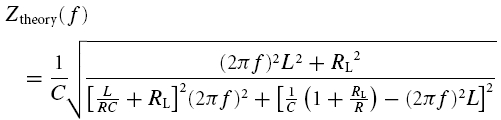
Transfer functions obtained with the ZAP method (eqns (3) and (4)) were fitted with the theoretical impedance–frequency function Z_theory(f) given in eqn (A9), using an iterative algorithm and least-square methods. The phenomenological model (Fig. 2A) underlying the function Z_theory(f) is introduced in the section ‘Mathematical model’, its response properties are discussed in the Appendix. After a satisfactory fit (residual errors vary less than 0.001 per iteration step) was obtained, the model parameters were estimated. To characterize the shape of the impedance profiles, several phenomenological parameters were calculated too (see also Fig. 2B):

• Resonance frequency, f_res: the frequency at which the impedance reaches its maximal value, Z_res. For cells with low-pass properties f_res is set to 0 Hz.

• Sharpness of resonance, Q: the ratio between Z_res and the impedance resulting from a constant current, Z₀. By definition Q is always equal or larger than 1.

• Half-band width, HB: the width of the resonance peak at the height Z_HB = (Z₀ + Z_res)/2.

• High-frequency decay, D: the ratio between Z₂₀, the impedance at the largest tested frequency (20 Hz), and Z₀.

• Half-decay frequency f_HD: the frequency at which the value of the impedance function equals Z_0/2. It characterizes low-pass filter properties of the cell. If f_HD > 20 Hz, this quantity was left as undefined.

Figure 2. Modelling of membrane potential resonances.

A, to quantify the experimental resonance data, a minimal mathematical model was constructed. Its equivalent electrical circuit has two parallel branches. The first branch represents a leaky integrator with resistance R and capacitance C. The second branch models the dynamics characteristic for delayed rectifying currents through a resistance R_L in series with an inductance L. B, schematic drawing of the theoretical impedance profile derived from the electrical circuit model. For each neurone, the model parameters were estimated from least-square fits to the experimental data. In addition, several phenomenological parameters (shown in grey) were calculated to characterize the neurone: resonance frequency f_res, sharpness Q, half-band width HB, high-frequency decay D and half-decay frequency f_HD (see Methods for the precise mathematical definitions).

From a purely mathematical point of view, any Q-value larger than unity indicates a resonance. However, only resonances with sufficiently large Q-values will surpass the intrinsic noise level and thus be of biological relevance. With respect to a functional classification, cells with Q-values between, say, 1.0 and 1.1 can therefore hardly be considered as resonant; on the other hand, resonance curves with Q-values above 1.3 clearly indicate resonant behaviour. As no rigorous functional definition of a ‘best’ boundary value between the two dynamical regimes is possible, we took an intermediate value and considered cells with a Q-value greater than 1.2 as resonant cells. Similarly, cells with a Q-value of less than 1.2 and a D-value of less than 0.8 are referred to as low-pass filters whose attenuation properties are characterized by f_HD if this value can be determined.

Analysis of sag potentials

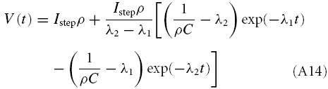
Upon depolarizing or hyperpolarizing current injections a cell might generate a ‘sag potential’, i.e. an overshooting deflection of the membrane potential. From a mathematical point of view, two subtypes can be distinguished (see also Fig. 8 and the Appendix): sag potentials where a damped oscillation with successively decreasing extrema follows the initial deflection (scenario A) and sag potentials with only a single overshoot (scenario B-I). The transition between the two regimes is continuous; due to stochastic components of the intrinsic dynamics, the damped oscillation pattern of scenario A may not even be visible in a recording. To characterize the sag potentials, we fit the appropriate solution of the biophysical model, given by eqn (A13) (scenario A) or eqn (A14) (scenario B-I).

Figure 8. Representation of the response characteristics of the different cell types.

The subthreshold behaviour of a cell can be characterized by two parameters, α and β (see the Appendix for details). Four main classes can be identified for the voltage response to an input current step (boundaries between the regions are represented by the continuous lines): damped oscillations, i.e. sag potentials with multiple decreasing overshoots (A), sag potentials with a single overshoot (B-I), monotonic relaxations (B-II), and unstable solutions (C). The dotted line represents the boundary between formal resonance and non-resonance, where resonance is defined by the mathematical criterion Q > 1. Examples of different response types, based on the minimal mathematical model, are shown on the right panel. The simulations were performed with fixed input impedance and time constant, and thus reflect only the shape of the response, but not the amplitude and actual time course of a biological cell response. Numbers in the main panel indicate the parameter values used for these eight examples. Each data point in the main panel indicates a single measured cell. Stellate cells are represented by circles, pyramidal cells by triangles and non-identified cells by open diamonds. For stellate and pyramidal cells, black symbols show the measurements at resting potential and grey symbols denote measurements above and below resting potential. Data points from the same cell are connected by arrows that point towards increasing membrane potentials. As shown by this representation, the different cell types cluster in parameter space.

Analysis of subthreshold oscillations

Several complementary methods were used to analyse the spectrum and coherence of the MPOs (see Fig. 9 for an example). An analysis based on Windowed Fourier Transforms (WFT) was performed with a running window of length 950 ms and window overlaps of 500 ms using the Welch method (a non-parametric periodogram estimate based on splitting the time series in overlapping segments multiplied by data windows, and on the ensemble average of periodograms computed separately in each data window). Each window was smoothed using a Hanning function to decrease aliasing effects. This method allows one to reduce noise components from the spectrum of Fast Fourier Transform (Lyons, 1998) but introduces an error in the frequency resolution. The WFT is useful for extracting local frequency information, but is rather inaccurate for time–frequency localization, as it imposes a time window and aliases high- and low-frequency components that do not fall within the frequency range of the window.

Figure 9. Membrane potential oscillations (MPOs) of a typical EC layer II stellate cell (the same neurone as depicted in Fig. 1).

A, sample trace of the membrane voltage evoked by a near-threshold depolarizing current injection of 140 pA. B, MPO power spectrum; the spectrum has a pronounced peak at 8.9 Hz. C, auto-correlation function. The dominant frequency is 9.5 Hz, and the small size of the side-peaks indicates a low MPO coherence. D, wavelet spectrum; the dashed contour lines indicate the 95% confidence interval. The time-resolved frequency distribution is characterized by a waxing and waning of the different frequency components and confirms the low MPO coherence. E, time-averaged wavelet spectrum; the dashed line indicates the 95% confidence interval for the global wavelet spectrum. The peak frequency (8.7 Hz) is close to the values obtained in B and C and indicates that the different measures result in similar values. F–H, comparison of the three methods from population data. Except for three cells, the measured values agree well. The dotted straight lines represent the identity where the two respective measures are equal.

To account for a possible non-stationarity of the signal, MPOs were also analysed using a set of orthogonal Morlet wavelets (Torrence & Compo, 1998). This method estimates the correlation of the original signal with a set of sine waves that are modulated by Gaussian filter functions. The analysis allows one to vary the temporal focus of the analysis by changing the width of the wavelet, an advantage over a moving Fourier spectrum. The frequency resolution of the Wavelet analysis is, however, restricted by the number of orthogonal functions.

Power spectra were estimated from both methods using data samples that lasted for 10 s. The peak frequency was taken as a measure for the dominant frequency and the full width at half height was taken as a measure for the coherence of the oscillations. In addition, an auto-correlation analysis was performed to analyse local oscillatory properties. Auto-correlograms (bin width 1.25 ms) were calculated from the same data sets. The time interval between the central and first side peak was used as an estimate for the dominant frequency. The ratio between the magnitudes of the first and second side peaks will be called ‘relative decay’ and served as a further measure for the internal coherence of the oscillations.

The validity and resolution errors of all methods were tested on simulated data traces (sinusoidal 8 Hz oscillations with a duration of 10 s and an amplitude of 2 mV). The frequency estimation from the WFT was 7.99 Hz; the full width at half height was 1.5 Hz. The wavelet analysis led to a frequency estimate of 7.86 Hz, with a full width at half height of 1.6 Hz. The auto-correlation analysis resulted in a frequency of 8.0 Hz and a relative decay of 0.98. All three methods closely coincide with respect to the dominant frequency. While the auto-correlation analysis seemed to be the most precise for the simulated data this method is sensitive to noise in the recorded data and may fail for neurones showing MPOs with low coherence. We therefore always compared the results of all three methods and then computed average values.

Mathematical model

The measured neurophysiological data were analysed within a quantitative framework. We focused on a minimal phenomenological model capable of capturing the essence of the observed neural properties. Using this approach we can precisely determine the differences between the studied cell types, investigate the relation between subthreshold oscillations and resonance phenomena, and make quantitative predictions about responses to time-varying inputs.

The least complicated model accounting for the data is illustrated in Fig. 2A in terms of its equivalent RLC circuit. We chose this intuitive interpretation of the neural dynamics throughout the paper because of its simplicity and direct relation with previous approaches based on the analogy with electrical circuits; see, for example, Koch (1984) or Hutcheon & Yarom (2000). Alternatively, the model can be interpreted as a systematic and linearized reduction of Hodgkin-Huxley type dynamics, as has been shown by various authors; see, for example, Koch (1999) or Richardson et al. (2003).

The model is linear, assumes an isopotential neurone, and consists of two parallel branches. The first branch is characterized by a resistance R in parallel with a capacitance C and mimics the dynamics of a leaky-integrator model neurone. The second branch consists of a resistance R_L in series with an inductance L and endows the model with the general dynamical properties of delayed rectifying currents. The model's effective input resistance ρ is given by ρ = RR_L/(R + R_L).

Note that the parameters R, C, R_L and L are phenomenological parameters that depend on the state (e.g. holding potential) of a neurone. In particular, the capacitance C is an effective quantity that will in general differ from the membrane capacitance (Mauro et al. 1970). It is therefore of particular interest to investigate which parameters change as, for example, the holding potential is varied, and how they change under such variations. These data can help to constrain later detailed biophysical models. In addition, they illustrate the limitations of an overly simplified view that interprets the four parameters as fixed cell properties.

The time evolution of the model is given by two coupled ordinary first-order differential equations:

and

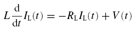where V denotes the membrane potential, as measured relative to the resting potential, and I_L is the current flowing through the inductive branch of the circuit.

This minimal model is deterministic and does not cover the stochastic fluctuations seen in measurements of intrinsic subthreshold oscillations. These fluctuations represent a dynamic balance between damped oscillations of the membrane potential and intrinsic excitations caused by random opening and closing of ionic channels (see, e.g. the review by White et al. 2000). However, such intrinsic noise sources can be easily incorporated into the model. In the spirit of quasi-active neurone models with stochastic components (Steinmetz et al. 2000), we assume that channel noise generates a stochastic intrinsic current I_int(t). Due to the voltage dependence of the channel kinetics, the statistical properties of I_int(t) will in general depend on the mean membrane potential.

The intrinsic current has to be added to the externally applied current I_ext(t) so that the total current I(t) becomes:

It follows from eqn (3) that for vanishing or constant external current, I_ext(t) = I₀, and for any non-zero frequency f, the power spectral densities of the measured membrane potential oscillations V(t) and intrinsic noise currents I_int(t) are related by:

This result is particularly valuable if the membrane potential exhibits a highly irregular time evolution without external stimulation. If, on the other hand, external time-varying currents I_ext(t) are injected into the cell – as is the case for ZAP measurements or step-current inputs – we are mainly interested in the mean, deterministic component of the neural response and may therefore neglect stochastic fluctuations by setting I_int(t) = 0.

The model can be used in these two very different experimental conditions and is thus well suited to quantify salient characteristics of autonomous subthreshold oscillations as well as responses to time-dependent inputs, such as resonance phenomena and sag potentials, within a single mathematical framework.

Statistics

Properties of the identified cells will be characterized by their mean values and standard error of the mean. Resonance and oscillation parameters are given as mean values and standard deviation. Groups were compared using Student's t tests. The significance of a correlation coefficient r was also calculated with Student's t test, t = r(n − 2)^1/2(1 − r²)^−1/2. n is the number of samples. P-values were obtained from standard tables with degree of freedom d = n − 2.

Results

The objective of this study is to characterize the subthreshold behaviour of single EC layer II and III cells and to quantify differences between various cell types. This is done in order to elucidate the role of intrinsic cell properties for the frequency-dependent information flow in the entorhinal cortex and, more generally, the hippocampal formation. Of particular importance are intrinsic oscillations of the membrane potential, responses to time-varying external inputs, and the precise relation between these two different kinds of dynamical single-cell properties.

Membrane potential resonance

Stable recordings were obtained from 67 entorhinal cortex cells in layers II and III. Within this population, 46 cells were identified as stellate cells based on a sag potential occurring both during hyper- and depolarizing current injection, a membrane time constant between 6 and 9 ms, and a resting membrane potential between −58 and −67 mV (Alonso & Klink, 1993; Jones, 1994); 21 of these cells were also morphologically identified as stellate cells (see, for example, Fig. 1A). The cells that were not classified as stellate cells include eight pyramidal cells (see also Fig. 3A) of which five were also morphologically identified. The remaining 13 cells did not show a sag potential and/or had slower membrane time constants and will be referred to as ‘other cells’ (see also Fig. 3B). The data on spike amplitudes, input resistances, resting potentials and time constants are summarized in Table 1. All cells had a membrane potential below −58 mV, an input resistance larger than 20 MΩ and an overshooting action potential.

Figure 3. Impedance profiles of non-stellate cells.

A, example of an EC layer III pyramidal cell with slow spike generation. Shown are voltage responses to step-current inputs whose amplitudes were varied from −490 pA to 140 pA in steps of 70 pA. B, a representative non-stellate ‘other’ cell, located in EC layer II. Depicted are voltage responses to step current pulses (from −350 pA to 70 pA, again in 70 pA steps). C, impedance profile of the cell depicted in A. After reaching a small maximum, the impedance rapidly decreases with increasing frequency: f_res = 2.2 Hz, Q = 1.08, HB = 1.0 Hz, f_HD = 14.0 Hz. Inset: impedance-locus diagram (see Fig. 1D) of the same cell. D, impedance profile of the cell shown in B. The impedance function of this cells also exhibits a small maximum and then decays slowly with increasing frequencies: f_res = 2.5 Hz, Q = 1.03, HB = 1.2 Hz, f_HD = 13.7 Hz. As characteristic for pyramidal and non-stellate cells, the two neurones shown here did not display membrane potential oscillations. Inset: impedance-locus diagram of the same cell.

Table 1.

Measured cell properties

Cell type	Action potential (mV)	Time constant, (ms)	Input resistance (MΩ)	Resting potential (mV)	n
EC-II stellate cells	75.7 ± 5.1	8.5 ± 2.2	32.2 ± 11.2	− 61.5 ± 3.2	46
EC-III pyramidal cells	86.0 ± 8.8	10.9 ± 3.7	56.9 ± 17.4	− 70.4 ± 4.9	8
Other EC cells	83.8 ± 7.9	15.2 ± 1.5	46.2 ± 19.2	− 68.6 ± 4.9	13

Data are presented as means ± s.e.m.

The impedance-amplitude-profile method (ZAP-method) allows one to rapidly characterize neuronal resonance properties (see, for example, Gimbarzevsky et al. 1984; Puil et al. 1986; Hutcheon & Yarom, 2000). When a stellate cell such as that shown in Fig. 1A is stimulated with a frequency-modulated current I_inj(t) as depicted in the upper trace of Fig. 1B, the amplitude of the voltage membrane response first increases as a function of the stimulation frequency, then reaches a maximum before it declines at higher frequencies (Fig. 1B, lower trace).

To quantify the resonance properties of a given cell, the impedance-frequency function Z_theory (eqn (A9)) was fitted to the experimental data. In terms of the model framework (Fig. 2), this provides a compact four-dimensional description (C, L, R and R_L) of the resonance behaviour. Average parameters for different cell classes (at resting membrane potential) are summarized at Table 2. As discussed in Methods and the Appendix, these parameters are phenomenological; in particular, they may depend on the holding potential. For the sample cell of Fig. 1A, the membrane impedance Z is shown in Fig. 1C as a function of the stimulus frequency. The cell has a pronounced resonance (Q = 1.8) at a frequency of 8.9 Hz, with a half-band width HB of 10.0 Hz, and a high-frequency decay D of 1.01 (see Methods for the definition of these quantities). The impedance profile of a characteristic layer III pyramidal cell (Fig. 3A) is shown in Fig. 3C. With a Q-value of 1.08, the resonance of this cell is too weak to surpass the noise level under realistic conditions. For the typical multipolar cell depicted in Fig. 3B, the same is true (Q = 1.03) as evident from Fig. 3D.

Table 2.

Summary of the parameters for equivalent electric circuit

Cell type	R (MΩ)	RL (MΩ)	L (H)	C (μF)
EC-II stellate cells	56.7 ± 17.3	46.1 ± 3.3	1.26 ± 0.11	(3.1 ± 0.2) × 10−4
	(12.2–608.8)	(22.1–92.0)	(0.40–4.0)	((0.2–6.3) × 10−4)
EC-III pyramidal cells	69.9 ± 4.9	34661 ± 11363	173 ± 542	(3.1 ± 0.5) × 10−4
	(59.1–78.8)	(340–59729)	(32–2411)	((2.3–4.7) × 10−4)
EC non-identified cells	26.8 ± 5.0	805 ± 725	6.02 ± 1.8	(6.5 ± 1.6) × 10−4
	(11.6–62.6)	(43–9136)	(0.7–18.5)	((2.1–22.3) × 10−4)

Data are presented as means ± s.e.m. with the range given in parentheses.

Population averages from the measured stellate cells (n = 46) are presented in Fig. 4A. All measurements were done at resting potential unless stated otherwise. As shown by Q-values ranging from 1.2 to 2.1 (Fig. 4B), the impedance at the resonance maximum can be more than twice as large as the input resistance for this cell type. The distribution of resonance frequencies ranges from 6 to 17 Hz with a mean value of 10.6 Hz and a standard deviation of 2.5 Hz. These values suggest that presynaptic inputs oscillating with a frequency of about 10 Hz are most effective in driving this type of neurone. The high-frequency decay D (Fig. 4C) is between 0.53 and 1.44 with a mean of 1.0 ± 0.3. This implies that on average, stellate cells are also integrating high frequency (around 20 Hz) inputs fairly well. The frequency range of the integration region of each individual cell is characterized by its half-band width HB, whose distribution is shown in Fig. 4D. The values range from 6 to 24 Hz with a mean of 11.6 and a standard deviation of 4.3 Hz. This indicates that the region of preferable frequencies is rather wide.

Figure 4. Population data from EC layer II stellate cells (A–D) and EC layer III pyramidal cells (E–H).

A, distribution of resonance frequencies f_res. For the tested stellate cells the distribution has a mean of 10.6 Hz and a variance of 2.5 Hz. This implies that the cells preferentially integrate inputs in the upper theta range. B, distribution of Q-values. With values ranging from 1.2 to 2.1, the maximal impedance is up to twice as large as the input resistance. C, distribution of D-values. The observed values lie between 0.53 and 1.44 with a mean of 1.0 ± 0.3. On average, stellate cells thus integrate inputs with dominant frequencies of about 20 Hz approximately as well as constant inputs. D, distribution of half-band widths HB. The observed values are of the same size or larger than the resonance frequencies and indicate that the resonance curves are rather broad. E, distribution of impedance maximum frequencies f_res for EC layer III cells. For the tested cells the distribution has a mean of 1.1 Hz and a variance of 0.6 Hz. This implies that the cells preferentially integrate inputs at very low frequencies. F, distribution of Q-values. The values range from 1.0 to 1.08 and show that this cell group does not exhibit an impedance resonance. G, distribution of D-values. The observed values lie between 0.17 and 0.49 with a mean of 0.31 ± 0.11. On average, pyramidal cells thus operate as low-pass filters. H, distribution of half-decay frequencies f_HD. The measured neurones show a 50% decay in impedance at frequencies below 20 Hz, and two of the cells even at frequencies around 10 Hz.

These result differ strongly from those observed for EC layer III pyramidal cells. The summary of their resonance properties is shown in Fig. 4E–H. According to our criteria, no cell identified as a layer III pyramidal cell exhibited resonance behaviour. In fact, the highest Q-value observed at rest was 1.2. The resonance profiles of these cells rather resemble a low-pass filter. All cells show at least a 50% decrease in impedance as a frequency of 20 Hz is reached, two cells reach 50% decrease at 10 Hz (Fig. 4H).

Among the other cells, two neurones exhibited a weak resonance with resonance frequencies of 7.4 Hz (Q = 1.28) and 6.0 Hz (Q = 1.23). We also found five cells whose impedance varied only a little between 1 and 20 Hz. Three of these cells displayed membrane potential fluctuations of up to 2 mV but a dominant frequency could not be determined because of very low coherence of the fluctuations. All other cells (n = 11) showed low-pass filter properties with impedance values decreasing at 20 Hz to less than 60% of the value measured by a constant current of the same amplitude. Two of these neurones exhibited a 50% decrease in their impedance already at 10 Hz, five at frequencies below 15 Hz and four other cells at frequencies between 15 and 20 Hz. Some of these cells had a small impedance maximum at frequencies below 3 Hz with Q-values of less than 1.1. A typical example is the multipolar cell of Fig. 3B and D.

Voltage dependence of the electrical resonance and sag potentials

Neural dynamics are governed by voltage-dependent conductances. A more accurate model description of the resonance properties would therefore involve voltage-dependent parameters. The required resonance measurements at different values of the membrane potential are shown in Fig. 5A. These measurements were carried out in seven similar cells at several individually adjusted levels of the membrane potential for each cell, from a slightly hyperpolarized level to the maximum possible subthreshold depolarization. For each resonance measurement, a separate fit to the model (eqn (A1)) was carried out. The changes of the various parameters as the membrane potential was varied are presented in Fig. 5B–F. Definitions of the parameters are given in Method and the Appendix. Surprisingly, both the resonance frequency f_res and the sharpness Q remain almost constant for each investigated cell (Fig. 5B and C). The input resistance ρ and natural frequency f_nat increase slightly upon depolarization (Fig. 5D and E) whereas the decay factor λ decreases (Fig. 5F).

Figure 5. Influence of the holding potential on MPOs and resonance properties of EC layer II stellate cells.

A, determination of the cell impedance at different holding potentials. Left panels: cell responses to ZAP currents of 100 pA with a variable DC component of 100 pA, 0 pA, −100 pA and −200 pA (from top to bottom). Right panels: the corresponding impedance amplitude profiles. B–F, population data from 7 EC layer II stellate cells. Each cell is represented by a different symbol. The cells shown in A is depicted by open diamonds. B, the resonance frequency f_res remains almost constant across the different membrane potentials. C, the sharpness of resonance Q increases slightly upon depolarization. The dashed line indicates the resonance criterium, Q ≥ 1.2, used in this study. D, the input resistance ρ tends to increase upon depolarization. E, the natural freqeuncy f_nat, as predicted by the model with parameters estimated at different levels of membrane potential, remains almost constant upon hyperpolarization and increases slightly upon depolarization, approaching the resonance frequency f_res shown in C. F, the decay factor λ characterizes the exponential decrease of externally triggered oscillations, as estimated from the model, and increases with hyperpolarization and decreases with depolarization. G, sag potentials in response to step-current injections are predicted from the resonance profile. Voltage responses of the cell depicted in A to step-current pulses whose size was varied from −250 to 150 pA in 50 pA steps are shown by continuous lines. Parameters of the model obtained from the impedance resonance curve at the resting potential (A, second row) were used to predict the size and time course of the cell responses (dashed lines). Deviations between model and data indicate non-linear dynamics. For depolarizing currents, the overshooting deflections exceed the theoretical predictions, but the long-term behaviour agrees with the model. For hyperpolarizing current steps, on the other hand, the entire voltage response is scaled-down relative to the model predictions. As discussed in the main text, both phenomena can be explained by an I_h-type current.

According to the biophysical interpretation of the mathematical model, λ should decrease with increasing membrane potential and vanish at the firing threshold. Similar, the natural oscillation frequency f_nat should approach the resonance frequency f_res as the cell is more and more depolarized and become equal to f_res at the firing threshold (see Appendix). Both predictions are in agreement with the experimental data as shown by Fig. 5F and by a comparison of Fig. 5E with Fig. 5B. When the ZAP current was injected at more depolarized membrane potentials action potentials were induced (Fig. 5A, top trace, left panel). Nevertheless the impedance profile which now also reflects the generation of action potentials still shows a peak near the subthreshold resonance peak (Fig. 5A, right panels).

The frequency f(t) of the ZAP-function input (eqn (2)) increases linearly in time (eqn (3)) so that equal frequency bandwidths are covered in equal time intervals. Taking advantage of this property, we quantified the suprathreshold neural response within four adjacent frequency bands, each with a width of 5 Hz. The cell shown in Fig. 5A generated a total of 229 spikes in the 10 trials: 14 (6.1%) in the frequency range from 0 to 5 Hz, 115 (50.2%) in the 5–10 Hz range, 96 (42.0%) in the 10–15 Hz range, and 4 (1.7%) in the 15–20 Hz range. Across all investigated stellate cells these ratios were: 3.3%, 48.1%, 43% and 5.6% for the four frequency bands, respectively. Notably the cell with a resonance frequency around 17 Hz (shown by the plus marks in Fig. 5B–E) did not spike at all at frequencies below 5 Hz and produced 13.0%, 45.1% and 41.9% spikes in the remaining three consecutive frequency bands. Together these findings suggest a close relation between the subthreshold properties and the suprathreshold firing characteristics.

Evidently, a minimal isopotential model that is based on parameters obtained at one single level of the membrane potential cannot fully describe the entire neural subthreshold behaviour, e.g. sag potentials (Van der Linden & Lopes da Silva, 1998). Nevertheless, we tried to predict their size and time course, based on model parameters obtained at the level of resting membrane potential, as shown in Fig. 5G. As the model is linear without voltage-dependent dynamics, deviations of the measured sag potentials from the model predictions are therefore clear indicators for such dynamics.

Close inspection of Fig. 5G reveals that for depolarizing step currents, the overshooting transients are indeed larger than the theoretical predictions, although the cell's long-term behaviour is in excellent agreement with the model at all tested depolarization levels. For hyperpolarizing step currents, on the other hand, the entire voltage response confirms the model predictions apart from an overall scaling factor. These findings imply that currents with different dynamics are activated depending on the level of the membrane potential. In the hyperpolarized regime, the observed phenomena can be explained by a rapidly activated and long-lasting current. Such dynamics have been reported for the I_h current (see, for example, Dickson et al. 2000a). In the depolarized regime, however, the voltage-dependent conductance quickly inactivates after the initial transient. This may be explained by a de-activation of the hypothetical I_h current or an activation of a slow delayed-rectifier potassium current, such as I_KS, I_M, or I_D. All these currents have been previously described in stellate cells (Eder et al. 1991; White et al. 1993; Eder & Heinemann, 1994, 1996; Richter et al. 2000; Shalinsky et al. 2002).

The filter characteristics of layer III pyramidal cells remained about the same when the membrane potential was varied, similar to the situation in stellate cells (Fig. 6). The input resistance of the pyramidal cells increased with increasing membrane potential (Fig. 6D), again in accordance with the results from stellate cells (Fig. 5C). Upon supra-threshold depolarization the cell of Fig. 6A fired predominantly at frequencies around the modest maximum of the resonance profile. The cell shown in Fig. 6A produced 9–15 spikes in each of the 10 repetitions, and a total of 131 spikes: 94 (71.8%) in the frequency range between 0 and 5 Hz and 37 (28.2%) in the 5–10 Hz range. Across all investigated cells this ratio was 86.3%, and 13.7% for these two frequency bands. Notably, none of the investigated cells spiked when presented with ZAP frequencies above 10 Hz. Thus, as for stellate cells, subthreshold properties strongly influence the firing pattern above but close to the firing threshold.

Figure 6. Influence of the holding potential on membrane potential resonances of EC layer III pyramidal cells.

A, left panels: voltage responses of a typical EC layer III pyramidal cell to ZAP-current inputs with an amplitude of 100 pA and a DC level of 200 pA, 100 pA, 0 pA, and −100 pA (from top to bottom). Right panels: the corresponding impedance profiles. B–D, data from three EC layer III pyramidal cells. Each cell is represented by a different symbol. The example shown in A is depicted by open diamonds. B, the location of the impedance maximum f_res remains approximately constant across the different membrane potentials. C, apart from the two supra-threshold responses, Q-values are always below the resonance criterion Q ≥ 1.2. The investigated cells thus do not show resonance at subthreshold membrane potentials. D, as for stellate cells (see Fig. 5C), the input resistance ρ increases with depolarization.

Interestingly, for all investigated cell types, resonance frequencies can be predicted with high accuracy using just the product of two cell parameters, the capacitance C and inductance L (Fig. 7A), whereas the two resistances R and R_L play only a minor role. Furthermore, the half-band width HB is roughly equal to the resonance frequency f_res (Fig. 7B), at least in the frequency range between 0 and 10 Hz. At higher resonance frequencies, HB increases super-linearly. A positive correlation between resonance frequency and half-band width is to be expected from the model. Consider, for example, the effects of changing the inductance L. Larger L-values imply longer effective delays of the rectifying current and thus a more pronounced resonance – higher Q and smaller HB values. At the same time, increasing L (and thus decreasing the resonance frequency of the ideal resonator) decreases f_res (Fig. 7A). Together, these two effects cause the half-band width to correlate positively with the resonance frequency (Fig. 7B).

Figure 7. Generic properties of the impedance function in EC neurones.

A, relation between the measured resonance frequency and the frequency of an ideal resonator (R = R_L = 0) with the same capacitance and inductance. The measured data form a continuum and cluster in the vicinity of the main diagonal. Accordingly, resonance frequencies are well predicted by the values of the elements C and L of the equivalent electrical circuit. B, relation between the resonance width HB and the location f_res of the impedance maximum. At least for small frequencies, both quantities are almost identical. C, sample-averaged impedance profiles for the two main investigated cell classes. EC layer III pyramidal cells have low-pass filter properties, whereas EC layer II stellate cells exhibit pronounced resonance phenomena.

As has been pointed by Hutcheon & Yarom (2000), resonance phenomena are closely related to membrane potential oscillations, and manifest themselves not only in the responses to oscillatory input but also in the responses to step-current inputs. Following Richardson et al. (2003), we defined two parameters, α and β (see Appendix), that allow one to characterize the neural responses within a two-dimensional graphical representation (Fig. 8). Based on the model framework, damped oscillations are expected in a certain parameter region, which we call region A (see Appendix and Fig. 8). Sag potentials should exist in region A (multiple overshoots) as well as in region B-I (single overshoots); see eqns (A13) and (A14), respectively. Cells that fall into region B-II should not exhibit sag potentials but rather approach the new holding potential in a monotone fashion. Transitions between the expected phenomena in the different regimes are smooth, as also demonstrated by the schematic examples in the right panels of Fig. 8. Furthermore, secondary and subsequent overshoots (in parameter regime A) may hardly be visible in recorded data as the oscillation amplitude rapidly decreases for realistic values of the decay factor λ. Finally, it is important to realize that the boundary between the domain where sag potentials occur (regions A and B-I) and where no sag potentials occur (B-II), does not coincide with the curve that separates band-pass behaviour (Q > 1, above the dashed line in Fig. 8) from low-pass behaviour (Q = 1, below the dashed line) in resonance experiments, cf. eqn (A21).

To test how these predictions relate to the observed data, the parameters α and β (eqns (A15) and (A16)) were calculated for all neurones from the resonance experiments. Putting each cell at its proper position in the α/β-plane (Fig. 8) demonstrates that the different cell classes cluster in different regions of this plane. All stellate cells (filled circles) fall into region A, and far from the boundary with region B-II. Based on data from the resonance experiment only, the model thus predicts that stellate cells exhibit prominent sag potentials, as indeed observed (Fig. 4B).

All but one EC layer III pyramidal cell are below or very near the dashed line, in accordance with Fig. 4G. Some of these cells do fall into region A, but close to the boundary with region B-II. The expected weak sag potentials were not observed. This can be attributed to the difficulty of clearly identifying sag potentials from voltage traces in this transition zone. The remaining ‘other cells’ did show weak sag potentials, again as predicted by the model.

Membrane potential oscillations

Upon depolarizing current injection to membrane potential values near the firing threshold, spontaneous membrane potential oscillations (MPOs) were displayed by all stellate cells tested for this behaviour. In preliminary experiments we had found that the generation of an action potential generally resulted in subsequent MPOs with larger amplitudes than those evoked after depolarization that do not cause action potentials. To avoid any spurious effects our data analysis is therefore exclusively based on recordings that did not contain any action potentials.

Typical MPOs are depicted in Fig. 9A. They were generated by the sample stellate cell of Fig. 1A in response to a constant depolarizing current injection of 140 pA. A characteristic feature of the observed subthreshold activity is its irregularity compared to an ideal periodic oscillation. This is also evident from the power spectral analysis which generally resulted in broad frequency distributions. For the particular cell shown in Fig. 9A, the peak frequency is 8.9 Hz (Fig. 9B). The full width at half-maximum is 3.5 Hz (from 7.4 to 10.9 Hz). An auto-correlation analysis (Fig. 9C) provides information on both the dominant frequency and the coherence of the oscillations. In this particular cell, the dominant frequency is 9.5 Hz, close to the value obtained with the power spectral analysis. The coherence of the MPOs, defined as the ratio of the second to the first side peak in the auto-correlation function, is 0.22. This ather low value is in accordance with the cell's power spectrum and typical for the whole cell population (data not shown). A wavelet analysis (Fig. 9D) reveals the time-resolved frequency distribution of the membrane potential fluctuations. The time course is characterized by a waxing and waning of different frequency components within the MPOs, in agreement with the low MPO coherence of this cell. The temporal average of the wavelet spectrum from Fig. 9D is depicted in Fig. 9E. Its peak frequency of 8.7 Hz is close to the values obtained from the power spectrum and auto-correlation analysis. To reduce spurious effects due to possible artefacts of each individual method, oscillation frequencies f_osc were always determined as the average obtained from the three methods. For all but three cells the three different measures agree well (Fig. 9F–H) so that we may use average values to reduce potential numerical artifacts. A summary of the oscillation frequencies f_osc from all analysed stellate cells (n = 30) is shown in the inset of Fig. 10. The distribution of measured f_osc values extends from 3 to 14 Hz with a mean value of 9.0 Hz and a standard deviation of 2.2 Hz.

Figure 10. Resonance and MPO frequencies in EC layer II stellate cells.

The relation between oscillation f_osc and resonance f_res frequencies for the all investigated EC layer II stellate cells is shown. In every measured cell the MPO frequency (obtained as averages from the power spectrum, auto-correlation function and wavelet analysis) is lower than the resonance frequency. Both quantities are strongly correlated. Inset: population histograms for both oscillation (filled bars) and resonance (open bars) frequencies.

As demonstrated by these results, intrinsic subthreshold activity in the investigated stellate cells is characterized by oscillations with a pronounced peak in the power spectrum but low temporal coherence. The shape of the power spectrum and, in particular, the location of its maximum are reminiscent of membrane impedance curves – cf. Figs 9B and 1C. To examine this relationship, we compared f_osc with f_res (Fig. 10) for all investigated cells. Our data indicate that the resonance frequencies f_res are always higher than the MPO frequencies f_osc. In addition, there was a strong correlation between both frequencies (r = 0.83, t = 7.27, d = 28, P < 0.001).

Within the model framework, these findings are readily explained. According to eqn (8), the power spectrum of the observed MPOs is equal to the product of the intrinsic noise power spectrum and the squared impedance profile. This profile is known from the resonance experiments (Fig. 1C). We did not attempt to measure the detailed frequency dependence of the noise spectrum as we were primarily interested in the relative positions of the maxima of |V|(f) and |Z|(f). However, it is well known that channel noise generates a rather smooth spectrum that gradually falls off with increasing frequency f (Hille, 1992; White et al. 1998). Equation (8) then predicts that f_osc, i.e. the frequency at which |V|(f) has its maximum, is smaller than f_res, i.e. the frequency at which |Z|(f) has its maximum. This prediction is in full agreement with the measured data for every single neurone (Fig. 10). The difference between f_res and f_osc varies from cell to cell, which may be due to slight variations of the intrinsic noise spectrum. Care should be taken, however: membrane potential oscillations were measured near threshold whereas the resonance profiles were derived from data close to the resting potential. Thus |V|(f) and |Z|(f) correspond to different neural states. However, as shown in Fig. 5B, the resonance frequency is almost independent of the membrane potential so that f_res and f_osc may, indeed, be directly compared.

Let us finally turn to the oscillatory properties of non-stellate neurones: pyramidal cells did not exhibit MPOs, as described earlier for layer III projection cells by Gloveli et al. (1997a, 1999) and Van der Linden & Lopes da Silva (1998). We also found five ‘other’ cells whose impedance varied only a little between 1 and 20 Hz, and three of these cells displayed fluctuations of membrane potential of up to 2 mV. However, a dominant frequency could not be determined reliably because of very low coherence of the membrane potential fluctuations. Therefore, within the studied cell classes, pronounced membrane potential oscillations seem to be a characteristic feature of stellate cells.

Discussion

Our findings about the intrinsic dynamics of different neurones within the superficial layers of the entorhinal cortex can be summarized as follows: EC layer II stellate cells exhibit both a prominent peak of their frequency-resolved membrane impedance and noise-driven subthreshold membrane potential oscillations in the upper theta frequency range. Contrary to this situation, non-oscillatory EC layer III cells (pyramidal neurones and ‘other cells’) have at most a small impedance maximum at a frequency below the theta range or display only pure low-pass filter characteristics. In accordance with the theoretical predictions, all resonant cells react with a prominent sag potential upon both depolarizing and hyperpolarizing current injections and all oscillatory cells exhibit resonance. The frequency of near-threshold MPOs in stellate cells is similar but always lower than their resonance frequency, measured at the resting potential. Extending and complementing previous findings, these data suggest that different cell types in the entorhinal cortex vary significantly with respect to their integrative properties in the temporal domain. As EC layer II stellate cells provide the major input to the dentate gyrus while EC layer III pyramidal cells mainly project directly to area CA1, our results also suggest that time-structured information is transmitted in a differential and frequency selective way to different down-stream regions of the hippocampal formation.

Membrane potential oscillations

Previously, MPOs had been reported for stellate cells of layer II of the entorhinal cortex (Alonso & Llinas, 1989; Van der Linden & Lopes da Silva, 1998; Dickson et al. 1997, 2000a), for deep-layer projection cells of the entorhinal cortex (Schmitz et al. 1998; Dugladze et al. 2001; Gloveli et al. 2001) and for cells of the perirhinal cortex (Bilkey & Heinemann, 1999). Oscillatory properties of CA1 pyramidal cells have also been observed upon depolarization to values very close to or above firing threshold (Buhl et al. 1996; Pike et al. 2000). In addition, many cortical pyramidal cells display membrane potential oscillations when depolarized or exposed to carbachol (Metherate et al. 1992; Amitai, 1994). Frequencies range from 4 to 16 Hz and can thus be classified as theta activity according to the rodent literature (for a review see, for example, Gottesmann, 1992a,b). It has also been suggested that such MPOs are involved in the generation of network oscillations in the same frequency range (Alonso & Llinas, 1989). Conductance-based models suggest that MPOs can depend on a variety of ionic currents determined by the cell type (Wang, 1993; Desmaisons et al. 1999). MPOs in stellate cells have been analysed by Dickson et al. (2000a,b). The model proposed by these authors suggests that the interplay between a persistent sodium current and a hyperpolarization-activated cationic current (I_h) is responsible for the observed MPOs. Within the authors' deterministic framework, MPOs are then interpreted as limit-cycle oscillations of a non-linear dynamical system. Based on the observation of highly regular MPOs in systems such as the inferior olive, this view has also been put forward by various other authors (see, e.g. Lampl & Yarom, 1997; Hutcheon & Yarom, 2000).

In accordance with previous investigations (White et al. 1998, 2000), the irregularity and low coherence of the subthreshold oscillations observed in our study requires a different explanation and suggests that intrinsic noise sources play a paramount role for the generation of MPOs in the entorhinal cortex. This precludes the use of deterministic models to describe MPOs and alters their mechanistic interpretation. In fact, our data indicate that MPOs are not caused by an instability of the equilibrium state of a low-dimensional deterministic system but rather by stochastic forces that are most likely to be due to channel noise. Thus although the same or similar ionic currents may be involved as in the picture of Lampl & Yarom (1997), Dickson et al. (2000a,b) or Hutcheon & Yarom (2000), these currents do not cause deterministic periodic oscillations but exhibit stochastic fluctuations. The striking difference between the entorhinal cortex and inferior olive may partly be due to the self-entrainment caused by electric couplings in the inferior olive.

The primary physiological function of intrinsic membrane potential oscillations might be an augmentation of synaptic inputs that are in synchrony with ongoing MPOs (Volgushev et al. 1998). This is particularly important when cells are depolarized for prolonged periods of time to membrane potentials near their firing threshold, for example during cholinergic input. But intrinsic oscillations may also support network oscillations, particularly if mechanisms exist which synchronize the individual MPOs in neural ensembles. This could be accomplished by a phase-resetting mechanism, for example by synchronous inhibitory synaptic input to a group of cells or by electrical coupling between those cells. In our histological preparations we rarely observed dye coupling between stellate cells; a more focused study would be required to identify mechanisms by which MPOs could be synchronized. By interaction with interneurones, MPOs in a given set of cells might also be translated into superimposed higher frequencies, as suggested by findings of Gloveli et al. (1999). In this study, carbachol application to deep layer cells in the EC induced rhythmic synaptic potentials in superficial entorhinal cortex cells containing both theta and gamma frequencies.

Resonance properties

In many early studies of single-neurone properties only stationary input resistances were determined. However, once researchers started to expose cells to oscillating current injections it became evident that the cell impedance may strongly depend on the stimulation frequency (Falk & Fatt, 1964; Cole, 1968; Mauro et al. 1970; Nelson & Lux, 1970). A number of cell types in the mediodorsal thalamus (Puil et al. 1994), the inferior olive (Lampl & Yarom, 1997) or the entorhinal cortex (Haas & White, 2002) were found to display resonant properties. With improved understanding of the underlying cellular physiology, it was then realized that MPOs and neural resonance are closely related phenomena, as reviewed by Hutcheon & Yarom (2000).

As shown by our study, MPOs do occur in neurones that are intrinsically resonant while resonance itself is not sufficient for MPO generation. This finding implies that one has to carefully distinguish between the conditions under which neurones exhibit resonance and those for subthreshold oscillations; even in an intrinsically resonant cell MPOs are simply not possible if the intrinsic noise level is so low that there are not enough ionic current sources to trigger measurable voltage fluctuations. Together with the irregular nature of MPOs, these findings underscore the importance of stochastic descriptions of subthreshold phenomena (for a review, see White et al. 2000). As demonstrated by our modelling results, a simple two-dimensional linear model can account quantitatively for the observed phenomena.

The cell classes investigated in this study differ widely in their resonance behaviour. Stellate cells from layer II of the entorhinal cortex possess a resonance with an impedance increase between 20% and more than 100% at the resonance frequency while for other cell types the impedance function either has only a small peak or simply decays with increasing frequency. Pyramidal neurones of EC layer III exhibit clear low-pass filter properties and thus differ significantly from the stellate cell population (t = 7.6, d = 41, P < 0.001). The cut-off frequency of the low-pass filter was always less than 5 Hz with a half-decay frequency of less than 20 Hz. This implies that EC layer III pyramidal cells integrate synaptic input best for frequencies below 5 Hz while stellate cells integrate input best in the frequency range from 5 to 15 Hz. Note also that our heuristic resonance criterion (Q ≥ 1.2) nicely reflects the dichotomy seen in the population data (cf. Fig. 3B and G).

The frequency-dependent information transfer between two neurones can be strongly influenced by the synaptic properties of the presynaptic cell (see, e.g. Markram et al. 1997). As demonstrated by the large differences of the resonance properties of EC layer III pyramidal cells and EC layer II stellate cells, respectively, the integrative properties of the postsynaptic cell may be an equally important factor.

In the current study we did not make an attempt to identify ionic currents responsible for the resonance behaviour through pharmacological methods. Possible candidates for these currents are slowly activated currents that oppose changes of the membrane voltage. In CA1 pyramidal neurones two different resonance currents (I_M and I_H) have been identified as acting upon depolarization and hyperpolarization (Hu et al. 2002). Those currents have also been identified in stellate cells. Simulations have shown that a model that includes I_M, I_H and I_Nap in addition to the classical Hodgkin-Huxley currents I_Na, I_K and I_L (Hodgkin & Huxley, 1952) provides a good description of the observed resonance characteristic for an average stellate cell. Nevertheless, the other voltage-dependent currents observed in stellate cells (Eder et al. 1991; White et al. 1993; Eder & Heinemann, 1994, 1996; Bruehl & Wadman, 1999; Magistretti & Alonso, 1999; Richter et al. 2000; Shalinsky et al. 2002) may also play a role in precisely tuning the cell frequency profile and may also help to explain the large variability of the individual cell frequency preferences. As ion channels may be differentially distributed on dendritic and other cellular compartments, differences in resonance properties are expected not only between individual cells but also between structural regions within the same cell. Indeed, when comparing dendritic and somatic recordings of cortical pyramidal cells, significant differences in resonance behaviour were observed by Ulrich (2002).

We have found a number of EC cells whose impedance was approximately constant over the whole investigated frequency range. We have not identified these ‘other’ cells. It could be that they are GABAergic cells. Furthermore, we cannot exclude the possibility that some of the recordings may have resulted from measurements in dendrites.

From single-cell to network oscillations

Average impedance profiles for the two identified cell groups are depicted in Fig. 7C. On average, EC layer III pyramidal cells integrate low-frequency inputs best in the range below 5 Hz, while stellate cells are more responsive to inputs at higher frequencies. When we applied a ZAP input at strongly depolarized membrane potentials, action potentials were generated at the frequencies close to the resonance frequency. This is in agreement with previous studies on frequency preferences in the entorhinal cortex. For example, during repetitive synaptic subthreshold stimulation with frequencies below 5 Hz, the pathway from the EC layer II to the dentate gyrus remains quiet and is preferentially activated with frequencies above 5 Hz (Gloveli et al. 1997b). In contrast, EC layer III cells projecting to the subiculum and CA1 area respond preferentially to low stimulus frequencies (below 10 Hz) and are strongly inhibited when stimulated with higher frequencies (Heinemann et al. 2000). Both cell classes possess a common range of frequencies between 5 and 10 Hz where integration of synaptic inputs is similarly effective. It would be interesting to investigate how this finding is related to the ease of theta-rhythm induction in the hippocampal formation and to study the implications of impedance resonance for synaptic plasticity.

Appendix

In what follows, we derive basic properties of the deterministic model used to analyse mean neural responses when time-varying external inputs are applied to a neurone. We then discuss the model predictions for fitting data obtained from experiments with oscillatory and step-current inputs. Most of the results can also be found in previous publications (see, e.g. Puil et al. 1986; Hutcheon et al. 1996a; Richardson et al. 2003). We therefore do not provide an in-depth derivation but rather present the various results using one unified nomenclature. The stochastic extension of the model is described in the Results section.

Stability of steady state solutions and natural oscillation frequency

We analyse the membrane potential dynamics within the RLC-circuit framework described by eqns (5) and (6). Here, C, R, L and R_L are phenomenological quantities that may change their value as the holding potential is varied. By definition, the effective cell capacitance C is always positive. However, the other parameters could, in principle, change their sign. As we will see shortly, certain parameter combinations have to do so when the membrane potential of the model cell looses stability – which corresponds to the firing threshold in a real neurone.

We first analyse the conditions under which stable steady state solutions (i.e. stable resting potentials) are possible. To this end, we rewrite eqns (5) and (6) as:

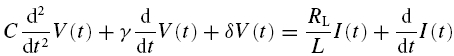with

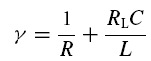and

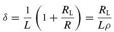For vanishing input current, I(t) = 0, the solution of this differential equation is given by:

where V₁ and V₂ are determined by the initial values of V and dV/dt and λ₁ and λ₂ are given by:

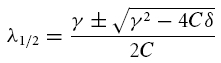The constant solution V(t) = 0 is stable, i.e. perturbations of V do not grow in time, if and only if the real parts of λ₁ and λ₂ are negative or zero. Inspection of eqn (A5) shows that two main dynamical regimes have to be distinguished (see also Fig. 8):

(A) If γ² − 4Cδ < 0, the square root in eqn (A5) has an imaginary solution which implies that any time-varying solution V(t) must exhibit oscillatory behaviour (see also Puil et al. 1986). Stability requires that these oscillations do not grow in time which is true if and only if γ ≥ 0. Under this condition, the solution eqn (A5) may be rewritten as

V₀ and ϕ₀ are constants to satisfy initial conditions, the decay factor λ is the real part of λ₁ in eqn (A5):

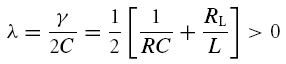and the oscillation or ‘natural’ frequency, f_nat, is given by imaginary part of λ₁:

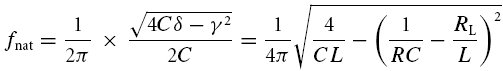(B) If γ² − 4Cδ ≥ 0, the square root has a real-valued solution, and as C > 0, the larger of the two λ values is negative or zero if and only if . Because the square root in eqn (A5) is non-negative in this scenario, γ has to obey γ ≥ 0. Solving and taking the positivity of C into account, we obtain a second necessary and sufficient condition, δ ≥ 0, which is not required in the first scenario (A). For completeness of this characterization, we denote by C the region of parameters that correspond to unstable solutions.

This analysis shows that a negative γ causes instability. On the other hand, stability does not imply positive L, R and R_L. However, for all cells analysed, the circuit parameters were positive. We therefore only treat this case in the following sections.

Resonance behaviour

Let us now derive the impedance–frequency curve needed to fit voltage traces obtained from measurements with ZAP input currents. To calculate the model response to a sinusoidal input with oscillation frequency f, we insert I(t) = I₀ exp(2iπft) into eqn (A1) and search for oscillatory solutions of the type V_theory(t) = V_theory(f) exp(2iπft). In terms of its amplitude A_theory and relative phase ϕ_theory, the complex-valued function V_theory(f) is given by V_theory(f) = A_theory(f) exp[iϕ_theory(f)]. Solving eqn (A1) leads to the theoretical impedance–frequency curve, defined as Z_theory(f) = V_theory(f)/I₀ (see also Hutcheon et al. 1996b):

The impedance Z_theory(f) decays with increasing frequency f if the circuit parameters obey:

If eqn (A10) is not fulfilled, the impedance has a maximum at a non-zero resonance frequency f_res:

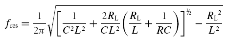Response to step-current inputs

To analyse the response to an external step-current input, let us assume that at t = 0, the current is stepped from 0 to the value I_step, i.e. I(t) = 0 for t < 0 and I(t) = I_step for t > 0. As we assume that the cell operates in its stable regime, the membrane potential will relax to a new value V_∞ for long times, so that dI/dt, dV/dt and d²V/dt² vanish in this limit. Equation (A1) then implies:

in accordance with the interpretation of ρ as the cell's input resistance.

Depending on the circuit parameters, the model shows qualitatively different transients before steady state is reached. In scenario (A), defined by γ² − 4Cδ < 0, solving eqn (A1) leads to

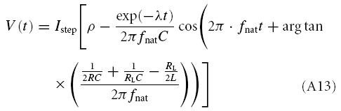where, as before, the membrane potential is measured relative to the holding potential. λ and f_nat are defined in eqns (A8) and (A9), respectively, and depend on the membrane potential. For small I_step one may, nevertheless, try to use values λ and f_nat obtained at the holding potential.

In scenario (B), defined by γ² − 4Cδ > 0, solving eqn (A7) leads to

where λ₁ and λ₂ are given by eqn (A5). As this solution involves the difference of two exponential functions, it can either have a single extremum (B-I) or decay without an extremum (B-II) (see also Richardson et al. 2003). The first case implies an overshooting membrane potential, so that V(t) = I_stepρ is obtained not only for t → ∞ but also at some finite t (see Fig. 8, insets 1–7). This occurs if the parameters allow the expression in square brackets in eqn (A13) to vanish for finite t which is true if and only if L > CRR_L. (There is a second condition, namely LC⁻¹ R_L⁻² > 0, but as the cell parameters were always positive, this constraint is not important here.)

With respect to step-current inputs, there are thus three qualitatively different classes of membrane-potential responses that relax to stable solutions (see also Fig. 8):

1.  multiple overshoots of the membrane potential whose amplitude decay in time.

2.  a single overshoot of the membrane potential, followed by a monotone decay.

3.  a monotone decay of the membrane potential without any overshoot.

Depending on the size of the decay factor λ and the cell's or measurement's noise level, the damped oscillations following the initial overshoot in scenario (A) may not be visible in a physiological recording. There is thus no clear-cut experimental distinction between response class (A) and (B-I) possible. As both scenarios show an overshooting membrane potential, they should be classified as sag potentials. Furthermore, as can be seen from Fig. 8, the existence of a sag potential (parameter regions A and B-I) implies an impedance resonance, but as the dashed line separating resonant from non-resonant behaviour lies above the B-I–B-II boundary, an impedance resonance does not imply the existence of a sag potential.

Note that the decay factor and natural frequency capture the neurone's response to brief or step-like perturbations, as used in the experiments. On the other hand, when the cell is exhibiting MPOs in response to ongoing fluctuations of ionic channel currents, the oscillation frequency f_osc is determined both by the intrinsic noise spectrum and the cell's resonance properties, as discussed in Results. Thus f_nat and f_osc differ in general.

Finally, an elaborate in-depth analysis of eqns (A8) and (A11) reveals that within region (A), the natural oscillation frequency f_nat is smaller than the resonance frequency f_res (Müller, 2000). In addition, the model exhibits a so-called Hopf bifurcation when λ vanishes; this occurs in the limit where R → ∞ and R_L → 0, corresponding to an undamped oscillator. Consequently, the stationary rest state loses its stability for λ = 0 and a periodic oscillation appears. At this very point f_res and f_nat become equal and obey:

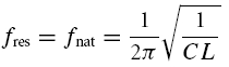Graphical representation of the different dynamical regimes

The time course of solutions generated by eqns (5) and (6) depends on L, C, R and R_L. For positive parameter values – true for all measured cells – the qualitative behaviour depends only on two combinations of the original parameters (Richardson et al. 2003), namely:

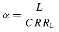and

This simplification allows us to visualize the different dynamical regimes in a two-dimensional representation, see, e.g. Fig. 8, and we obtain the following characterizations:

(A):

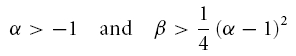(B-I):

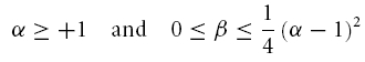(B-II):

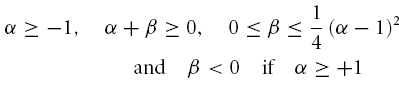In terms of α and β, condition (A10)reads:

In Fig. 8, the boundary (eqn (A21)) between resonant and non-resonant behaviour is shown as a dashed line. Note that this line differs from those separating the different dynamical regimes for responses to step-current inputs.

References

- Alonso A, Klink R. Differential electroresponsiveness of stellate and pyramidal-like cells of medial entorhinal cortex layer II. J Neurophysio. 1993;70:128–143. doi: 10.1152/jn.1993.70.1.128. [DOI] [PubMed] [Google Scholar]
- Alonso A, Llinas RR. Subthreshold Na+-dependent theta-like rhythmicity in stellate cells of entorhinal cortex layer II. Nature. 1989;342:175–177. doi: 10.1038/342175a0. [DOI] [PubMed] [Google Scholar]
- Amitai Y. Membrane potential oscillations underlying firing patterns in neocortical neurons. Neuroscience. 1994;63:151–161. doi: 10.1016/0306-4522(94)90013-2. [DOI] [PubMed] [Google Scholar]
- Bannerman DM, Yee BK, Lemaire M, Wilbrecht L, Jarrard L, Iversen SD, et al. The role of the entorhinal cortex in two forms of spatial learning and memory. Exp Brain Res. 2001;141:281–303. doi: 10.1007/s002210100868. [DOI] [PubMed] [Google Scholar]
- Bilkey DK, Heinemann U. Intrinsic theta-frequency membrane potential oscillations in layer III/V perirhinal cortex neurons of the rat. Hippocampus. 1999;9:510–518. doi: 10.1002/(SICI)1098-1063(1999)9:5<510::AID-HIPO4>3.0.CO;2-9. [DOI] [PubMed] [Google Scholar]
- Boulton CL, von Haebler D, Heinemann U. Tracing of axonal connections by rhodamine-dextran-amine in the rat hippocampal-entorhinal cortex slice preparation. Hippocampus. 1992;2:99–106. doi: 10.1002/hipo.450020203. [DOI] [PubMed] [Google Scholar]
- Bruehl C, Wadmann WJ. Calcium currents in acutely isolated stellate and pyramidal neurons rat entorhinal cortex. Brain Res. 1999;23:554–562. doi: 10.1016/s0006-8993(98)01234-7. [DOI] [PubMed] [Google Scholar]
- Buhl EH, Szilagyi T, Halasy K, Somogyi P. Physiological properties of anatomically identified basket and bistratified cells in the CA1 area of the rat hippocampus in vitro. Hippocampus. 1996;6:294–305. doi: 10.1002/(SICI)1098-1063(1996)6:3<294::AID-HIPO7>3.0.CO;2-N. [DOI] [PubMed] [Google Scholar]
- Buzsaki G. Theta oscillations in the hippocampus. Neuron. 2002;33:325–340. doi: 10.1016/s0896-6273(02)00586-x. [DOI] [PubMed] [Google Scholar]
- Chrobak JJ, Buzsaki G. Gamma oscillations in the entorhinal cortex of the freely behaving rat. J Neurosci. 1998;18:388–398. doi: 10.1523/JNEUROSCI.18-01-00388.1998. [DOI] [PMC free article] [PubMed] [Google Scholar]
- Cole KS. Membranes, Ions and Impulses. Los Angeles: University of California Press; 1968. [Google Scholar]
- Desmaisons D, Vincent JD, Lledo PM. Control of action potential timing by intrinsic subthreshold oscillations in olfactory bulb output neurons. J Neurosci. 1999;19:10727–10737. doi: 10.1523/JNEUROSCI.19-24-10727.1999. [DOI] [PMC free article] [PubMed] [Google Scholar]
- Dickson CT, Magistretti J, Shalinsky MH, Fransen E, Hasselmo ME, Alonso A. Properties and role of I(h) in the pacing of subthreshold oscillations in entorhinal cortex layer II neurons. J Neurophysiol. 2000a;83:2562–2579. doi: 10.1152/jn.2000.83.5.2562. [DOI] [PubMed] [Google Scholar]
- Dickson CT, Magistretti J, Shalinsky M, Hamam B, Alonso A. Oscillatory activity in entorhinal neurons and circuits. Mechanisms and function. Ann NY Acad Sci. 2000b;911:127–150. doi: 10.1111/j.1749-6632.2000.tb06723.x. [DOI] [PubMed] [Google Scholar]
- Dickson CT, Mena AR, Alonso A. Electroresponsiveness of medial entorhinal cortex layer III neurons in vitro. Neuroscience. 1997;81:937–950. doi: 10.1016/s0306-4522(97)00263-7. [DOI] [PubMed] [Google Scholar]
- Dugladze T, Heinemann U, Gloveli T. Entorhinal cortex projection cells to the hippocampal formation in vitro. Brain Res. 2001;905:224–231. doi: 10.1016/s0006-8993(01)02419-2. [DOI] [PubMed] [Google Scholar]
- Eder C, Ficker E, Gundel J, Heinemann U. Outward currents in rat entorhinal cortex stellate cells studied with conventional and perforated patch recordings. Eur J Neurosci. 1991;3:1271–1280. doi: 10.1111/j.1460-9568.1991.tb00060.x. [DOI] [PubMed] [Google Scholar]
- Eder C, Heinemann U. Current density analysis of outward currents in acutely isolated rat entorhinal cortex cells. Neurosci Lett. 1994;174:58–60. doi: 10.1016/0304-3940(94)90118-x. [DOI] [PubMed] [Google Scholar]
- Eder C, Heinemann U. Potassium currents in acutely isolated neurons from superficial and deep layers of the juvenile rat entorhinal cortex. Pflugers Arch. 1996;432:637–643. doi: 10.1007/s004240050180. [DOI] [PubMed] [Google Scholar]
- Egorov AV, Gloveli T, Muller W. Muscarinic control of dendritic excitability and Ca2+ signaling in CA1 pyramidal neurons in rat hippocampal slice. J Neurophysiol. 1999;82:1909–1915. doi: 10.1152/jn.1999.82.4.1909. [DOI] [PubMed] [Google Scholar]
- Empson RM, Gloveli T, Schmitz D, Heinemann U. Electrophysiology and morphology of a new type of cell within layer II of the rat lateral entorhinal cortex in vitro. Neurosci Lett. 1995;193:149–152. doi: 10.1016/0304-3940(95)11684-o. [DOI] [PubMed] [Google Scholar]
- Falk G, Fatt P. Linear electrical properties of striated muscle fibres observed with intracellular electrode. Proc R Soc Lond B Biol Sci. 1964;160:69–123. doi: 10.1098/rspb.1964.0030. [DOI] [PubMed] [Google Scholar]
- Galani R, Obis S, Coutureau E, Jarrard L, Cassel JC. A comparison of the effects of fimbria-fornix, hippocampal, or entorhinal cortex lesions on spatial reference and working memory in rats: short versus long postsurgical recovery period. Neurobiol Learn Mem. 2002;77:1–16. doi: 10.1006/nlme.2000.3998. [DOI] [PubMed] [Google Scholar]
- Gimbarzevsky B, Miura RM, Puil E. Impedance profiles of peripheral and central neurons. Can J Physiol Pharmacol. 1984;62:460–462. doi: 10.1139/y84-074. [DOI] [PubMed] [Google Scholar]
- Gloveli T, Dugladze T, Schmitz D, Heinemann U. Properties of entorhinal cortex deep layer neurons projecting to the rat dentate gyrus. Eur J Neurosci. 2001;13:413–420. doi: 10.1046/j.0953-816x.2000.01405.x. [DOI] [PubMed] [Google Scholar]
- Gloveli T, Egorov AV, Schmitz D, Heinemann U, Muller W. Carbachol-induced changes in excitability and [Ca2+]i signalling in projection cells of medial entorhinal cortex layers II and III. Eur J Neurosci. 1999;11:3626–3636. doi: 10.1046/j.1460-9568.1999.00785.x. [DOI] [PubMed] [Google Scholar]
- Gloveli T, Schmitz D, Empson RM, Dugladze T, Heinemann U. Morphological and electrophysiological characterization of layer III cells of the medial entorhinal cortex of the rat. Neuroscience. 1997a;77:629–648. doi: 10.1016/s0306-4522(96)00494-0. [DOI] [PubMed] [Google Scholar]
- Gloveli T, Schmitz D, Empson RM, Heinemann U. Frequency-dependent information flow from the entorhinal cortex to the hippocampus. J Neurophysiol. 1997b;78:3444–3449. doi: 10.1152/jn.1997.78.6.3444. [DOI] [PubMed] [Google Scholar]
- Gottesmann C. Theta rhythm: the brain stem involvement. Neurosci Biobehav Rev. 1992a;16:25–30. doi: 10.1016/s0149-7634(05)80047-8. [DOI] [PubMed] [Google Scholar]
- Gottesmann C. Detection of seven sleep-waking stages in the rat. Neurosci Biobehav Rev. 1992b;16:31–38. doi: 10.1016/s0149-7634(05)80048-x. [DOI] [PubMed] [Google Scholar]
- Gutfreund Y, Yarom Y, Segev I. Subthreshold oscillations and resonant frequency in guinea-pig cortical neurons: physiology and modelling. J Physiol. 1995;483:621–640. doi: 10.1113/jphysiol.1995.sp020611. [DOI] [PMC free article] [PubMed] [Google Scholar]
- Haas JS, White JA. Frequency selectivity of layer II stellate cells in the medial entorhinal cortex. J Neurophysiol. 2002;88:2422–2429. doi: 10.1152/jn.00598.2002. [DOI] [PubMed] [Google Scholar]
- Heinemann U, Schmitz D, Eder C, Gloveli T. Properties of entorhinal cortex projection cells to the hippocampal formation. Ann NY Acad Sci. 2000;911:112–126. doi: 10.1111/j.1749-6632.2000.tb06722.x. [DOI] [PubMed] [Google Scholar]
- Hille B. Ionic Channels of Excitable Membranes. Sunderland, MA: Sinauer; 1992. [Google Scholar]
- Hodgkin AL, Huxley AF. A quantative description of ion currents and ist application to condition and excitation in nerve membranes. J Physiol. 1952;117:500–544. doi: 10.1113/jphysiol.1952.sp004764. [DOI] [PMC free article] [PubMed] [Google Scholar]
- Hu H, Vervaeke K, Storm JF. Two forms of electrical resonance at theta frequencies, generated by M current, H current and persistent Na+ current in rat hyppocampal pyramidal cells. J Physiol. 2002;545:783–805. doi: 10.1113/jphysiol.2002.029249. [DOI] [PMC free article] [PubMed] [Google Scholar]
- Hutcheon B, Miura RM, Puil E. Subthreshold membrane resonance in neocortical neurons. J Neurophysiol. 1996a;76:683–697. doi: 10.1152/jn.1996.76.2.683. [DOI] [PubMed] [Google Scholar]
- Hutcheon B, Miura RM, Puil E. Models of subthreshold membrane resonance in neocortical neurons. J Neurophysiol. 1996b;76:698–714. doi: 10.1152/jn.1996.76.2.698. [DOI] [PubMed] [Google Scholar]
- Hutcheon B, Yarom Y. Resonance, oscillation and the intrinsic frequency preferences of neurons. Trends Neurosci. 2000;23:216–222. doi: 10.1016/s0166-2236(00)01547-2. [DOI] [PubMed] [Google Scholar]
- Jansen H, Karnup S. A spectral analysis of the integration of artificial synaptic potentials in mammalian central neurons. Brain Res. 1994;666:9–20. doi: 10.1016/0006-8993(94)90277-1. [DOI] [PubMed] [Google Scholar]
- Jones RSG. Synaptic and intrinsic properties of neurons of origin of the perforant path in layer II of the rat entorhinal cortex in vitro. Hippocampus. 1994;4:335–353. doi: 10.1002/hipo.450040317. [DOI] [PubMed] [Google Scholar]
- Koch C. Cable theory in neurons with active, linearized membrans. Biol Cybern. 1984;50:15–33. doi: 10.1007/BF00317936. [DOI] [PubMed] [Google Scholar]
- Koch C. Biophysics of Computation. Oxford: Oxford University Press; 1999. [Google Scholar]
- Lampl I, Yarom Y. Subthreshold oscillations and resonant behavior: two manifestations of the same mechanism. Neuroscience. 1997;78:325–341. doi: 10.1016/s0306-4522(96)00588-x. [DOI] [PubMed] [Google Scholar]
- Leung LS, Yu HW. Theta-frequency resonance in hippocampal CA1 neurons in vitro demonstrated by sinusoidal current injection. J Neurophysiol. 1998;79:1592–1596. doi: 10.1152/jn.1998.79.3.1592. [DOI] [PubMed] [Google Scholar]
- Lyons R. Understanding Digital Signal Processing. Menlo Park, CA: Addison-Wesley; 1998. [Google Scholar]
- Magistretti J, Alonso A. Biophysical properties and slow voltage dependent inactivation of a sustained sodium current in entorhinal cortex layer-II principal neurons: a whole-cell and single channel study. J General Physiol. 1999;114:491–509. doi: 10.1085/jgp.114.4.491. [DOI] [PMC free article] [PubMed] [Google Scholar]
- Markram H, Lubke J, Frotscher M, Sakmann B. Regulation of synaptic efficacy by coincidence of postsynaptic APs and EPSPs. Science. 1997;275:213–215. doi: 10.1126/science.275.5297.213. [DOI] [PubMed] [Google Scholar]
- Mauro A, Conti F, Dodge F, Schor R. Subthreshold behavior and phenomenological impedance of he squid giant axon. J General Physiol. 1970;55:497–523. doi: 10.1085/jgp.55.4.497. [DOI] [PMC free article] [PubMed] [Google Scholar]
- Metherate R, Cox CL, Ashe JH. Cellular bases of neocortical activation: modulation of neural oscillations by the nucleus basalis and endogenous acetylcholine. J Neurosci. 1992;12:4701–4711. doi: 10.1523/JNEUROSCI.12-12-04701.1992. [DOI] [PMC free article] [PubMed] [Google Scholar]
- Müller R. 2000. Neuronal dynamics and information processing: oscillation, resonance, and associative memory. PhD Thesis, Humboldt University, Berlin. [Google Scholar]
- Nelson PG, Lux HD. Some electrical measurements of motoneuron parameters. Biophys J. 1970;10:55–73. doi: 10.1016/S0006-3495(70)86285-3. [DOI] [PMC free article] [PubMed] [Google Scholar]
- Pike FG, Goddard RS, Suckling JM, Ganter P, Kasthuri N, Paulsen O. Distinct frequency preferences of different types of rat hippocampal neurones in response to oscillatory input currents. J Physiol. 2000;529:205–213. doi: 10.1111/j.1469-7793.2000.00205.x. [DOI] [PMC free article] [PubMed] [Google Scholar]
- Puil E, Gimbarzevsky B, Miura RM. Quantification of membrane properties of trigeminal root ganglion neurons in guinea pigs. J Neurophysiol. 1986;55:995–1016. doi: 10.1152/jn.1986.55.5.995. [DOI] [PubMed] [Google Scholar]
- Puil E, Gimbarzevsky B, Miura RM. Voltage dependence of membrane properties of trigeminal root ganglion neurons. J Neurophysiol. 1987;58:66–86. doi: 10.1152/jn.1987.58.1.66. [DOI] [PubMed] [Google Scholar]
- Puil E, Meiri H, Yarom Y. Resonant behavior and frequency preferences of thalamic neurons. J Neurophysiol. 1994;71:575–582. doi: 10.1152/jn.1994.71.2.575. [DOI] [PubMed] [Google Scholar]
- Richardson MJ, Brunel N, Hakim V. From subthreshold to firing rate resonance. J Neurophysiol. 2003;89:2538–2554. doi: 10.1152/jn.00955.2002. [DOI] [PubMed] [Google Scholar]
- Richter H, Heinemann U, Eder C. Hyperpolarization–activated cation current in stellate and pyramidal neurons of rat entorhinal cortex. Neurosci Lett. 2000;281:33–36. doi: 10.1016/s0304-3940(00)00794-1. [DOI] [PubMed] [Google Scholar]
- Schmitz D, Gloveli T, Behr J, Dugladze T, Heinemann U. Subthreshold membrane potential oscillations in neurons of deep layers of the entorhinal cortex. Neuroscience. 1998;85:999–1004. doi: 10.1016/s0306-4522(98)00113-4. [DOI] [PubMed] [Google Scholar]
- Shalinsky MH, Magistretti J, Ma L, Alonso A. Muscarinic activation of a cation current and associated current noise in entorhinal cortex layer II neurons. J Neurophysiol. 2002;88:1197–1211. doi: 10.1152/jn.2002.88.3.1197. [DOI] [PubMed] [Google Scholar]
- Steinmetz PN, Manwani A, Koch C, London M, Segev I. Subthreshold voltage noise due to channel fluctuations in active neuronal membranes. J Comput Neurosci. 2000;9:133–148. doi: 10.1023/a:1008967807741. [DOI] [PubMed] [Google Scholar]
- Tennigkeit F, Ries CR, Schwarz DW, Puil E. Isoflurane attenuates resonant responses of auditory thalamic neurons. J Neurophysiol. 1997;78:591–596. doi: 10.1152/jn.1997.78.2.591. [DOI] [PubMed] [Google Scholar]
- Torrence C, Compo GP. A practical guide to wavelet analysis. Bull Amer Meteor Soc. 1998;79:61–78. [Google Scholar]
- Ulrich D. Dendritic resonance in rat neocortical pyramidal cells. J Neurophysiol. 2002;87:2753–2759. doi: 10.1152/jn.2002.87.6.2753. [DOI] [PubMed] [Google Scholar]
- Van der Linden S, Lopes da Silva FH. Comparison of the electrophysiology and morphology of layers III and II neurons of the rat medial entorhinal cortex in vitro. Eur J Neurosci. 1998;10:1479–1489. doi: 10.1046/j.1460-9568.1998.00162.x. [DOI] [PubMed] [Google Scholar]
- Volgushev M, Chistiakova M, Singer W. Modification of discharge patterns of neocortical neurons by induced oscillations of the membrane potential. Neuroscience. 1998;83:15–25. doi: 10.1016/s0306-4522(97)00380-1. [DOI] [PubMed] [Google Scholar]
- Wang XJ. Ionic basis for intrinsic oscillations. Neuroreport. 1993;5:221–224. doi: 10.1097/00001756-199312000-00008. [DOI] [PubMed] [Google Scholar]
- White JA, Alonso A, Kay AR. A heart-like Na+ current in the medial entorhinal cortex. Neuron. 1993;11:1037–1047. doi: 10.1016/0896-6273(93)90217-f. [DOI] [PubMed] [Google Scholar]
- White JA, Klink R, Alonso A, Kay AR. Noise from voltage-gated ion channles may influence neuronal dynamics in the entorhinal cortex. J Neurophysiol. 1998;80:262–269. doi: 10.1152/jn.1998.80.1.262. [DOI] [PubMed] [Google Scholar]
- White JA, Rubinstein JT, Kay AR. Channel noise in neurons. Trends Neurosci. 2000;23:131–137. doi: 10.1016/s0166-2236(99)01521-0. [DOI] [PubMed] [Google Scholar]