Generalized Genomic Distance–Based Regression Methodology for Multilocus Association Analysis

Abstract

Large-scale, multilocus genetic association studies require powerful and appropriate statistical-analysis tools that are designed to relate genotype and haplotype information to phenotypes of interest. Many analysis approaches consider relating allelic, haplotypic, or genotypic information to a trait through use of extensions of traditional analysis techniques, such as contingency-table analysis, regression methods, and analysis-of-variance techniques. In this work, we consider a complementary approach that involves the characterization and measurement of the similarity and dissimilarity of the allelic composition of a set of individuals’ diploid genomes at multiple loci in the regions of interest. We describe a regression method that can be used to relate variation in the measure of genomic dissimilarity (or “distance”) among a set of individuals to variation in their trait values. Weighting factors associated with functional or evolutionary conservation information of the loci can be used in the assessment of similarity. The proposed method is very flexible and is easily extended to complex multilocus-analysis settings involving covariates. In addition, the proposed method actually encompasses both single-locus and haplotype-phylogeny analysis methods, which are two of the most widely used approaches in genetic association analysis. We showcase the method with data described in the literature. Ultimately, our method is appropriate for high-dimensional genomic data and anticipates an era when cost-effective exhaustive DNA sequence data can be obtained for a large number of individuals, over and above genotype information focused on a few well-chosen loci.

Modern genetics researchers have access to an unprecedented array of technologies and resources that can be used to identify and characterize the inherited basis of disease susceptibility. For example, the availability of high-throughput sequencing and genotyping technologies, the information on the locations of ∼10 million SNPs in Ensembl and related databases, and the recent release of allele-frequency and linkage disequilibrium (LD) information on >2 million SNPs by the International HapMap Project investigators have provided researchers with resources that should motivate them to pursue genetic association studies of complex, multifactorial traits and diseases, such as blood-pressure level and cancer. Unfortunately, the history of association studies that have been pursued to identify genetic variations that contribute to complex, multifactorial traits and diseases has been plagued by inconsistent results,1 making it unclear how future large-scale association studies that are based on the use of these resources will fare. In general, the reasons for the lack of replication among association studies of complex traits and diseases are well recognized and reflect the simple fact that the influence and identification of each particular gene or environmental factor influencing these traits and diseases are often obscured or confounded by the effects of other factors. More-specific reasons for a lack of replication include differences in the choice of polymorphic sites to study, the genetic background of the population(s) sampled, the definition of the phenotype used, and the analysis methods used to assess associations.

Each of the issues plaguing association studies has been dealt with in the literature, to some degree, and new strategies are emerging that may strengthen confidence in association studies. For example, strategies for identifying appropriate polymorphisms to consider in association studies have been described by researchers involved in the International HapMap Project.2 These strategies are based on the frequency of various alleles within and across populations, as well as the LD patterns that have emerged from analyses of them.2 In addition, methodologies for both uncovering and accommodating population-genetic background differences and potential cryptic substructure within a specific population are being developed, in an effort to avoid false-positive and false-negative association-test results attributable to the overall genetic heterogeneity of populations.3^,4 More-sophisticated phenotyping strategies are also being developed, with an emphasis on assaying subclinical endophenotypes that may more clearly reflect pathophysiological perturbations associated with a disease and that are influenced by inherited variations.5 The use of these phenotyping technologies is likely to accelerate the discovery of functionally relevant connections between particular genetic variations and subclinical phenotypes of all sorts.

One of the thorniest problem areas for association studies involves relating genotype information to phenotype information in relevant statistical-analysis models. Although many analysis models and tools have been proposed in the literature, many of those tools either have been developed as extensions of traditional statistical-analysis models, such as regression models, and, as such, have inherited whatever limitations these traditional models might have (e.g., assumptions of normality), or are rooted in the exploitation of LD relationships between observed marker-locus data and unobserved trait-influencing loci. This focus on analysis methods that exploit LD is most likely the result of the current expense of genotyping individuals at a large number of loci and, therefore, the need to be economical in the choice of loci to study. We consider a complementary data-analysis strategy for genetic association studies that is based on the assessment and analysis of the similarities and differences in the allelic composition of individual genomes and the relationship of these similarities/differences to phenotypic similarities/differences. This strategy has been developed with five phenomena—related to the human genome and human physiology—in mind that, if ignored, could create problems for human association studies. We outline these five phenomena below.

First, humans are diploid and, as such, the biological effect of a gene or genes on phenotypic expression likely involves the activities and actions of both gene copies simultaneously (e.g., consider recessive-allele effects for which two copies of the allele are needed to induce a phenotype). In this light, analysis strategies that consider merely the differences in the, for example, frequency of haplotypes or alleles between individuals with and without a phenotype may be ignoring biological realities of the combined effects of the genes on the maternally and paternally derived chromosomes each individual possesses. The analysis of diplotypes, as opposed to haplotypes, however, is starting to receive attention among statistical geneticists interested in association studies.6

Second, it is unlikely that individual variations observed at different positions in a gene or within a group of genes function in isolation. Rather, it is more likely that the net effect of multiple variable sites in a gene or set of genes influences phenotypic expression.7^,8 Thus, there are likely subtle (if not overt) interaction effects of multiple variations within a single gene on phenotypic expression that can be observed only if one considers the influence of these variations simultaneously in an analysis.

Third, the inheritance and the evolutionary history of a set of gene variations may not be of direct relevance to the phenotypic effect of those variations. Consider, for example, the very contrived and somewhat improbable possibility that two chromosomes, each developing the same set of de novo mutations that cause a phenotype, arose in different locales at quite different times. In this situation, the assumption of a single haplotype surrounding the causal allele would be inappropriate, and methods that exploit LD patterns and common haplotypes may not work in this setting. Many analysis methods for association studies that are designed to exploit LD seek to identify and assign haplotypes and haplotype categories to individuals on the basis of the ancestry of those haplotypes (i.e., the origins of the chromosomes or haplotypes transmitted to an individual from his or her parents and the relationships of those haplotypes to a putative ancestral set of haplotypes derived from a common ancestor). However, the actual mutational or sequence profile or combination of variations in a gene and its regulatory elements are of greater relevance to association studies than are the ancestry of those variations, and the real problem lies in identifying and separating the functional variations from the neutral variations, with respect to a particular phenotype.

Fourth, each individual is likely to have his or her own unique genetic signature or combination of variations. Consider the fact that the more polymorphic sites a researcher considers in an association analysis, the greater the likelihood that each individual in the study will possess a unique pattern of variations at those sites. Thus, it is important to try to develop analysis methods for reducing the number of contrasts to be made in an association study by grouping individuals together on the basis of the common or shared variations they possess.

Fifth, studies investigating the in vitro and in silico functional significance of genes and genetic variations are being pursued on a large scale. These studies can shed light on polymorphic sites in the genome that are of direct relevance to a particular trait or disease.9^–11 In fact, a number of computational tools have been developed to help distinguish variations of likely functional significance on the basis of, for example, amino acid changes in an encoded protein, position in a splice site of a gene, or position in a transcription-factor binding site (TFBS).12^–15

The association-analysis methodology that we describe attempts to address these issues by taking a more holistic multilocus diplotype view of the phenotypic effects of variations within a gene7^,16^–18 and does not consider the analysis of variations as single independent factors within a gene. Our proposed association methodology considers the relationship between variation in the similarity of the allelic profile (based on alleles at polymorphic loci) among a group of individuals and additional information collected about those individuals. In this light, our methodology addresses questions such as: How much of the genomic similarity assessed with respect to variations in a particular genomic region exhibited by a group of individuals can be explained by their disease statuses and relevant ancillary information? Or, rather, is it the case that individuals with a disease or elevated values of a particular phenotype have similar genomes or genomic profiles in a region of interest that is unlikely to have arisen by chance? The method critically depends on measures of genomic similarity and dissimilarity, or “distance.” These measures can be constructed in such a way as to accommodate and/or address the five aforementioned genomic and physiologic phenomena not often explicitly addressed in traditional association-study data-analysis methodologies.

In describing the method, we consider the derivation of different measures of genomic dissimilarity, or distance, taking into account different features of genetic variations for each measure. We then consider the derivation of a test statistic that relates genomic dissimilarity to phenotypic end points (e.g., diagnosis, quantitative level of a phenotype, etc.). Unlike other methods, our method does not require clustering individuals into groups—which can be problematic for a number of reasons, not the least of which concerns the number of groups one should consider as present in the data. In this light, our approach is similar in orientation to the approach outlined in the derivation of the analysis of molecular variance (AMOVA) strategy of Excoffier et al.19 However, unlike the AMOVA approach, the formulation of the model and test statistics we use are more flexible and can be used to assess multiple phenotypes, covariates, and a priori population groupings, as briefly outlined in the “Subjects and Methods” section. Our proposed method encompasses and can be used to generalize single-locus and haplotype-phylogeny analysis methods, in that one can pursue both single-locus analyses and haplotype-phylogeny analyses with the proposed procedure, as described in the “Subjects and Methods” section. In this light, our method is at least as powerful as those methods but provides possible extensions that can accommodate settings and locus effects that traditional approaches cannot. Thus, our proposed method can only improve traditional single-locus analysis of variance (ANOVA) and haplotype-phylogeny analysis methods. We describe data sets used to showcase the proposed techniques and the results of relevant analyses of these data sets. We end with a discussion and considerations of areas for future research.

Subjects and Methods

Measures of Genomic Similarity

There are a number of strategies for characterizing the similarity of individuals with respect to the variations they possess, both within and across different genes. We describe seven example methods for assessing the genomic similarity between two individuals on the basis of genotype data. Some of these methods have been designed to accommodate weighting schemes for various factors, such as allele frequency or locus functional significance. In addition, it is possible that combinations of the approaches could be pursued (e.g., weighting by both frequency and function). Weighted similarity measures have been extensively studied in cluster-analysis contexts and so are appropriate to consider in other contexts.20 Once a similarity measure has been chosen, it can be evaluated for all pairs of N individuals in a sample, to construct an N×N similarity matrix, where element i,j of that matrix contains the similarity value for individuals i and j (i,j=1,…,N). We note that other groups have considered different measures of genomic similarity that may be of value21 (see, e.g., the works by Müller et al.22 and by Sielinski23). We also note that similarity matrices admit intuitive graphical representations in the form of heat maps and trees,24^–26 which makes our proposed analysis procedure intuitively appealing, as described below (see also figs. 1 and 2).

Figure 1. .

Heat-map representations of the similarity in the allelic profiles of 57 unrelated CEPH individuals based on variations in the CHI3L2 gene (A) or the SQSTM1 gene (B), with use of a standard IBS allele-sharing measure. Note that individuals have been ordered in the matrix by increasing CHI3L2 levels. The concentration of red cells in the matrix along the diagonal in panel A suggests an association between similarity in CHI3L2 gene composition and CHI3L2 expression. The lack of a pattern in panel B suggests that no association exists between similarity in SQSTM1 gene composition and CHI3L2 expression.

Figure 2. .

Tree representation of the similarity in the allelic profiles of 57 unrelated CEPH individuals based on variations in the CHI3L2 gene with use of a standard IBS allele-sharing measure. The proximity of the branches associated with individuals corresponds to greater similarity. Individual branches are coded such that, the larger the number, the greater the CHI3L2-expression value an individual has. It can be seen that individuals with similar number codes (i.e., individuals with similar CHI3L2-expression values) are on branches near each other (in general), which is indicative of the association between greater CHI3L2 allelic–composition similarity and CHI3L2 gene–expression level.

Similarity based on identity-by-state (IBS) allele sharing

The fraction of alleles that any two individuals share purely by state (e.g., the two individuals possess the same allele or variant at a locus) can be calculated easily enough. Since humans have two copies of each position on the genome, it is simple to determine how many alleles (0, 1, or 2) a pair of individuals shares. By dividing by twice the number of loci or positions studied, one can obtain an estimate of the fraction of alleles shared IBS by those individuals. Pairwise similarities derived in this manner have been used to construct a matrix for cluster (and related) analyses, to address population genetic research questions.27^,28 The IBS-sharing similarity, S_i,j, can be calculated for individuals i and j (i,j,=1,…,N) with the formula

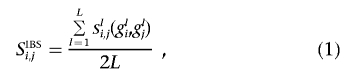where L is the number of loci considered in the calculation; g^l_i and g^l_j are the genotypes of individuals i and j, respectively, at the lth locus (l=1,…,L); and s^l_i,j(g^l_i,g^l_j) is a function mapping the genotype information, for individuals i and j at locus l, to a particular numeric value and, for our purposes, has a value of 0.0 if individuals i and j are homozygous for different SNP alleles (e.g., g^l_i=AA and g^l_j=TT), a value of 1.0 if they share one allele (e.g., g^l_i=AA and g^l_j=AT), and a value of 2.0 if they share both alleles (e.g., g^l_i=AA and g^l_j=AA)—note that we are assuming, throughout, that interest is in SNP loci with two alleles, as opposed to microsatellite markers and other forms of genetic variation, although the proposed method can be easily extended to cover situations in which those forms of variation are examined.

Similarity based on weighting by allele frequency

Allele-frequency information can be included in the construction of the measure of similarity. The intuition behind the accommodation of allele frequency is that individuals who share rare alleles may have more-similar genomes than do individuals who share common alleles (i.e., since many people will have common alleles, individuals possessing them are not easily distinguished from others). Lynch and Ritland devised a method (hereafter called “the LR method”) for assessing genomic similarity, on the basis of genotype data, that accounts for allele frequency and has been shown to have some favorable properties for identifying population subgroups.21^,29^,30 With notation derived from equation (1), weighted similarity measures can be computed easily as

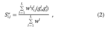where w^l is a positive number reflecting the weight assigned to locus l.

IBS allele sharing, with weighting for functionality of variations

One can accommodate knowledge of the “functional significance” of variations in a measure of genomic similarity by giving greater weight in the sharing measure to loci harboring functional variations. These weights must be determined a priori and can be based on, for example, the results of cellular in vitro assays investigating the influence of variations on gene expression or protein-binding potential. As an example, consider a situation in which in vitro functional-analysis assays suggest that variations at two polymorphic sites in the promoter region of a gene resulted in a 1.5-fold and a 2.0-fold increase in expression levels and that a variation at another polymorphic site resulted in a protein amino acid change that causes a binding site in that protein to induce a 2.0-fold increase in activity of the protein. In this hypothetical situation, one could assign weights of 1.5, 2.0, and 2.0, respectively, to the loci harboring these variations, in the construction of the similarity measure.

Similarity based on weighting by nucleotide conservation across species

In the absence of data on the potential functional effect of variations, one could consider a criterion for weighting loci in a genomic similarity measure that is based on conservation of nucleotides across species. It has been argued that nucleotides that are conserved throughout evolution are more likely to be of functional significance, since changes at those positions may have undergone negative selection; see, for example, the works of Shah et al.,31 Frazer et al.,32 and Brudno et al.33 Thus, one could weight genomic positions used in a genotype-based similarity measure by the degree of evolutionary conservation at those positions.

Similarity based on single-locus–analysis results

We consider the use of single-locus–analysis results in the construction of a multilocus similarity measure. Single-locus analyses can be pursued before the construction of a similarity measure or could be based on analyses performed previously with another data set. We consider the use of the negative log of the P value associated with single-locus–analysis test statistics as weights in the construction of a similarity measure using, for example, equation (2) or equation (3).

Unweighted and weighted haplotype-pair similarity

By phasing individuals (i.e., assigning them haplotypes that reflect variations they inherited on their maternally and paternally derived chromosomes), one can assess the similarity of two individuals’ chromosome pairs. A relevant similarity measure would depend critically on how one pairs (or matches) the chromosomes between the two individuals, since the similarity could be very different for the two possible pairings. A better measure would involve computing the similarity with the assumption of both pairings and then taking the maximum measure that results from these two pairings as the measure of similarity. Consider, for example, the simple situation in which individual a has haplotypes ha1=0-0-0-0 and ha2=1-1-1-1 and individual b has haplotypes hb1=1-1-1-1 and hb2=0-0-0-0. Then, to assess haplotype similarity, if one pairs ha1 with hb1 and pairs ha2 with hb2, the individuals would have completely different genomes (i.e., have maximal distance, or zero similarity). However, if one pairs ha1 with hb2 and pairs ha2 with hb1, then the individuals have identical genomes. We believe that use of the pairing that maximizes the similarity is appropriate, and that was the motivation for the measure reflected in equation (3). Haplotype-based sharing can easily accommodate weighting schemes based on, for example, conservation or functionality, in which some loci have been weighted because of their putative functionality. Although slightly more complicated than the genotype similarity–based measures, haplotype pair–similarity measures can be computed as

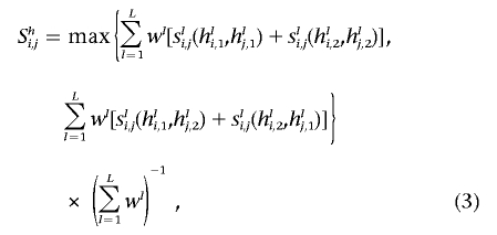where the similarity function considers the alleles on specific haplotypes possessed by individuals i and j and would assign a numerical value of 0.0 if the individuals did not have the same allele on those haplotypes and 1.0 if they did (note that, in eq. [3], h^l_i,1 refers to individual i’s allele at position l of his or her chromosome designated as 1, as opposed to 2). In addition, the fact that one could pair the first haplotype (arbitrarily defined) possessed by individual i with either the first or the second haplotype possessed by individual j is accommodated in the calculation by use of the maximum of these two pairings to define the similarity.

Similarity based on ancestry

There are many association-analysis methods that consider similarity in the phylogenetic connections or ancestry of haplotypes.34^–37 For example, the programs eHAP,35^,38 HAP,39 Arlequin,40 and GeneTree,41 produce phylogenies of chromosomes on the basis of genotype data. The phylogenies produced by these programs can then be used to group individuals into smaller subgroups that can be used to contrast phenotypic features. We consider this approach as an alternative to those that are based on, for example, functional-variation similarity, although recent studies have suggested that grouping haplotypes on the basis of phylogeny and then contrasting the resulting groupings for phenotypic differences does not substantially increase power to detect an effect (see, e.g., the work of Humphreys and Iles42 and Bardel et al.43). However, we note that one can exploit ancestral relationships between haplotypes to derive a similarity measure. Essentially, from a phylogenetic tree, one can determine the distance between haplotypes (e.g., on the basis of the number of mutations, recombinations, gene conversions, or transitions that must have occurred to derive one haplotype from another ancestral haplotype) (see fig. 3). With this information, one can pair the haplotypes that two individuals possess and can compute the phylogenetic distance between those haplotypes. Since this pairing can occur in two ways, we take the pairing that produces the minimum distance between the two individuals as reflecting the similarity between them, as was done for the haplotyping pairing–similarity measures discussed above.

Figure 3. .

A, Tree representation of the phylogenetic relationships of haplotypes derived from the CHI3L2 genotype data for the 57 unrelated CEPH individuals, with use of the method of Seltman et al.35^,38 B, The distance matrix used to construct the phylogenetic tree, with the numbers on the rows and columns identifying the different haplotypes. Note that the haplotypes are identified with numbers assigned arbitrarily (C). Haplotypes that are phenotypically similar are denoted by their corresponding symbols.

Regression-Based Distance Matrix Analysis

Once one has computed a similarity matrix, that matrix can be subjected to a regression analysis that tests hypotheses about whether variation in the level of similarity exhibited by pairs of individuals reflected in that matrix can be explained by other features those individuals possess (e.g., whether they possess a certain phenotype or have higher or lower values of a particular quantitative phenotype). To describe the regression model, we consider an analysis involving a gene or genomic region that harbors L different polymorphic loci. We also assume that each of N individuals or study subjects has been genotyped at these L loci. We assume also that M phenotypic variables have been collected on the N subjects. These phenotypic variables could include information about the presence or absence of a disease end point (e.g., coded using dummy variables, such as 0 assigned to individuals without the disease and 1 assigned to individuals with the disease); disease-associated quantitative variables, such as blood pressure and cholesterol level; and important covariates, such as age, sex. smoking status, etc. We assume that interest is in relating the disease end points or quantitative variables to the genomic profiles of the individuals, as captured by the genotypic information collected about them.

Construct an N×N similarity matrix with, for example, one of the measures described in the “Measures of Genomic Similarity” section. Transform the matrix into a dissimilarity, or “distance,” matrix by, for example, subtracting the components of the matrix from 1.0 if the IBS measure is used or by subtracting them from 1.0 after each component in the matrix is divided by the theoretical or empirical maximum of the similarity measure, to scale the entries to lie between 0 and 1. We note that the proposed regression procedure does not require that the distance matrix have metric properties.44 Let this distance matrix and its elements be denoted by D=d_ij (i,j=1,…,N), for the N subjects. The possibility that N≪L will not pose problems in the proposed regression-analysis setting. Let X be an N×M matrix harboring information on the M phenotypic variables that will be modeled as predictor or regressor variables whose relationships to the values in the genomic similarity matrix are of interest. Compute the standard projection matrix, H=X(X^′X)^-1X^′, typically used to estimate coefficients relating the predictor variables to outcome variables in multiple-regression contexts. Next, compute the matrix

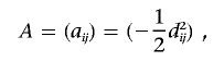center this matrix with use of the transformation discussed by Gower,45 and denote this “matrix G” as

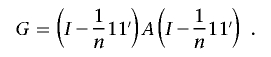An F statistic can be constructed to test the hypothesis that the M regressor variables have neither relationship to variation in the genomic distance nor dissimilarity of the N subjects reflected in the N×N distance/dissimilarity matrix as done by McArdle and Anderson46:

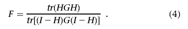If the Euclidean distance is used to construct the distance matrix on a single quantitative variable (i.e., as in a univariate analysis of that variable) and appropriate numerator and denominator degrees of freedom are accommodated in the test statistics, then the F statistic in equation (4) is equivalent to the standard ANOVA F statistic.46 The distributional properties of the F statistic are complicated for alternative distance measures computed for more than one variable, especially if those variables are discrete, as in genotype data. However, permutation tests can then be used to assess statistical significance of the pseudo–F statistic.44^,46^–50 The M regressor variables can be tested individually or in a stepwise manner.

Graphic Display of Similarity Matrices

Similarity matrices of the type we describe can be represented graphically in a number of ways that can facilitate interpretation. We consider heat-map and coded-tree (or dendogram) representations.24^–26 Heat maps simply color code the elements of a similarity matrix, such that higher similarity values are represented as “hotter,” or redder colors, and lower similarity values are represented as “colder,” or bluer colors. If the matrix is ordered such that individuals with similar phenotype values are next to each other, then neighboring cells along the diagonal of the matrix (representing individuals with similar phenotype values) will present patches of red, indicating a relationship between the phenotype values and similarity (fig. 1A and 1B). Trees are constructed such that individuals with greater genomic similarity are placed next to each other (i.e., they are represented as adjacent branches of the tree). Less similar individuals are represented as branches some distance away from each other. By color coding the individual branches on the basis of the phenotype values of the individuals they represent, one can see if there are patches of a certain color on neighboring branches, which would indicate that phenotype values cluster along with genetic similarity (fig. 2)

The CEPH Family Gene-Expression Data as an Example Data Set

To showcase the proposed method relative to other methods, we considered an analysis involving gene-expression and SNP data collected on 57 unrelated CEPH individuals. These individuals were chosen by HapMap researchers for massive, genomewide genotyping studies2 and were also used to assess gene-expression patterns obtained from immortalized lymphocytes51 (Gene Expression Omnibus accession number GSE2552). Our analysis excluded individual NA06993 in the gene-expression studies, because detailed analysis of HapMap data suggested that the sample associated with this person is likely to have derived from an unreported relative. We also added data associated with individual NA12056, since gene-expression data for this individual is now available. We focused on the analysis of variations genotyped on the CEPH individuals in the CHI3L2 gene (MIM 601526), since Cheung et al.51 found very compelling evidence of association and linkage to this gene for the expression levels of the CHI3L2 gene, reflecting likely cis-acting sequence variations influencing expression of the encoded protein. We downloaded, from the HapMap database, data on 43 SNPs in the CHI3L2 gene that were genotyped on the 57 CEPH individuals with CHI3L2 gene–expression values (chromosome 1: 111069007–111084786; Ensembl position 111482322–111498101). We derived the positions of the SNPs from the latest version of the human physical map provided in Ensembl. We note that these positions disagree slightly with those reported by Cheung et al.51

Haplotyping and Basic Analysis of the Expression Data

Haplotypes and diplotypes (i.e., the pairs of haplotypes each individual possesses) were inferred using HAP.39 Repeated, multiple gene–expression values collected for each of the CEPH individuals were averaged, when available. We considered use of log₂-transformed expression levels because of skewness in the expression values. We assessed the association between the SNPs in the CHI3L2 gene and CHI3L2 gene–expression values, using regression analysis of each, coded as 0, 1, or 2, depending on how many minor alleles each individual possessed at a SNP locus. We also tested for haplotype associations, using the haplotype-phylogeny–analysis methods described by Seltman et al.35^,38 We then applied the proposed analysis method using different similarity measures. We also included analyses that considered each locus in isolation, using the proposed similarity-regression procedure—that is, we constructed the similarity matrix using genotype information for each locus independently. To correct for multiple testing in the single-locus analyses, we used the method developed by Nyholt,52 to determine the “effective” number of independent SNPs from the total of 26 that we studied. The effective number of independent SNPs was found to be ∼14. We then used a Sidak-corrected P value to declare significance at the nominal level of P<.05. For the distance-based regression analysis, we used 100,000 permutations of the data to assess the probability of a type I error. We considered sex as a covariate in the analysis methods used.

Assessing SNP Functional Significance for Similarity-Measure Weighting

For the proposed similarity measure exploiting functional information on the SNPs, we considered the use of a number of resources, including results of in vitro studies, (e.g., promoter-reporter cell transfection and/or model species analyses), in silico (computational) structure and sequence analysis, and sequence-conservation analyses. We considered SNPs in all the genetic regions that were available—for example, putative functionally relevant SNPs, such as coding (synonymous and nonsynonymous) and noncoding (exonic splicing enhancers [ESEs] and TFBSs, in both the 5′ and 3′ UTRs), as well as likely neutral variations, such as SNPs in functionally obscure intronic sites. We used available Web-based tools and programs to assess functionality (see table 1, which describes the analysis tools and references for our assessment of functionality and conservation). To complement the information we obtained from individual Web sites, we used PupasView, a Web site that gives comprehensive functional information from many individual programs and databases. To assess evidence of evolutionary sequence conservation at the site harboring each SNP, we leveraged data from multiple species. Genomic regions that show evidence of multiple-species sequence conservation at the nucleotide level are more likely to have undergone selective pressures and, hence, are likely to be of functional significance.53 Use of multiple-species genomes in comparisons with the human sequence (as the reference genome) has the advantage of providing stricter criteria, which minimizes false-positive conservation results with any one species and improves the ability to classify elements as actively conserved because of functional consequences rather than shared ancestry. For weighting based on sequence conservation, sites had to be identified as conserved in two or more species to be given a greater weight; when sites were found conserved across more than two species, more weight was given. In using functional information to weight the SNPs in a similarity measure, we intentionally kept our weighting scheme simple so as not emphasize the absolute value of the weight; rather, the weighting was relative to each SNP. We felt that the most weight should be given to SNPs characterized as functional by in vitro methods (e.g., SNP rs755467=2.0) (see table 2). If multiple in silico methods identified a SNP as having plausible functional consequence, then more weight was given to that SNP than to those for which only one method suggested functionality. In addition, because of imprecision in the computational identification of regulatory binding motifs, we required agreement among programs used for identifying a sequence as being in a TFBS, a UTR, or an ESE, to reduce false-positive results.

Table 1. .

Resources for Identifying or Predicting Function and Conservation in CHI3L2

Reference	Function	Comment
Cheung et al.51	In vitro	Twofold increased binding of RNA polymerase II (T→G allele)
PupasView	Comprehensive
SIFT	Nonsynonomous SNPs	Sorting Intolerant from Tolerant
PolyPhen	Nonsynonomous SNPs
ESEfinder	ESEs
RESCUE-ESE	ESEs
Gene Regulation	TFBSs	For P-Match
Vista Tools	TFBSs	For rVISTA
UTRScan	UTR functional elements
ITB Blast	UTR functional elements	For BigBlast
VISTA Genome Browser	Conservation
PipMaker and MultiPipMaker	Conservation	For PipMaker

Table 2. .

Characteristics of CHI3L2 SNPs, Functional Consequences, and Conservation^[Note]

SNP	Ensembl Position	Location	Minor-Allele Frequency	HWE P	tSNP	ESEfindera	RESCUE-ESEa	Functional Weight	Frog	Chicken	Mouse	Cow	Opossum	Dog	Fugu	Chimpanzeeb	Conservation Weight
rs755467c	111482465	Intron 1	.28	.739	N		Y (1)	2				62				99	1.15
rs2147790	111482633	Intron 1	.16	.082	N			1				62				99	1.15
rs2255089	111485610	Intron 3	.46	.253	N	Y (1)		1	34			63	20		18	97	1.30
rs2274232	111485642	Intron 3	.11	.003	N		Y (1)	1	34		63	63	20		18	97	1.45
rs2147789	111485872	Intron 3	.44	.025	Y		Y (3)	1	34			63	29			100	1.25
rs2182115	111486179	Intron 4	.09	.011	N	Y (2)		1	26		33	64	28			98	1.30
rs1325284	111487834	Intron 4	.33	1.000	N	Y (1)	Y (3)	1.5				70	28			98	1.65
rs2251715	111490229	Intron 5	.44	.274	N			1				72	35			98	1.50
rs961364d	111490510	Intron 6	.26	.613	N	Y (1)	Y (1)	1.75	19		19	71	42	31		99	1.70
rs2764543	111491140	Intron 7	.31	.771	N			1				68				98	1.15
rs7366568	111491806	Intron 7	.25	.020	N	Y (4)		1			24					98	1.10
rs2820087	111492376	Intron 7	.28	.975	N		Y (2)	1	37							98	1.10
rs6685226	111492646	Intron 7	.17	.142	N	Y (1)		1	51	70						98	1.35
rs11583210	111493928	Intron 8	.25	.075	Y			1	29		30	73	28	25		98	1.60
rs12032329	111494414	Intron 8	.12	.003	N		Y (2)	1	29		30	71				98	1.55
rs2477578	111495313	Intron 8	.33	1.000	N	Y (1)		1	29			71			13	98	1.55
rs2494006	111495483	Intron 8	.28	.956	N	Y (2)		1	29			71				98	1.50
rs7542034e	111496023	Thr313Thr	.02	.888	N	Y (3)		1.35	60		62	88	79		61	97	1.75
rs942694	111496180	Intron 9	.33	1.000	N			1	30		16	52	25			98	1.30
rs942693	111496200	Intron 9	.33	1.000	N	Y (2)		1	30		16	52	25			98	1.30
rs2182114	111496269	Intron 9	.33	1.000	N	Y (1)		1	30		16	52				98	1.40
rs5003369	111496447	Intron 9	.33	1.000	Y	Y (1)		1	30			52				98	1.20
rs11102221	111496858	Intron 9	.26	.161	N		Y (1)	1	30			71	38			98	1.55
rs3934922	111497436	Intron 10	.30	.556	Y	Y (3)	Y (2)	1.25	34					72		99	1.50
rs3934923	111497509	Intron 10	.33	1.000	N	Y (1)		1	34					72		99	1.65
rs8535	111497971	Exon 10	.28	.739	N	Y (1)		1	32					64		100	1.20

Note.— In silico results from UTR, TFBS, and nonsynonomous SNPs are omitted, since no functional SNPs were identified. Twelve species were considered in VISTA Genome Browser, five with high conservation (>70% identity). Fifteen species were considered in PipMaker; Drosophila results from PipMaker were omitted (62% conservation at rs7542034).

^aThe number of sequence motifs identified by the ESEfinder and RESCUE-ESE programs is shown in parentheses.

^bChimpanzee results are combined from VISTA Genome Browser and PipMaker.

^cIn vitro results showed 2 times greater binding by RNA polymerase II to the T allele, compared with the G allele.

^dPupasView finding was a triplex, a possible regulatory element.

^ePupasView finding was an ESE (3).

Results

Polymorphic Variation in CHI3L2

In CHI3L2, 11 SNPs were monomorphic, and 6 SNPs were excluded because of low minor-allele frequency (<2.0%) (data not shown). Five SNPs were not in Hardy-Weinberg equilibrium (HWE) (P<.05) (table 2). Because of the thorough quality assessment and control of the data by the HapMap researchers, we assumed that those SNPs not exhibiting HWE were not an artifact of genotyping; therefore, we opted to keep them in the analyses but also conducted analyses that excluded those SNPs. Four SNPs were tagging SNPs (tSNPs), on the basis of HapMap analyses. Five SNPs in the CHI3L2 gene were coding SNPs, as reported to dbSNP, one of which was genotyped by the HapMap researchers. The other SNPs were in noncoding or regulatory regions. The majority of the SNPs were in strong LD (average D^′=0.97), with the exception of SNP Thr313Thr, which showed weaker LD (D^′=0.02–0.80) with nine other SNPs (data not shown but easily visualized on the HapMap site).

SNP Functionality and Sequence Conservation Assessment Results

In Vitro and In Silico Analysis of CHI3L2 Variation

Promoter activity of luciferase reporter assays containing the rs755467 SNP was twofold higher (T→G allele) than that of constructs not containing the rs755467 SNP. This increase in promoter activity was because of stronger binding of RNA polymerase II.51 Four SNPs were identified, through in silico methods, as being in potential ESE sites (table 2). Although analyses involving the Web site PupasView found results similar to the analysis results based on other Web-based tools, it also uniquely identified a triplex, a possible regulatory element. UTRScan and BIGBlast did not identify any SNPs in UTR-binding motifs, and, similarly, P-Match (Gene Regulation) and rVISTA (Vista Tools) did not identify any TFBSs (results not shown). There were no nonsynonomous SNPs for evaluation.

Sequence Conservation Analysis of CHI3L2 Variation

VISTA browser2 (VISTA Genome Browser) was used to compare the sequence of CHI3L2 (chromosome 1: 111482202–111498000) from human (reference genome, May 2004 build, except that the chimpanzee sequence was compared with the July 2003 build) with 10 other available species. Overall, the amount of highly conserved sequence decreased with increasing phylogenetic distance. Chimpanzee, cow, dog, opossum, and fugu exhibited some highly conserved regions with humans; chimpanzee had the largest number of conserved sequences, and fugu had the least (>70% identity) (note that fugu has conserved sequence but does not contain any of the SNPs investigated in the present study). When we reduced to 5% the allowable percentage of identity for analysis, there was moderate conservation with mouse, frog, and chicken, and there was no conservation with rat or zebra fish. PipMaker and MultiPipmaker were also used for pairwise and multiple-species comparisons and to extend to different species not available at the VISTA Genome Browser Web site. PipMaker and VISTA Genome Browser pairwise comparisons gave slightly different results because of the different algorithms used (local vs. global homology, respectively). Only VISTA Genome Browser results are shown. Nine SNPs were in highly conserved regions in two or more species, whereas some conservation was found with other species (table 2). For comparisons involving a species more evolutionarily distant from humans, we studied sequence from Drosophila melanogaster. We found that only one SNP, Thr313Thr—the SNP that was most consistently conserved across multiple species—was in a conserved region, which suggests it might be a functionally important region for this gene. Anopheles gambiae was compared with human, and no conserved sequences were identified (data not shown). Comparison across multiple species, which can identify conserved regions possibly under selection, revealed SNPs with sequences conserved across multiple species and with more-distant species (rs7542034 and rs2255089).

To assign weights that were based on this information, we used a minimum identity of 70% to locate SNPs that were in highly conserved regions. Then, we lowered the minimum threshold to 5%, to identify regions of moderate conservation (40%–69%) or low conservation (10%–39%). Under the assumption that the in vitro results give the most-compelling results, our conservation weighting was scaled from 1 to 1.75, where 1 is no conservation across multiple, pairwise species comparisons and 1.75 is the most conserved region (with high conservation and the most species) and represents a value less than those of the in vivo results. We categorized conservation levels as high, moderate, or low and used this scheme to assign weights to the loci. We recognize that our scheme for assigning weights may seem arbitrary, but we chose to expose the use of weights that are based on different criteria and not necessarily to focus on the optimal manner in which weights can be assigned.

Single Locus–Analysis Results

Of the 26 SNPs, 14 were significantly (i.e., P⩽.001) associated with CHI3L2 log₂-transformed expression levels after correction for multiple tests (note that none of these analyzed SNPs deviated from HWE) (table 3 [columns 3–6]). In addition, two of the four SNPs identified as tSNPs, according to the HapMap Web site, were significantly associated with CHI3L2 levels. We also include in table 3 the results of the single-locus analyses with use of the proposed similarity-analysis approach (columns 7–10), and, as can be seen, the single-locus results with the proposed procedure correspond well with results obtained from the traditional regression-based single-locus analysis. We note that the Spearman rank correlation between the P values obtained from these two analyses was 0.862 (P<.0001). Thus, our proposed procedure can be used to conduct single-locus analyses.

Table 3. .

Individual SNP Associations with CHI3L2 Expression Levels^[Note]

		Traditional Regression Analysis					Similarity Regression Analysis
SNP	Location	F	Exact P	Corrected Pa	Variation (%)	(−)log10 P	IBS F	IBS P	Variation (%)
rs755467	Intron 1	15.57	4.58×10-6	.00006	37	4.19	3.71	.00001	36
rs2147790	Intron 1	.28	7.53×10-1	1.00000	1	.00	.17	.68502	00
rs2255089	Intron 3	3.68	3.16×10-2	.36208	12	.44	6.49	.01408	11
rs2274232	Intron 3	1.01	3.70×10-1	.99845	4	.00	2.01	.16097	4
rs2147789	Intron 3	5.44	7.70×10-3	.10257	19	.99	8.66	.00477	16
rs2182115	Intron 4	2.23	1.17×10-1	.82511	8	.08	4.50	.03784	8
rs1325284	Intron 4	16.85	2.06×10-6	.00003	38	4.54	19.97	.00008	27
rs2251715	Intron 5	3.28	4.52×10-2	.47667	11	.32	6.38	.01496	10
rs961364	Intron 6	15.37	6.94×10-6	.00010	39	4.01	31.38	.00001	39
rs2764543	Intron 7	12.99	2.57×10-5	.00036	33	3.44	15.59	.00025	22
rs7366568	Intron 7	1.35	2.51×10-1	.98254	3	.01	1.35	.25222	3
rs2820087	Intron 7	1.86	1.00×10-4	.00140	31	2.85	15.23	.00023	23
rs6685226	Intron 7	.41	6.69×10-1	1.00000	2	.00	.42	.51809	1
rs11583210	Intron 8	1.44	2.45×10-1	.98048	5	.01	2.66	.10922	5
rs12032329	Intron 8	.89	4.15×10-1	.99945	3	.00	1.79	.18856	3
rs2477578	Intron 8	16.85	2.06×10-6	.00003	38	4.54	19.97	.00008	27
rs2494006	Intron 8	15.26	7.82×10-6	.00011	39	3.96	14.12	.00046	23
rs7542034	Thr313Thr	.00	9.66×10-1	1.00000	0	.00	.00	.96759	0
rs942694	Intron 9	16.99	2.22×10-6	.00003	40	4.51	2.08	.00006	28
rs942693	Intron 9	16.85	2.06×10-6	.00003	38	4.54	19.97	.00008	27
rs2182114	Intron 9	16.85	2.06×10-6	.00003	38	4.54	19.97	.00008	27
rs5003369	Intron 9	16.85	2.06×10-6	.00003	38	4.54	19.97	.00008	27
rs11102221	Intron 9	1.39	2.57×10-1	.98432	5	.01	2.56	.11535	4
rs3934922	Intron 10	13.45	1.82×10-5	.00025	33	3.59	26.96	.00001	33
rs3934923	Intron 10	16.85	2.06×10-6	.00003	38	4.54	19.97	.00008	27
rs8535	Exon 10	15.57	4.58×10-6	.00006	37	4.19	3.71	.00001	36

Note.— Association analysis with averaged, log₂ gene-expression levels.

^aP value corrected for multiple tests, with use of SNPSpD52 to find the effective number of SNPs and with use of Sidak’s method to find the experimentwise error rate with individual SNPs.

Haplotype Associations and Haplotype-Phylogeny Results

We analyzed the data, using eHAP, a program that infers haplotypes and implements evolutionary-based association analyses (fig. 3A). eHAP constructs a cladogram that is based on the method described by Templeton et al.34 and then performs sequential association testing between “nearby” haplotype clades, collapsing them and grouping them together if no trait differences are found between the two haplotype groups, given the others. Because of algorithmic limitations, redundant SNPs (D^′=1.0) were deleted by choosing the least informative (no functionality) SNPs to represent a group. Eight common haplotypes consisting of 13 SNPs were identified with frequencies of 1.5%–30.3% (fig. 3C). The final grouping that showed the maximum phenotypic difference in CHI3L2-expression levels consisted of haplotypes 6 and 7 versus haplotypes 1–5 and 8 (P=.0009). This latter grouping contains the minor alleles of the two most functionally important SNPs (rs755467 and rs7542034) that have in vitro and strong conservation evidence. The distance matrix calculated as part of the analysis implemented in the eHAP program (fig. 3B) was also used to construct a measure of similarity between individuals.

Similarity Regression-Analysis Results

Analysis of multiple loci in CHI3L2

Significant associations between the values in the genomic-similarity matrix and gene-expression levels were found with each of the measures of genetic similarity (table 4) (P<.001). Most notable were the analyses involving weighted associations in which the weighting was based on functionality (P=.00006), as well as weighting by association-strength (P=.00001) allele sharing. The LR allele-frequency weighted measure gave the least significant association. Similar results were found for allele sharing and haplotype sharing, suggesting that phasing might not aid in detecting associations at this locus. Similar results were found with use of all 26 SNPs versus the subset that excluded the 5 SNPS not in HWE, although slightly stronger associations were found with the 21 SNPs in HWE, which suggests that HWE could influence correct calculation of genetic similarity or that the use of too many SNPs could dilute the association effect. The five SNPs that depart from HWE appeared to have no or little functional consequence. When we restricted analyses to the four tSNPs and calculated genetic similarity by allele sharing, we found similarly significant results.

Table 4. .

Distance-Based Regression-Analysis Results

			SNPs in HWE			All SNPs
Distance Measure	Weighted	Haplotype	Pseudo-F	Permuted Pa	Variation (%)	Pseudo-F	Permuted Pa	Variation (%)
CHI3L2 allele sharingb	No	No	14.35	.00008	20.69	14.85	.00008	21.26
CHI3L2 rare-allele sharingb	Allele	No	12.30	.00021	18.28	12.08	.00019	18.01
CHI3L2 haplotype sharingb	No	Yes	16.40	.00007	22.97	14.52	.00008	20.88
CHI3L2 weighted allele sharingb	Functional	No	14.69	.00006	21.08	14.77	.00007	21.17
CHI3L2 weighted haplotype sharingb	Functional	Yes	14.80	.00005	21.2	13.46	.00008	19.66
CHI3L2 weighted allele sharingb	Conservation	No	14.35	.00008	20.69	14.85	.00008	21.26
CHI3L2 weighted haplotype sharingb	Conservation	Yes	9.78	.00008	15.09	8.87	.00008	13.89
CHI3L2 weighted allele sharingb,d	Association strength	No	1.12	.00001	15.54
CHI3L2 weighted allele sharingb	Association strength	No	8.63	.00010	13.57
CHI3L2 allele sharing,b only tSNPs	No	No	14.91	.00004	21.33
CHI3L2 rare-allele sharing,b only tSNPs	Allele	No	15.98	.00003	22.51
SQSTM1 allele sharingc	No	No	.8761	.3818	1.57
SQSTM1 rare-allele sharingc	Allele	No	1.0224	.3848	1.83
GSTM2 allele sharingb	No	No	.6768	.4824	1.22
GSTM2 rare-allele sharingb	No	No	.8794	.4398	1.57

^aP value from 100,000 permutations in the similarity-matrix regression analysis.

^bAssociation with averaged, log₂ CHI3L2 gene expression levels.

^cAssociation with averaged, log₂ SQSTM1 gene expression levels.

^dOnly significant SNPs were used.

Analysis of nonassociated genes and phenotypes

To show that our method is not too liberal in identification of associations, we studied two genes, SQSTM1 and GSTM2, whose expression levels were not correlated with CHI3L2 expression or CHI3L2 polymorphisms. GSTM2 was reported as having significant cis-acting SNPs that influenced GSTM2-expression levels and is near CHI3L2; SQSTM1 did not have cis- or trans-acting SNPs that affect its expression levels. Four SNPs in GSTM2 and 12 SNPs in SQSTM1 were downloaded from the HapMap Web site. Two and six SNPs were excluded from the analyses of GSTM2 and SQSTM1, respectively, because they were monomorphic. For individual SNP analyses with SNPs in SQSTM1 and log₂-transformed SQSTM1-expression levels, no SNPs were significant (P>.15). When analyses with genetic similarity by allele sharing or allele-frequency weighted sharing were performed, associations did not meet the threshold of significance (P=.3818 and .3848, respectively) (table 4). With SNPs in GSTM2 and CHI3L2-expression levels, no significant associations were found with individual SNPs, allele-sharing similarity, or allele-frequency weighted allele sharing similarity (P>.38) (table 4).

Assessing Association Signal Strength and Detecting Interactions

We pursued a few additional studies, to assess the merits of the proposed analysis procedure. First, we considered the contribution of each CHI3L2 SNP to the association strength by removing each SNP from the construction of the (IBS-based) similarity matrix and rerunning the analysis with the remaining 25 SNPs. All of the analyses produced test statistics that were significant at the .005 level, which suggests that no SNP was solely responsible for the association signal, either because of LD relationships between the SNPs or because of independent functional effects of the SNPs. To minimize the LD relationships, we eliminated SNPs (n=14) in complete LD (D^′=1.0) and found a significant association (table 5).

Table 5. .

Effect on the Association Strength of Omitting Each CHI3L2 SNP

SNP(s) Removed	Pseudo-F	Permutation P	Variation (%)
All 26 SNPs	14.35	.00008	21
rs755467	13.36	.00019	20
rs2147790	15.93	.00007	22
rs2255089	15.40	.00008	22
rs2274232	15.56	.00007	22
rs2147789	15.13	.00008	22
rs2182115	15.52	.00007	22
rs1325284	14.50	.00008	21
rs2251715	15.40	.00008	22
rs961364	13.57	.00017	20
rs2764543	14.62	.00007	21
rs7366568	14.99	.00007	21
rs2820087	14.58	.00008	21
rs6685226	15.54	.00007	22
rs11583210	16.44	.00007	23
rs12032329	15.42	.00008	22
rs2477578	14.50	.00008	21
rs2494006	14.55	.00008	21
rs7542034	15.30	.00007	22
rs942694	14.61	.00008	21
rs942693	14.50	.00008	21
rs2182114	14.50	.00008	21
rs5003369	14.50	.00008	21
rs11102221	16.50	.00007	23
rs3934922	13.46	.00018	20
rs3934923	14.50	.00008	21
rs8535	13.36	.00019	20
Correlated SNPsa	9.82	.00026	15

^aCorrelated SNPs were removed, and preference was given to functional SNPs (correlation or D′= 1; deleted SNPs 2, 3, 4, 9, 10, 11, 16, 17, 19, 20, 21, 22, 25, and 26).

Second, we considered the effects of including nonassociated SNPs in the analysis by assigning individuals' alleles via a random-number generator. We constructed IBS-similarity matrices with the original CHI3L2 SNPs plus these nonassociated SNPs. Figure 4 suggests that the original signal provided by the 26 CHI3L2 SNPs was so strong that additional SNPs, comprising almost 80% of the SNPs used to construct the matrix, could not completely eliminate the statistical significance of the association. We note that the association signal steadily decreased the more we added nonassociated SNPs, which suggests that association strength can be used to identify sets of adjacent SNPs in a genomic region that influence phenotypic expression (fig. 4). Had we confined attention to only the nonassociated SNPs, no association would have been found. Essentially, the 26 SNPs in the CHI3L2 gene were used initially to construct the similarity matrix. Additional SNPs that were randomly assigned to individuals—and hence were known not to be associated with the phenotype a priori—were added in greater numbers to those used to construct the similarity matrix. These matrices were then analyzed for association.

Figure 4. .

The effect of including known nonassociated SNPs in the construction of the similarity matrix (IBS-similarity measure used).

Third, we considered the analysis of simulated data generated in a few highly contrived settings involving interacting loci. We considered two biallelic polymorphic sites in a gene with alleles 0 and 1, for which the combination of alleles 0 and 0 at the two loci on a chromosome or the combination 1 and 1 (denoted as “0-0” and “1-1,” respectively) raised the value of a phenotype by a value α. Combinations 0-1 and 1-0 decreased phenotype levels by α. We assumed that the 0 and 1 alleles at each locus were equally frequent. Note that the mean phenotype value of an allele at each locus would be 0.0. We then assumed five pairs of such interacting loci on a chromosome, for a total of 10 loci. We then randomly assigned 300 simulated individuals' alleles at the 10 loci on two chromosomes and derived their phenotype value by summing the appropriate 2-locus values over the 5 locus pairs. We added noise to their phenotype by generating a standard normal deviate and adding it to an individual’s phenotype value. We considered α values of 0.5 (setting 1), 1.0 (setting 2), and 2.0 (setting 3). Note that single-locus analyses should not find associations with the phenotype in this setting, and, since we did not assume LD and there are 1,024 (i.e., 2¹⁰) equally frequent possible haplotypes across the 10 loci, haplotype analyses that are based on phylogeny information or very extensive and somewhat arbitrary groupings are not likely to work. We subjected the simulated data (available on request) to standard single-locus analyses and the proposed similarity analysis based on IBS similarity. Standard single-locus analyses identified no significant results (table 6), whereas the similarity analysis produced P values of .029, .004, and .0024 for settings 1, 2, and 3, respectively.

Table 6. .

Standard Regression Analysis–Based Single-Locus Results Involving the Data Generated with Interacting Loci^[Note]

	P for Setting
	1		2		3
SNP	Exact	Corrected	Exact	Corrected	Exact	Corrected
1	.1806	.8636	.1443	.7895	.1511	.8057
2	.6351	1.0000	.6355	1.0000	.6648	1.0000
3	.4791	.9985	.6972	1.0000	.9260	1.0000
4	.2211	.9178	.4190	.9956	.6914	1.0000
5	.6838	1.0000	.9807	1.0000	.7683	1.0000
6	.0298	.2611	.1273	.7438	.3883	.9927
7	.3276	.9811	.3488	.9863	.4107	.9949
8	.9239	1.0000	.8635	1.0000	.8254	1.0000
9	.3952	.9935	.3996	.9939	.4447	.9972
10	.1948	.8854	.8968	1.0000	.3980	.9937

Note.— Raw data used in the analyses are available from the authors. Corrections are based on the Sidak correction for multiple comparisons.

Discussion

Genetic-association studies have been plagued with inconsistent results, so questions have been raised about phenomena that may contribute to these inconsistent results.1 Of the many factors that could create problems for large-scale genomewide association studies, those that concern data analysis are receiving a great deal of attention. Analytic methods are particularly difficult to assess and compare, since there are really no standards for judging them, given the many settings in which sequence variations can influence a phenotype. Thus, some methods may be better suited to one or a few of these settings than are others. The most basic approach to the analysis of sequence variation in association studies is to test each individual locus—independent of the other loci—for association with the trait or disease in question. This assumes that the effects of each locus, both within and across the genes studied, on phenotypic expression are independent. Although there is some research that considers the analysis of interactions both between and/or across different genes for association studies,54 there is little research that considers the simultaneous effect of multiple variations within a gene. Thus, an alternative or complementary analysis approach for genetic associations would involve consideration of the actual composition of genes (i.e., consideration of the effects of particular combinations of variations in a gene that an individual possesses) and the impact that these multiple variations have on phenotypic expression. With this in mind, it is arguable that taking the more holistic view of genetic variation from a diplotype perspective may be appropriate. In addition, it is also arguable that future association studies should take advantage of strategies that exploit available biological knowledge about the functions of genes. Our proposed analysis strategy encompasses single-locus– and haplotype-phylogeny–based approaches to genetic association analyses, but it is much more flexible and has a number of advantages.

Advantages and Extensions of the Proposed Analysis Approach

The proposed association-analysis approach has many features that make it a good complement to existing analysis methods: it can accommodate many of the biological phenomena known to arise in human gene-phenotype relationships (e.g., humans are diploid, sequence variations do not work in isolation, etc.), it exploits the growing amount of information on sequence variations and their functional effects, it can be complemented with graphic aids to assist in interpretation of the data, and, unlike other association-analysis methods based on the assessment of similarity, it does not require cluster analysis.

In addition, one of the best features of the proposed method is its flexibility. The formulation of the test statistic can admit a wide range of analysis scenarios beyond analyses that focus on a single gene. For example, we are exploring the use of our procedure in the assessment of multiple genomic regions, using pathway information (authors' unpublished data; M. Zapala and N. J. Schork, unpublished data), the analysis of genome-scan data (J. Wessel, N. Malo, O. Libiger, and N. J. Schork, unpublished data), the analysis of multiple phenotypes (authors' unpublished data; N. J. Schork, J. Wessel, R. Salem, and D. T. O'Connor, unpublished data), and the analysis of genetic background (C. Nievergelt and N. J. Schork, unpublished data; M. Zapala and N. J. Schork, unpublished data). The procedure can also be used for the analysis of other data-analysis settings (e.g., the analysis of ecological data and gene expression data44^,50) (M. Zapala and N.J.S., unpublished data).

Limitations of the Analysis Approach

There are a few limitations inherent in the proposed multilocus association–analysis approach. For example, predicting in vivo functional effects from in vitro studies can be problematic and, as such, may not provide appropriate weights for use in the construction of the similarity matrix. The same could be said of the use of model systems for providing insight into the physiologic effect of genomic variations in humans. In addition, the number of loci to include in the similarity calculations will not necessarily be known a priori, which is important if relevant SNPs are left out of the analysis or if too many irrelevant SNPs are used, which is a general problem with association-analysis methods and is not unique to the proposed approach. The interpretation of the conserved sequence surrounding SNPs can also be problematic. Many computational approaches to assessing conservation are limited simply by the available sequence information and the ability to align sequences from different species. Although the procedure critically depends on the choice of a similarity measure, this aspect of the procedure makes it appealing, since modeling the effects of genetic variations and comparing genomes can be pursued in a variety of ways, some of which may be more powerful in certain settings than in others. The power of the proposed approach in different analysis settings and locus-effect scenarios deserves attention, but, since our procedure is rooted in traditional ANOVA and regression modeling, many of the same intuitions and findings related to the power of these modeling procedures apply. For example, the proposed procedure assesses the question of how much of the variation in the similarity/dissimilarity exhibited by a group of individuals can be explained by another factor, which is analogous to questions concerning how much of the variation in a particular trait is explained by a certain factor in regression and ANOVA power-assessment contexts (authors' unpublished data).

Another issue with the proposed approach, which is an issue with all association-analysis methodologies, involves missing genotype data. One can handle missing genotype data in a number of ways. First, one could restrict the construction of the similarity measure to only those individuals with complete data—which may result in a substantially reduced sample size—or could simply construct the measure with the data that are available for each pair of subjects. This latter approach will be problematic if a number of individuals are missing genotype data at the most heavily weighted (i.e., functional) loci. Another approach to handling missing data would involve imputing or assigning individuals' genotype data on the basis of LD information. This approach would be only as useful as the strength of the LD between alleles at the loci with missing data and those with no missing data. The approach we took to handling missing data was to use whatever genotype information was available on the subjects for the similarity calculations. Since we had very little missing information (∼1% of all genotype data was missing in the data set we used), we felt this approach was warranted.

A final issue of concern for association studies involves the effect of stratification or genetic-background heterogeneity. Our proposed association-analysis approach, like others, can accommodate such phenomena by simply including relevant covariates in the analysis (e.g., race, genetic background–cluster membership, degree of admixture, etc.) that reflect genetic-background information for the subjects in the study.

Despite limitations of the approach—which have less to do with the mechanics behind the approach and more to do with deficiencies in the available knowledge it tries to exploit—it is intuitive and flexible and can provide a complementary approach to existing methods for assessing multilocus data. The proposed approach is likely to have greater applicability and utility in a time when efficient and cost-effective sequencing technologies can be used to assess many individuals’ genomes, since one can examine the similarity of these individuals’ actual DNA sequences rather than examining commonality of sequence variations at a few well-chosen sites.

References

- 1.Hirschhorn JN, Lohmueller K, Byrne E, Hirschhorn K (2002) A comprehensive review of genetic association studies. Genet Med 4:45–61 [DOI] [PubMed] [Google Scholar]
- 2.Altshuler D, Brooks LD, Chakravarti A, Collins FS, Daly MJ, Donnelly P (2005) A haplotype map of the human genome. Nature 437:1299–1320 10.1038/nature04226 [DOI] [PMC free article] [PubMed] [Google Scholar]
- 3.Voight BF, Pritchard JK (2005) Confounding from cryptic relatedness in case-control association studies. PLoS Genet 1:e32 10.1371/journal.pgen.0010032 [DOI] [PMC free article] [PubMed] [Google Scholar]
- 4.Yu J, Pressoir G, Briggs WH, Vroh Bi I, Yamasaki M, Doebley JF, McMullen MD, Gaut BS, Nielsen DM, Holland JB, Kresovich S, Buckler ES (2006) A unified mixed-model method for association mapping that accounts for multiple levels of relatedness. Nat Genet 38:203–208 10.1038/ng1702 [DOI] [PubMed] [Google Scholar]
- 5.Hasler G, Drevets WC, Gould TD, Gottesman II, Manji HK (2006) Toward constructing an endophenotype strategy for bipolar disorders. Biol Psychiatry 60:93–105 [DOI] [PubMed] [Google Scholar]
- 6.Luo X, Kranzler HR, Zuo L, Wang S, Schork NJ, Gelernter J (2006) Diplotype trend regression analysis of the ADH gene cluster and the ALDH2 gene: multiple significant associations with alcohol dependence. Am J Hum Genet 78:973–987 [DOI] [PMC free article] [PubMed] [Google Scholar]
- 7.Small KM, Mialet-Perez J, Seman CA, Theiss CT, Brown KM, Liggett SB (2004) Polymorphisms of cardiac presynaptic α2C adrenergic receptors: diverse intragenic variability with haplotype-specific functional effects. Proc Natl Acad Sci USA 101:13020–13025 10.1073/pnas.0405074101 [DOI] [PMC free article] [PubMed] [Google Scholar]
- 8.Hamon SC, Stengard JH, Clark AG, Salomaa V, Boerwinkle E, Sing CF (2004) Evidence for non-additive influence of single nucleotide polymorphisms within the apolipoprotein E gene. Ann Hum Genet 68:521–535 10.1046/j.1529-8817.2003.00112.x [DOI] [PubMed] [Google Scholar]
- 9.Owen MJ (2005) Genomic approaches to schizophrenia. Clin Ther Suppl A 27:S2–S7 10.1016/j.clinthera.2005.07.014 [DOI] [PubMed] [Google Scholar]
- 10.Weinshenker BG, Sommer S (2001) VAPSE-based analysis: a two-phased candidate gene approach for elucidating genetic predisposition to complex disorders. Mutat Res 458:7–17 [DOI] [PubMed] [Google Scholar]
- 11.Levinson DF (2006) The genetics of depression: a review. Biol Psychiatry 60:84–92 [DOI] [PubMed] [Google Scholar]
- 12.Wang Z, Moult J (2003) Three-dimensional structural location and molecular functional effects of missense SNPs in the T cell receptor Vβ domain. Proteins 53:748–757 10.1002/prot.10522 [DOI] [PubMed] [Google Scholar]
- 13.Wang Z, Moult J (2001) SNPs, protein structure, and disease. Hum Mutat 17:263–270 10.1002/humu.22 [DOI] [PubMed] [Google Scholar]
- 14.Miller MP, Kumar S (2001) Understanding human disease mutations through the use of interspecific genetic variation. Hum Mol Genet 10:2319–2328 10.1093/hmg/10.21.2319 [DOI] [PubMed] [Google Scholar]
- 15.Krishnan VG, Westhead DR (2003) A comparative study of machine-learning methods to predict the effects of single nucleotide polymorphisms on protein function. Bioinformatics 19:2199–2209 10.1093/bioinformatics/btg297 [DOI] [PubMed] [Google Scholar]
- 16.Clark AG, Weiss KM, Nickerson DA, Taylor SL, Buchanan A, Stengård J, Salomaa V, Vartiainen E, Perola M, Boerwinkle E, Sing CF (1998) Haplotype structure and population genetic inferences from nucleotide-sequence variation in human lipoprotein lipase. Am J Hum Genet 63:595–612 [DOI] [PMC free article] [PubMed] [Google Scholar]
- 17.Drysdale CM, McGraw DW, Stack CB, Stephens JC, Judson RS, Nandabalan K, Arnold K, Ruano G, Liggett SB (2000) Complex promoter and coding region β 2-adrenergic receptor haplotypes alter receptor expression and predict in vivo responsiveness. Proc Natl Acad Sci USA 97:10483–10488 10.1073/pnas.97.19.10483 [DOI] [PMC free article] [PubMed] [Google Scholar]
- 18.Lee JH, Choi JH, Namkung W, Hanrahan JW, Chang J, Song SY, Park SW, Kim DS, Yoon JH, Suh Y, Jang IJ, Nam JH, Kim SJ, Cho MO, Lee JE, Kim KH, Lee MG (2003) A haplotype-based molecular analysis of CFTR mutations associated with respiratory and pancreatic diseases. Hum Mol Genet 12:2321–2332 10.1093/hmg/ddg243 [DOI] [PubMed] [Google Scholar]
- 19.Excoffier L, Smouse PE, Quattro JM (1992) Analysis of molecular variance inferred from metric distances among DNA haplotypes: application to human mitochondrial DNA restriction data. Genetics 131:479–491 [DOI] [PMC free article] [PubMed] [Google Scholar]
- 20.Gnanadesikan R, Kettering JR, Tsao SL (1995) Weighting and selection of variables for cluster analysis. J Classification 12:113–136 10.1007/BF01202271 [DOI] [Google Scholar]
- 21.Yu K, Gu CC, Province M, Xiong CJ, Rao DC (2004) Genetic association mapping under founder heterogeneity via weighted haplotype similarity analysis in candidate genes. Genet Epidemiol 27:182–191 10.1002/gepi.20022 [DOI] [PubMed] [Google Scholar]
- 22.Müller T, Selinski S, Ichstadt K (2005) Cluster analysis: a comparison of different similarity measures for SNP data (available at http://opus.zbw-kiel.de/volltexte/2005/3389/pdf/tr14-05.pdf) (accessed August 29, 2006)
- 23.Sielinski S (2005) Similarity measures for clustering SNP and epidemiological data (available at http://www.sfb475.uni-dortmund.de/berichte/tr25-06.pdf.pdf) (accessed September 19, 2006)
- 24.Trooskens G, De Beule D, Decouttere F, Van Criekinge W (2005) Phylogenetic trees: visualizing, customizing and detecting incongruence. Bioinformatics 21:3801–3802 10.1093/bioinformatics/bti590 [DOI] [PubMed] [Google Scholar]
- 25.Kibbey C, Calvet A (2005) Molecular Property eXplorer: a novel approach to visualizing SAR using tree-maps and heatmaps. J Chem Inf Model 45:523–532 10.1021/ci0496954 [DOI] [PubMed] [Google Scholar]
- 26.Hughes T, Hyun Y, Liberles DA (2004) Visualising very large phylogenetic trees in three dimensional hyperbolic space. BMC Bioinformatics 5:48 10.1186/1471-2105-5-48 [DOI] [PMC free article] [PubMed] [Google Scholar]
- 27.Shriver MD, Kennedy GC, Parra EJ, Lawson HA, Sonpar V, Huang J, Akey JM, Jones KW (2004) The genomic distribution of population substructure in four populations using 8,525 autosomal SNPs. Hum Genomics 1:274–286 [DOI] [PMC free article] [PubMed] [Google Scholar]
- 28.Mountain JL, Cavalli-Sforza LL (1997) Multilocus genotypes, a tree of individuals, and human evolutionary history. Am J Hum Genet 61:705–718 [DOI] [PMC free article] [PubMed] [Google Scholar]
- 29.Lynch M, Ritland K (1999) Estimation of pairwise relatedness with molecular markers. Genetics 152:1753–1766 [DOI] [PMC free article] [PubMed] [Google Scholar]
- 30.Belkhir K, Castric V, Bonhomme F (2002) IDENTIX, a software to test for relatedness in a population using permutation methods. Mol Ecol Notes 2:611–614 10.1046/j.1471-8286.2002.00273.x [DOI] [Google Scholar]
- 31.Shah N, Couronne O, Pennacchio LA, Brudno M, Batzoglou S, Bethel EW, Rubin EM, Hamann B, Dubchak I (2004) Phylo-VISTA: interactive visualization of multiple DNA sequence alignments. Bioinformatics 20:636–643 10.1093/bioinformatics/btg459 [DOI] [PubMed] [Google Scholar]
- 32.Frazer KA, Pachter L, Poliakov A, Rubin EM, Dubchak I (2004) VISTA: computational tools for comparative genomics. Nucleic Acids Res 32:W273–W279 10.1093/nar/gkh053 [DOI] [PMC free article] [PubMed] [Google Scholar]
- 33.Brudno M, Poliakov A, Salamov A, Cooper GM, Sidow A, Rubin EM, Solovyev V, Batzoglou S, Dubchak I (2004) Automated whole-genome multiple alignment of rat, mouse, and human. Genome Res 14:685–692 10.1101/gr.2067704 [DOI] [PMC free article] [PubMed] [Google Scholar]
- 34.Templeton AR, Boerwinkle E, Sing CF (1987) A cladistic analysis of phenotypic associations with haplotypes inferred from restriction endonuclease mapping. I. Basic theory and an analysis of alcohol dehydrogenase activity in Drosophila. Genetics 117:343–351 [DOI] [PMC free article] [PubMed] [Google Scholar]
- 35.Seltman H, Roeder K, Devlin B (2003) Evolutionary-based association analysis using haplotype data. Genet Epidemiol 25:48–58 10.1002/gepi.10246 [DOI] [PubMed] [Google Scholar]
- 36.Templeton AR, Weiss KM, Nickerson DA, Boerwinkle E, Sing CF (2000) Cladistic structure within the human lipoprotein lipase gene and its implications for phenotypic association studies. Genetics 156:1259–1275 [DOI] [PMC free article] [PubMed] [Google Scholar]
- 37.Rosenberg NA, Nordborg M (2002) Genealogical trees, coalescent theory and the analysis of genetic polymorphisms. Nat Rev Genet 3:380–390 10.1038/nrg795 [DOI] [PubMed] [Google Scholar]
- 38.Seltman H, Roeder K, Devlin B (2001) Transmission/disequilibrium test meets measured haplotype analysis: family-based association analysis guided by evolution of haplotypes. Am J Hum Genet 68:1250–1263 [DOI] [PMC free article] [PubMed] [Google Scholar]
- 39.Halperin E, Eskin E (2004) Haplotype reconstruction from genotype data using Imperfect Phylogeny. Bioinformatics 20:1842–1849 10.1093/bioinformatics/bth149 [DOI] [PubMed] [Google Scholar]
- 40.Excoffier L, Laval G, Schneider S (2005) Arlequin ver 3: an integrated software package for population genetics data analysis. Evol Bioinform Online 1:47–50 (http://www.la-press.com/evolbio05.htm) (accessed August 31, 2006) [PMC free article] [PubMed]
- 41.Page RD (1998) GeneTree: comparing gene and species phylogenies using reconciled trees. Bioinformatics 14:819–820 10.1093/bioinformatics/14.9.819 [DOI] [PubMed] [Google Scholar]
- 42.Humphreys K, Iles MM (2005) Fine-scale mapping in case-control samples using locus scoring and haplotype-sharing methods. BMC Genet Suppl 6:S74 10.1186/1471-2156-6-S1-S74 [DOI] [PMC free article] [PubMed] [Google Scholar]
- 43.Bardel C, Darlu P, Genin E (2006) Clustering of haplotypes based on phylogeny: how good a strategy for association testing? Eur J Hum Genet 14:202–206 10.1038/sj.ejhg.5201501 [DOI] [PubMed] [Google Scholar]
- 44.Edgington ES (1995) Randomization tests. Marcel Dekker, New York [Google Scholar]
- 45.Gower JC (1966) Some distance properties of latent root and vector methods used in multivariate analysis. Biometrika 53:325–338 10.2307/2333639 [DOI] [Google Scholar]
- 46.McArdle BH, Anderson MJ (2001) Fitting multivariate models to community data: a comment on distance-based redundancy analysis. Ecology 82:290–297 10.2307/2680104 [DOI] [Google Scholar]
- 47.Good PI (2000) Permutation tests. Springer Verlag, New York [Google Scholar]
- 48.Manly B (1997) Randomization, bootstrap, and Monte Carlo methods in biology. Chapman and Hall, London [Google Scholar]
- 49.Jockel KH (1986) Finite sample properties and asymptotic efficiency of Monte Carlo tests. Ann Stat 14:336–347 [Google Scholar]
- 50.Anderson MJ (2001) A new method for non-parametric multivariate analysis of variance. Austral Ecology 26:32–46 10.1046/j.1442-9993.2001.01070.x [DOI] [Google Scholar]
- 51.Cheung VG, Spielman RS, Ewens KG, Weber TM, Morley M, Burdick JT (2005) Mapping determinants of human gene expression by regional and genome-wide association. Nature 437:1365–1369 10.1038/nature04244 [DOI] [PMC free article] [PubMed] [Google Scholar]
- 52.Nyholt DR (2004) A simple correction for multiple testing for single-nucleotide polymorphisms in linkage disequilibrium with each other. Am J Hum Genet 74:765–769 [DOI] [PMC free article] [PubMed] [Google Scholar]
- 53.Frazer KA, Elnitski L, Church DM, Dubchak I, Hardison RC (2003) Cross-species sequence comparisons: a review of methods and available resources. Genome Res 13:1–12 10.1101/gr.222003 [DOI] [PMC free article] [PubMed] [Google Scholar]
- 54.Marchini J, Donnelly P, Cardon LR (2005) Genome-wide strategies for detecting multiple loci that influence complex diseases. Nat Genet 37:413–417 10.1038/ng1537 [DOI] [PubMed] [Google Scholar]