A model-based approach to capture genetic variation for future association studies

Abstract

Genome-wide association studies are still constrained by the cost of genotyping. For this reason, the selection of a reduced set of markers or tags able to capture a significant proportion of the genetic variation is an important aspect of these studies. Most tagging SNP selection methods have been successful in capturing the genetic variation of the data from which the tags have been chosen. However, when these tags are used in an independent data set, a significant proportion of the remaining SNPs (non-tags) are not captured and, in most cases, there is no information on which SNPs are captured. We propose to use a probabilistic model to predict the non-tags based on a set of tags, as a way to capture genetic variation. An important advantage of this method is that it directly predicts the genotype of the non-tags with which we can test for association with the phenotype and which could help to elucidate the location of genes responsible for increasing disease susceptibility. Additionally, this method provides an estimate of the probabilities with which the predictions are made, which reflects the confidence of the probabilistic model. We also propose new methods to select the tagging SNPs. We empirically show by using HapMap data that our approach is able to capture significantly more genetic variation than methods based solely on a pairwise LD measure.

Much of the variation between people in phenotypic traits such as eye or hair color, size, and disease susceptibility is heritable and has a genetic basis. Most of the genetic differences between individuals are single nucleotide polymorphisms (SNPs), which are differences in chromosomes at a nucleotide base. It has been estimated that there are about 10 million common SNPs (frequency of each allele >1%) across the genome (The International HapMap Consortium 2003) that account for ∼90% of the human genetic variation. Moreover, McCarroll et al. (2005) show that other forms of genetic variation such as common deletion polymorphisms are well captured by SNPs.

One approach to identifying the SNPs responsible for particular phenotypic traits is via association studies, in which the allele frequencies of different SNPs are compared in case and control samples. A difficulty that association studies encounter is that the disease susceptibility loci are unknown and there are millions of possible sites to genotype. Even though the cost of genotyping is rapidly decreasing, it is still impractical to genotype every SNP or even a large proportion of them. Fortunately, nearby SNPs are often strongly correlated with each other or, in other words, are in strong Linkage Disequilibrium (LD). Therefore, it might be possible to define a subset of the SNPs that “tag” a large proportion of the remaining variants in the genome, so that the latter would give redundant information in an association study.

There are several algorithms and methods that have been developed in the last few years that try to select the best set of tagging SNPs (e.g., Johnson et al. 2001; Weale et al. 2003; Zhang et al. 2004). Carlson et al. (2004) proposed an algorithm (known as ldSelect) that aims to select a set of SNPs, the set of tagging SNPs that ensure r² values larger than a given threshold between SNPs in the tagging SNP set and those outside of the set. r² is the square of the coefficient of correlation and is one of many scores that measure the level of LD between two SNPs (for a comparison of many such measures, see Devlin and Risch 1995). Among the various measures, r² is particularly popular since Kruglyak (1999) (see also Pritchard and Przeworski 2001) showed that there is a direct relationship between the power of a particular test for association and the r² value. Suppose that to achieve a given power one needs n individuals in a test that measures the association between the disease susceptibility locus and the case and control status of the n individuals genotyped. If the same individuals were genotyped at a linked marker instead of the disease susceptibility locus, one would need n / r² individuals to achieve the same power, where r is the coefficient of correlation between the linked marker and the disease susceptibility locus. Therefore, the number of individuals that need to be genotyped to achieve a given power in a test for association is closer to n for r² values close to one. Power in a test for association, based on a specific disease model, has been utilized as an evaluation criterion for the performance of tagging SNPs (e.g., Chapman et al. 2003). Hu et al. (2004) proposed to use power as a direct metric for selecting tagging SNPs.

It should be noted that r² values between a marker and the disease susceptibility locus is just one of several parameters that determine power. For the same r² value, the power of a test for association that depends on a SNP can range from very low to very high values depending on the allele frequency and the underlying disease model. Among the other parameters that influence the power of an association study are: the disease susceptibility allele frequency, the penetrance of the disease susceptibility locus, and the frequency of the alleles of the markers (see Schork 2002 for a thorough description of power calculation in association studies; also Zondervan and Cardon 2004; Wang et al. 2005).

A drawback of pairwise measures of LD is that they do not capture the full correlation structure of the sequence variation. For this reason, researchers are now also investigating the properties of sets of SNPs or haplotypes. For example, Clayton (2001) defines haplotype diversity as a way to find the optimal choice of tagging SNPs. Li and Stephens (2003) proposed a hidden Markov model (HMM) to fit haplotype data that incorporates genetic factors such as recombination rates, probability of mutation, and the distance between SNPs in the model.

Much effort has been put into methods that reduce the number of tagging SNPs required to capture genomic variation. For instance, deBakker et al. (2005) propose a haplotype-based tagging method that requires significantly fewer SNPs than the algorithm ldSelect of Carlson et al. (2004), while achieving the same coverage in the training set used to define those tags. Despite the improvement obtained with these approaches, the key aim is to find a method that will give the most efficient coverage not only for the training set but also in future association studies. The purpose of all tagging SNPs selection methods is essentially to choose tags that allow reconstruction of the non-tags in such studies.

In view of this, in this work we propose a method to directly predict the non-tags as a way to capture genetic variation. Additionally, we propose an approach to select tagging SNPs that provides a list of sorted SNPs from which to choose the tags. We show that the new methods are able to capture more of the genetic variation in a new data set than ldSelect (and therefore also more than the de Bakker et al. 2005 approach) given the same number of tags, as measured by three criteria and Fisher’s exact test. We choose to compare our methods with ldSelect due to its popularity, effectiveness, and fast implementation. The comparison will be used to illustrate the features of the method we propose in this work. The algorithms that we propose use the PAC (product of approximate conditionals) likelihood of Li and Stephens (2003).

Other methods have been proposed that predict the non-tags based on a set of tags (e.g., Goldstein et al. 2003; Sebastiani et al. 2003), but none of these methods incorporate genetic factors in the model and these methods do not assess the performance of the tags in a future study.

Methods

ldSelect

Carlson et al. (2004) developed a greedy algorithm that identifies subsets of tagging SNPs for genotyping, selected from the set of all SNPs exceeding a specified minor allele frequency (MAF) threshold. The aim of the algorithm is to construct a set of tagging SNPs such that every SNP has a value of r² above a given threshold with at least one SNP that belongs to the tagging SNP set. Starting with all SNPs that are above the MAF threshold, the single site exceeding the r² threshold with the maximum number of other sites above the MAF threshold is identified. This maximally informative site and all associated sites are grouped as a bin of associated sites and removed from the set of SNPs still to be tagged. The binning process is iterated, analyzing all SNPs that have not yet been assigned to a bin until every SNP belongs to a bin. Then, all of the pairwise values of r² within each bin are re-evaluated, and any SNP exceeding the r² threshold with all of the other sites in the bin is specified as a tagging SNP for that bin. Thus, one or more SNPs within each bin are specified as tagging SNPs, and only one tagging SNP would need to be genotyped per bin.

The number of SNPs that ldSelect finds depends on the adopted threshold. Large thresholds require a larger number of SNPs. The number of SNPs found depends additionally on the initial set of SNPs and their LD structure. It is harder for rare SNPs, i.e., SNPs with MAF <1%, to find surrogate SNPs linked with them. Thus, the algorithm tends to include many rare SNPs in the final set of tagging SNPs.

In ldSelect, no underlying model attempts to explain how the SNP data might have been generated. The next section describes a model introduced by Li and Stephens (2003) that attempts to reproduce important aspects of the underlying process that generates the data.

PAC likelihood and prediction of non-tags

Li and Stephens (2003) proposed a hidden Markov model for haplotype data that incorporates both recombination and mutation. The properties that this model aims to capture are the following: Given a set of observed haplotypes, a new haplotype should be more likely to be equal to a haplotype that has been observed many times than to a haplotype that has been observed less frequently; a new haplotype should differ from an existing one in only a few loci; a new haplotype should be similar to an existing haplotype over contiguous regions. Additionally, the probability of observing a novel haplotype should increase as the probability of mutation increases and should decrease as the number of observed haplotypes increases.

We use this model and the forward algorithm for hidden Markov models to compute the likelihood of a set of haplotypes. In the context of the tagging SNP selection problem, we use this likelihood to predict the value of the non-tagging SNPs based on the tags and the genotypes of non-tags in some reference individuals.

More precisely, assume that we have observed n haplotypes h₁, . . . , h_n evaluated at S biallelic loci, so that h_ij corresponds to the ith haplotype evaluated at the jth SNP. Assume that the next haplotype h_n+1 has some missing components, so that h_n+1 = (, ). is the vector of missing components and is the vector of observed components. We use the forward algorithm to compute at each missing component j_m the probability of each allele (denoted by 0 and 1) given the haplotypes h₁, . . . , h_n and the observed components , i.e., we compute Pr( = 1|h₁, . . . , h_n, ). We infer the missing components using the following rule:

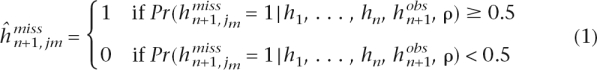where ρ is a given vector of recombination rates (which are estimated following the approach in McVean et al. (2002).

In the context of the tagging SNP selection problem, the (n + 1)th haplotype h_n+1 corresponds to a haplotype from a new data set, different from the one we use to choose the tags. The missing components correspond to the non-tagging SNPs, the observed components to tagging SNPs, and h₁, . . . , h_n correspond to the haplotypes in the training set. For instance, h_n+1 could be a haplotype in a future disease association study in which individuals have been genotyped only at the tags positions. Such studies aim to uncover associations between genotypes and a particular disease. The genetic variation in untyped loci can then be predicted using the rule in equation 1 and previously genotyped data h₁, . . . , h_n (e.g., HapMap). In the following, we describe what motivates the development of new methods to choose tagging SNPs.

Motivation to new approaches that select tagging SNPs

Before setting out the optimization problem that motivates our tagging SNPs selection scheme, we introduce some notation. Consider n haplotypes h₁, . . . , h_n evaluated at S biallelic loci. Denote by h_i = (h_i1, . . . , h_iS) the ith haplotype and by D = {h₁, . . . , h_n} the set of n haplotypes. Assume that each haplotype h_i can be decomposed in two vectors h_i = (h^_iT,h^_iNT), where h^_iT corresponds to the components of the tagging SNPs in the ith haplotypes and h^_iNT corresponds to the components of the non-tagging SNPs. Accordingly, D_T = {h^_1T, . . . , } consists of the set of n haplotypes evaluated at the tagging SNPs and D_NT = {h^_1NT, . . . , h^_nNT} the same set of haplotypes evaluated at non-tagging SNPs.

There are various ways in which the tagging SNPs can be chosen. A natural choice is to select the SNPs that maximize our ability to predict the non-tags. In other words, one wants to find the set where

For a given probability model, if it were possible to find the exact solution for , then this would be a desirable tagging SNP set. Unfortunately, an exact solution for would imply selecting all subsets SNPs, which becomes computationally unfeasible for the situations of interest with current genomic data. For this reason, we will look also at other tagging SNP sets with desirable properties, but whose constructions are computationally tractable.

Another way to choose the tags is to identify the SNPs that appear to be redundant, i.e., the SNPs that find other SNPs from the data set with similar information for the model. A possible approach to select these tags could then be to use the value of the likelihood to measure the relevance of the SNPs in the model. For example, if one deletes or considers missing some of the SNPs from the data set and recomputes the likelihood of the data set without these SNPs, then one could argue that the set of SNPs that keeps the value of the incomplete likelihood as close as possible to the value of the full likelihood could approximate the desirable tag set.

More explicitly, consider the set that satisfies the following condition

or equivalently,

While there are other possible motivations for SNP selection, in this work we limit ourselves to the exploration of the possibilities mentioned above.

We describe algorithms that find the set of tagging SNPs that attempts to capture the properties of and in the Supplemental material.

In the following we present the results of comparing these two approaches with ldSelect for selecting tagging SNPs.

Results

It has been suggested that the populations genotyped in the HapMap project may serve as reference populations for the selection of tagging SNPs in association studies. In addition to surveying variation genome-wide, the HapMap Project focused on 10 ENCODE regions for comprehensive genotyping as part of an in-depth study of human genetic variation. The regions were chosen to represent a range of conservation with the mouse genome and of gene density according to the strata identified during the ENCODE target selection process.

We measure the performance of our approach and compare it with ldSelect in the 10 ENCODE regions, which are each roughly 500 kb in length. Individuals from three populations were genotyped: 60 unrelated Europeans from Utah (CEU), 60 unrelated Africans from Nigeria (YRI), and 89 unrelated Asians (Han Chinese [HCB] and Japanese from Tokyo [JPT]). We consider only common SNPs within each population.

The comparison of the three algorithms tries to assess the performance of a set of tagging SNPs in a future association study by randomly assigning haplotypes from each of the three populations into equally sized training and test data sets. The training data set is used to perform the tagging SNP selection, while the test data set is not used to define the tagging SNPs, and thus is a proxy for the the genotypes obtained in the future study.

We measure the performance of the various algorithms using three criteria: proportion of non-tagging SNPs “captured,” misclassification rate, and the Brier score (Brier 1950).

Misclassification is an overall measure that is independent of the MAF of the SNPs. In the context of the tagging SNP selection problem, misclassification is the number of mismatches between the predicted non-tags and their actual values. Statistically, it is also an appealing quantity. It is a well-known statistical procedure to use an independent data set, different from the one used to estimate the parameters of a probabilistic model, to assess the performance of the model. In this context, the performance of a model refers to the ability of the model to predict a response variable. Specifically, it is desirable to minimize the expected prediction error E(L(Y, f(X; ))). Here Y denotes the response variable, X a set of covariates, and L the loss function, which is usually the squared error loss for continuous response variables and the 0–1 loss when the response variable is categorical, and f is a rule that links the response variable with the covariates and the parameters estimated with the data, . Assessing the performance or prediction error of a model using the same data with which the parameters of the model were estimated does not give an accurate estimate of the performance. Usually the prediction error can be dropped to zero by increasing the model complexity. A model with prediction error equal to zero is unrealistic and captures mainly features that are specific to the data used to build the model and will typically generalize poorly to other data sets (see Hastie et al. 2001 for more details).

In the context of tagging SNPs selection, for a fixed number of tags, we want to find the set of SNPs that minimize the expected prediction error when the 0–1 loss is considered and all non-tagging SNPs are predicted. By mimicking the statistical procedure mentioned in the above paragraph, we estimated the expected prediction error using an independent data set from the one used to choose the tagging SNPs. Misclassification rate is an estimate of the expected future prediction error of a model when a 0–1 loss of function is considered.

The Brier score is similar to the mean squared error (MSE), measuring the difference between the prediction probability of an event and its occurrence, expressed as 0 or 1 depending on whether a particular allele has occurred or not. It is also independent of the MAF of the SNPs.

Henceforth, we say that a non-tagging SNP is “captured” if the prediction of the non-tag has r² > 0.8 with the actual value of the non-tag in the test data set. Recall that by using the rule given by equation 1 and we can predict every non-tagging SNP. Therefore, for each non-tagging SNP, there is a predicted SNP that represents our “best” guess for that SNP. In a similar way, the “best” guess for each non-tag in the test data that ldSelect provides is the tag in the test data with which the non-tag has the highest r² value. The proportion of SNPs captured is given by the sum of the number of tagging SNPs and the number of non-tags captured divided by the total number of SNPs. Misclassification, for each SNP, is computed as the number of mismatches between the true SNP and its predicted SNP. The overall misclassification rate is given by the sum of the misclassifications given by each non-tag divided by the total number of SNPs and the total number of haplotypes in the test data. If the probabilities in the rule given by equation 1 are used to make the predictions, the Brier score is computed in the following way:

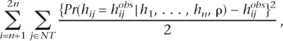where NT corresponds to the set of non-tagging SNPs and the sum is over the haplotypes in test data.

If, instead, we use ldSelect to predict the non-tags, then we replace the probability Pr(h_ij = h^_ijobs|h₁, . . . , h_n, ρ) in the above expression by either 1 or 0 depending on the value of the tag, evaluated at haplotype j, that has the highest r² value with the non-tag that we are trying to predict. In this case, the Brier score is proportional to the misclassification rate.

Generalization performance

It is well recognized that point estimators of r² have a high sampling variance (e.g., Ewen 1979) and therefore might indicate that one SNP captures another, when in fact it does not. Carlson et al. (2004) used simulated data to empirically test the reliability of the proportion of SNPs captured using r² values and different thresholds and concluded that thresholds >0.5 appear to yield more reliable results for the particular sample size that they used. We use ldSelect on the training set to choose the tags, using a cutoff of 0.8, and then assess its performance in capturing variation in the test data set.

We stopped the ldSelect algorithm after 50 and 100 SNPs were selected as tagging SNPs and measured the percentage of SNPs captured by these sets of SNPs and compared it with what is expected from training data (Table 1, first 6 rows). For example, with 50 tags, ldSelect tags capture 84% of the total number of SNPs in the combined Asian populations. When the same SNPs are considered in test data, 73% of the SNPs are captured. We note that regardless of the number of tagging SNPs chosen, when considering a new data set, ∼12% of the SNPs captured in training data are not captured in a new data set. Note also that the African population (YRI) requires more SNPs to capture the same proportion on non-tags than the European (CEU) or combined Asian populations (JPT+HCB). This agrees well with the evidence for slightly higher genetic diversity in the African populations, a fact that has been taken as evidence for the “out of Africa” model (see, e.g., Reich et al. 2001).

Table 1.

Proportion of SNPs captured averaged over the 10 ENCODE regions and 10 training-test splits

The numbers in parentheses correspond to the standard error.

ldSelect tagging SNPs vs. ldSelect tagging SNPs together with a model

To assess whether we could gain information from a probabilistic model in capturing non-tagging SNPs, we use the same set of tagging SNPs that ldSelect finds to predict all SNPs outside of the tagging SNP set using the Li and Stephens (2003) likelihood as explained above. In this case, the tagging SNPs correspond to the observed components of the haplotype and the remaining SNPs correspond to the missing components. The missing components are predicted using the rule given by equation 1. We estimate the r² value between all SNPs outside of the tagging SNP set with their predicted values using test data.

The difference in the percentage of SNPs captured by ldSelect compared with the ones captured by predicting the non-tags using the Li and Stephens’ (2003) model is more noticeable when the number of tagging SNPs is smaller. Using the Li and Stephens’ (2003) model to predict non-tagging SNPs allows an increase of 11% in the captured SNPs in the YRI population when 50 and 100 SNPs are in the tagging SNP set and between 6% and 8% in the JPT+HCB and CEU populations for the same number of SNPs (Table 1). If resources are limited in an association study and one is restricted to genotyping only a small fraction of the SNPs, then the gain obtained by predicting SNPs based on the Li and Stephens’ (2003) model can be important.

Another way to assess the performance of the tagging SNPs is the misclassification rate, which reflects the overall error in prediction. The results for ldSelect in training and test data are shown in Table 2. The performance of tagging SNPs chosen by ldSelect between training and testing data decreases slightly, and again we can see that the gain is about 2%–4% when we predict the non-tags using LS.

Table 2.

Misclassification rate averaged over the 10 ENCODE regions and 10 training-test splits

The numbers in parentheses correspond to the standard error.

We have described a way in which we can capture more of the genetic variation by using the tagging SNPs chosen by ldSelect algorithm and predicting the non-tagging SNPs using the Li and Stephens’ (2003) model. The next section shows that if we additionally use the Li and Stephens’ (2003) model to choose the tags as described above, we are able to capture even more of the genetic variation.

Performance of ldSelect tags vs performance of and

We now compare the performance of the sets and of tagging SNPs that approximate the exact solution of and , respectively. These sets of tags are used to predict the non-tags using the rule given by equation 1. We use 10 training-test splits of the data to provide error estimates in the evaluation of performance.

The results of the Brier scores, misclassification, and proportion of SNPs captured, averaged over the 10 ENCODE regions and the 10 training-test splits, are shown in Tables 3, 2, and 1, respectively, for , and ldSelect tags. Table 1 shows a slight improvement of 1%–3% in the proportion of SNPs captured by the tags when these have been chosen, using compared with the performance when the tags have been chosen using ldSelect. The Brier score is shown for , and ldSelect in Table 3. Our approach using shows the smaller Brier scores in the three populations, which reflects better confidence in the predictions. Misclassification remains roughly the same in the three algorithms (Table 2).

Table 3.

Brier score when tagLS and ldSelect tags (respectively) are used and the non-tags are predicted using the rule given by equation 1 (L+S)

The numbers in parentheses correspond to the standard error.

Another way of assessing how much of the genetic variation is captured by predicting the non-tags is through a statistical test that computes the non-random association between the predicted non-tag and its true value. In particular, the P-values of such tests provide a measure of how likely it is to observe data at least as extreme as the sample data when the predicted non-tag and its true value are independent. In the following section we applied one such test to our predicted data.

Fisher’s exact test

Fisher’s exact test is a statistical test used to determine whether there are nonrandom associations between two categorical variables (see Agresti 1990 for details). When one or more of the expected numbers in a 2 × 2 table is less than five, and when the overall sample size is small, it is commonly believed that Fisher’s test remains a reliable test. We consider three sets of 50 tags given by ldSelect, , and , and assume one by one that each non-tag is the causal SNP. We want to test whether one would be able to capture this causal SNP in individuals where one has observed the tags and has a predicted estimate of the causal SNPs. We perform Fisher’s exact test between each non-tag SNP and its predicted SNP obtained using the rule given by equation 1 in test data in the 10 ENCODE regions. Figure 1 shows the sorted P-values obtained in this test that we denote by test1. Each panel contains the P-values of a different population. From left to right, the panels contain the P-values in the European population (CEU), in the combined Asian populations (JPT+HCB), and in the African population (YRI), respectively. The black lines (continuous line), green (dotted), and blue (dot-line) represent the sorted P-values for the test performed using ldSelect tags, and , respectively. Consistently, the P-values are smaller in the three populations when tags have been used. does slightly worse than the other two sets in the CEU population, and in the YRI population, the performance of ldSelect is slightly lower than for the other two sets.

Figure 1.

Sorted P-values of Fisher’s exact test (test1) in the three populations CEU (left), JPT+HCB (middle), and YRI (right) evaluated in test data in the 10 ENCODE regions.

To compute the P-values, we first calculate the probability of the 2×2 table given a particular row and column sums in the following way:

where C_i and R_j denote the row and column sums, respectively, and N = ∑²_i=1 ∑²_j=1 a_ij = ∑_i C_i = ∑_j R_j = number of haplotypes in the test data. Then the P-value of test1 is the sum of the probabilities of all of the possible tables of non-negative integers, consistent with the row and column sums that have probability less than or equal to P_obs.

To assess the prediction performance of the ldSelect tags when the probabilistic model is not used to predict the non-tags, we compute a second test denoted by test2. Again, each non-tag is assumed to be the causal SNP one by one. To compute the P-values of test2 for each causal SNP, we first calculate the P-value of Fisher’s test between the causal SNP and each tag and obtain the minimum value (denoted ). Then, we permute the causal SNP status 1000 times, and each time we compute the minimum P-value of Fisher’s test over all of the tags and count how many times this minimum value is smaller than . The P-value for test2 is then this count divided by 1000. In Figure 1 the sorted P-values are depicted by the red dashed lines in the three panels. It can be seen that the P-values for test2 are considerably higher than the P-values for test1. This fact illustrates another advantage of the method that predicts the non-tags using an informative probabilistic model as opposed to just using the tags to capture the genetic variation of the region.

Rare SNPs

Rare SNPs are in general difficult to be captured by other SNPs. It is therefore of interest to assess the performance of the various set of tags considered here on rare SNPs. To assess the performance of these methods on rare SNPs, we compute the frequency of captured and uncaptured SNPs for values of the frequency of the MAF between 2 and 7. The results are illustrated in Figure 1 in the Supplemental material, in which we plot a set of barplots above the frequency of the MAF. These barplots are made up of eight bars that correspond to the following: The first two bars correspond to the number of non-tags captured by tags and our method for predicting non-tags, followed by the number of non-tags uncaptured; the third and fourth correspond to the number of non-tags captured by tags and our method for predicting non-tags, followed by the number of non-tags uncaptured; the fifth and sixth bars correspond to the number of non-tags captured by ldSelect tags and our method for predicting non-tags, followed by the number of non-tags uncaptured; the last two columns correspond to the the number of non-tags captured by ldSelect tags, followed by the number of non-tags uncaptured. The upper panel shows the performance of the algorithms using 50 tags and the lower panel the performance of the algorithms using 100 tags. Note that each method chooses a different set of tags; therefore, the sums of the totals in the first and second bars, second and third, forth and fifth, and sixth and eighth should be similar but not necessarily equal.

It is apparent from Figure 1 (in Supplemental material) that pure ldSelect tags are consistently worst performers. On the other hand, the other three methods perform roughly similarly. We conclude from this exercise that using our method for predicting non-tags is the most important factor in increasing the capture of rare SNPs by the tags, with the actual algorithm used to choose the tags being of lesser importance.

Is there a better tagging SNP set?

How much better can a tagging SNP set perform if one is not constrained by computational costs? Is there another tagging SNP set that could capture significantly more genetic variation? In this section we briefly address these questions. We argue using a data set where we are not constrained by computational feasibility that a more desirable set of tags, maxT, is one that maximizes the predictive probability of the non-tags given the tags and some reference data set. As described above, our set attempts to approximate this set.

In order to illustrate the performance of the set maxT, we consider three genes with few SNPs in the CEU population of HapMap data, in which it is computationally feasible to look at all possible sets of tags of a given size. We compute the Li and Stephens (2003) likelihood at each set of tags using training data and choose the set that maximizes the probability of the non-tags given the tags and some reference data D, Pr(D_NT|D_T,D) in the notation of the previous section (or, equivalently, we choose the set of tags that minimizes the probability of the tags Pr(D_T,D) together with D. In this case, we consider D to be a subset of the haplotypes from training data (in our experiments we use a third of the haplotype of training data for this purpose) and evaluate the remaining haplotype only at the components where the tags are and compute the likelihood Pr(h₁, . . . , h_n1, + 1, . . . , ). We then evaluate the performance of the tags in the test data.

The results are shown in Table 4. In column 1 we show the three genes considered. ADD1 is a gene in chromosome 4 with 86,180 bp length, and contains 20 SNPs in HapMap data, ADD2 is located in chromosome 2 with 106,067 bp length with 31 SNPs, and WNK1 is in chromosome 12 with 155,227 bp length with 46 SNPs in HapMap data. In columns 3–5 we show the performance of ldSelect, and maxT, respectively, using the number of tags indicated in column 2. The performance is assessed by the proportion of non-tags that are captured by the tags. It is apparent that overall maxT is a better performer than either of T₁ or ldSelect, showing that it is indeed a more desirable set of tags when computational limitations are not an issue. Note that maxT is not always the best performer, but this is to be expected due to the intrinsic uncertainty of predicting tags in a set different from the training one.

Table 4.

Proportion of SNPs captured by ldSelect, , and maxT (columns 3–5) for the genes indicated in column 1 when using the number of tags indicated in column 2

It is apparent that maxT is a better performer in the case that all subsets of a given size can be explored.

Discussion

We have proposed a method to predict non-tags using the tags and the PAC likelihood of the Li and Stephens’ (2003) model. The PAC likelihood fits haplotype data that incorporates genetic factors such as distance between SNPs, recombination rates, and probability of mutations. When the tagging SNPs have been selected based on the ldSelect algorithm, we show that by predicting the non-tagging SNPs with our method we can capture significantly more of the genetic variation in a region than by capturing the variation based solely on the tagging SNPs and a pairwise LD measure as prescribed by ldSelect. Our novel method suggests a way to use the markers in order to capture more genetic variation.

We also developed new algorithms to select tagging SNPs that include the PAC likelihood of Li and Stephens (2003) in the selection process itself. We measure the performance of two approaches for selecting tags together with the method for predicting non-tags and compare it with the performance of ldSelect using three criteria: Brier score, misclassification, and proportion of non-tagging SNPs captured in independent data, i.e., different haplotype data from the one used to choose the tagging SNPs. In this way, we assess the performance of the algorithms in future association studies. We show that the set of tags always outperform ldSelect based on three criteria, and the set of tags outperforms ldSelect according to the Brier score, but ldSelect performs better when the number of SNPs captured is measured and 50 tags have been used to predict the non-tags.

The ability to predict the non-tags offers several advantages. The most obvious one is that it provides an extra SNP, beside the tagging SNPs, with which we can test for association with the phenotype. Additionally, it provides an estimate of the probabilities with which the prediction of the non-tags are made that reflects the confidence of the probabilistic model. Another advantage occurs when independent sets are considered to choose the tagging SNPs and to genotype individuals for an association study. For example, if the reference data set comes from an older population with more genetic variation than the population considered in the association study, then it might happen that a SNP appears to be monomorphic in a group of individuals considered for an association study. A monomorphic SNP in test data is not able to find any surrogate SNP in the tagging SNP set, because the r² value between itself and any other SNP does not exist unless the other SNP considered is also monomorphic, in which case, r² = 1. Our approach has the advantage that a monomorphic SNP can be predicted perfectly, whereas methods based on r² will never be able to capture such a SNP.

We computed P-values for Fisher’s exact test (test1) between each non-tag and its predicted SNP, assuming that all non-tags are one by one the causal SNPs. We also computed the minimum P-values for Fisher’s exact test between each non-tag and the tags (test2). We show that there are a considerably larger proportion of smaller P-values in test1 compared with test2, reflecting an advantage of the probabilistic model in capturing genetic variation.

Our methods were developed favoring ease of computation and fast implementation rather than exact calculations, which are unfeasible for large data sets such as current genomic data. There are still possible directions that could lead to improvement of the methods proposed. One possibility is to optimize the algorithm that searches for the best tagging SNP set, i.e., finding a better approximation to max_TPr(D_NT|D_T). Another possibility is to do the prediction of the non-tags taking into account the dependence between the SNPs, which we are not considering in this work. These possibilities will be explored in future work.

The code of these algorithms is written in Perl and C++ programming languages and is available at http://www.statistik.lmu.de/~eyheram/software/genecap/.

References

- Agresti A. Categorical data analysis. John Wiley & Sons; New York: 1990. [Google Scholar]
- Brier G.W. Verification of forecasts expressed in terms of probability. Mon. Weather Rev. 1950;78:1–3. [Google Scholar]
- Carlson C.S., Eberle M.A., Rieder M.J., Yi Q., Kruglyak L., Nickerson D.A., Eberle M.A., Rieder M.J., Yi Q., Kruglyak L., Nickerson D.A., Rieder M.J., Yi Q., Kruglyak L., Nickerson D.A., Yi Q., Kruglyak L., Nickerson D.A., Kruglyak L., Nickerson D.A., Nickerson D.A. Selecting a maximally informative set of single-nucleotide polymorphisms for association analyses using linkage disequilibrium. Am. J. Hum. Genet. 2004;74:106–120. doi: 10.1086/381000. [DOI] [PMC free article] [PubMed] [Google Scholar]
- Chapman J.M., Cooper J.D., Todd J.A., Clayton D.G., Cooper J.D., Todd J.A., Clayton D.G., Todd J.A., Clayton D.G., Clayton D.G. Detecting disease associations due to linkage disequilibrium using haplotype tags: A class of tests and the determinants of statistical power. Hum. Hered. 2003;56:18–31. doi: 10.1159/000073729. [DOI] [PubMed] [Google Scholar]
- Clayton D. Choosing a set of haplotype tagging SNPs from a larger set of diallelic loci. http://www.nature.com/ng/journal/v29/n2/extref/ng1001-233-S10.pdf 2001 [Google Scholar]
- deBakker P.I., Yelensky R., Pe’er I., Gabriel S.B., Daly M.J., Altshuler D., Yelensky R., Pe’er I., Gabriel S.B., Daly M.J., Altshuler D., Pe’er I., Gabriel S.B., Daly M.J., Altshuler D., Gabriel S.B., Daly M.J., Altshuler D., Daly M.J., Altshuler D., Altshuler D. Efficiency and power in genetic association studies. Nat. Genet. 2005;37:1217–1223. doi: 10.1038/ng1669. [DOI] [PubMed] [Google Scholar]
- Devlin B., Risch N., Risch N. A comparison of linkage disequilibrium measures for fine-scale mapping. Genomics. 1995;29:311–322. doi: 10.1006/geno.1995.9003. [DOI] [PubMed] [Google Scholar]
- Ewen W. Mathematical population genetics. Springer Verlag; New York: 1979. [Google Scholar]
- Goldstein D.B., Ahmadi K.R., Weale M.E., Wood N.W., Ahmadi K.R., Weale M.E., Wood N.W., Weale M.E., Wood N.W., Wood N.W. Genome scans and candidate gene approaches in the study of common diseases and variable drug responses. Trends Genet. 2003;19:615–622. doi: 10.1016/j.tig.2003.09.006. [DOI] [PubMed] [Google Scholar]
- The International HapMap Consortium, The international hapmap project. Nature. 2003;426:789–796. doi: 10.1038/nature02168. [DOI] [PubMed] [Google Scholar]
- Hastie T.J., Tibshirani R.J., Friedman J., Tibshirani R.J., Friedman J., Friedman J. The elements of statistical learning. Data mining inference and prediction. Springer-Verlag; New York: 2001. [Google Scholar]
- Hu X., Schrodi S.J., Ross D.A., Cargill M., Schrodi S.J., Ross D.A., Cargill M., Ross D.A., Cargill M., Cargill M. Selecting tagging SNPs for association studies using power calculations from genotype data. Hum. Hered. 2004;57:156–170. doi: 10.1159/000079246. [DOI] [PubMed] [Google Scholar]
- Johnson G.C.L., Esposito L., Barrat B.J., Smith A., Heward J., Di Genova G., Ueda H., Cordell H., Eaves I., Dudbridge F., Esposito L., Barrat B.J., Smith A., Heward J., Di Genova G., Ueda H., Cordell H., Eaves I., Dudbridge F., Barrat B.J., Smith A., Heward J., Di Genova G., Ueda H., Cordell H., Eaves I., Dudbridge F., Smith A., Heward J., Di Genova G., Ueda H., Cordell H., Eaves I., Dudbridge F., Heward J., Di Genova G., Ueda H., Cordell H., Eaves I., Dudbridge F., Di Genova G., Ueda H., Cordell H., Eaves I., Dudbridge F., Ueda H., Cordell H., Eaves I., Dudbridge F., Cordell H., Eaves I., Dudbridge F., Eaves I., Dudbridge F., Dudbridge F., et al. Haplotype tagging for the identification of common disease genes. Nat. Genet. 2001;29:233–237. doi: 10.1038/ng1001-233. [DOI] [PubMed] [Google Scholar]
- Kruglyak L. Prospects for whiole-genome linkage disequilibrium mapping of common disease genes. Nat. Genet. 1999;22:139–144. doi: 10.1038/9642. [DOI] [PubMed] [Google Scholar]
- Li N., Stephens M., Stephens M. Modelling Linkage Disequilibrium, and identifying recombination hotspots using SNP data. Genetics. 2003;165:2213–2233. doi: 10.1093/genetics/165.4.2213. [DOI] [PMC free article] [PubMed] [Google Scholar]
- McCarroll S., Hadnott T., Perry G., Sabeti P., Zody M., Barret J., Dallaire S., Gabriel S., Lee C., Daly M., Hadnott T., Perry G., Sabeti P., Zody M., Barret J., Dallaire S., Gabriel S., Lee C., Daly M., Perry G., Sabeti P., Zody M., Barret J., Dallaire S., Gabriel S., Lee C., Daly M., Sabeti P., Zody M., Barret J., Dallaire S., Gabriel S., Lee C., Daly M., Zody M., Barret J., Dallaire S., Gabriel S., Lee C., Daly M., Barret J., Dallaire S., Gabriel S., Lee C., Daly M., Dallaire S., Gabriel S., Lee C., Daly M., Gabriel S., Lee C., Daly M., Lee C., Daly M., Daly M., et al. Common deletion polymorphisms in the human genome. Nat. Genet. 2005;38:86–92. doi: 10.1038/ng1696. [DOI] [PubMed] [Google Scholar]
- McVean G., Awadalla P., Fearnhead P., Awadalla P., Fearnhead P., Fearnhead P. A coalescent-based method for detecting and estimating recombination from gene sequences. Genetics. 2002;160:1231–1241. doi: 10.1093/genetics/160.3.1231. [DOI] [PMC free article] [PubMed] [Google Scholar]
- Pritchard J.K., Przeworski M., Przeworski M. Linkage disequilibrium in humans: Models and data. Am. J. Hum. Genet. 2001;69:1–14. doi: 10.1086/321275. [DOI] [PMC free article] [PubMed] [Google Scholar]
- Reich D.E., Cargill M., Bolk S., Ireland J., Sabeti P.C., Richter D.J., Lavery T., Kouyoumjian R., Farhadian S.F., Ward R., Cargill M., Bolk S., Ireland J., Sabeti P.C., Richter D.J., Lavery T., Kouyoumjian R., Farhadian S.F., Ward R., Bolk S., Ireland J., Sabeti P.C., Richter D.J., Lavery T., Kouyoumjian R., Farhadian S.F., Ward R., Ireland J., Sabeti P.C., Richter D.J., Lavery T., Kouyoumjian R., Farhadian S.F., Ward R., Sabeti P.C., Richter D.J., Lavery T., Kouyoumjian R., Farhadian S.F., Ward R., Richter D.J., Lavery T., Kouyoumjian R., Farhadian S.F., Ward R., Lavery T., Kouyoumjian R., Farhadian S.F., Ward R., Kouyoumjian R., Farhadian S.F., Ward R., Farhadian S.F., Ward R., Ward R., et al. Linkage disequilibrium in the human genome. Nature. 2001;411:199–204. doi: 10.1038/35075590. [DOI] [PubMed] [Google Scholar]
- Schork N.J. Power calculations for genetic association studies using estimated probability distributions. Am. J. Hum. Genet. 2002;70:1480–1489. doi: 10.1086/340788. [DOI] [PMC free article] [PubMed] [Google Scholar]
- Sebastiani P., Lazarus S.W., Kunkel L.M., Kohane I.S., Ramoni M., Lazarus S.W., Kunkel L.M., Kohane I.S., Ramoni M., Kunkel L.M., Kohane I.S., Ramoni M., Kohane I.S., Ramoni M., Ramoni M. Minimal haplotype tagging. Proc. Natl. Acad. Sci. 2003;100:9900–9905. doi: 10.1073/pnas.1633613100. [DOI] [PMC free article] [PubMed] [Google Scholar]
- Wang W.Y.S., Barratt B.J., Clayton D.G., Todd J.A., Barratt B.J., Clayton D.G., Todd J.A., Clayton D.G., Todd J.A., Todd J.A. Genome-wide association studies: Theoretical and practical concerns. Nat. Rev. Genet. 2005;6:109–118. doi: 10.1038/nrg1522. [DOI] [PubMed] [Google Scholar]
- Weale M., Depondt C., MacDonald S., Smith A., Lai P., Shorvon S., Wood N., Goldstein D., Depondt C., MacDonald S., Smith A., Lai P., Shorvon S., Wood N., Goldstein D., MacDonald S., Smith A., Lai P., Shorvon S., Wood N., Goldstein D., Smith A., Lai P., Shorvon S., Wood N., Goldstein D., Lai P., Shorvon S., Wood N., Goldstein D., Shorvon S., Wood N., Goldstein D., Wood N., Goldstein D., Goldstein D. Selection and evaluation of tagging SNPs in the neuronal-sodium-channel gene mapping. Am. J. Hum. Genet. 2003;73:551–565. doi: 10.1086/378098. [DOI] [PMC free article] [PubMed] [Google Scholar]
- Zhang K., Qin Z., Liu J., Chen T., Waterman M., Sun F., Qin Z., Liu J., Chen T., Waterman M., Sun F., Liu J., Chen T., Waterman M., Sun F., Chen T., Waterman M., Sun F., Waterman M., Sun F., Sun F. Haplotype block partitioning and tag SNP selection using genotype data and their applications to association studies. Genome Res. 2004;14:908–916. doi: 10.1101/gr.1837404. [DOI] [PMC free article] [PubMed] [Google Scholar]
- Zondervan K.T., Cardon L.R., Cardon L.R. The complex interplay among factors that influence allelic association. Nat. Rev. Genet. 2004;5:89–100. doi: 10.1038/nrg1270. [DOI] [PubMed] [Google Scholar]