Theory of femtosecond stimulated Raman spectroscopy

Abstract

Femtosecond broadband stimulated Raman spectroscopy (FSRS) is a new technique that produces high-resolution (time-resolved) vibrational spectra from either the ground or excited electronic states of molecules, free from background fluorescence. FSRS uses simultaneously a narrow bandwidth ∼1 – 3 ps Raman pump pulse with a continuum ∼30– 50 fs Stokes probe pulse to produce sharp Raman gains, at positions corresponding to vibrational transitions in the sample, riding on top of the continuum Stokes probe spectrum. When FSRS is preceded by a femtosecond actinic pump pulse that initiates the photochemistry of interest, time-resolved Raman spectroscopy can be carried out. We present two theoretical approaches to FSRS: one is based on a coupling of Raman pump and probe light waves with the vibrations in the medium, and another is a quantum-mechanical description. The latter approach is used to discuss the conditions of applicability and limitations of the coupled-wave description. Extension of the quantum-mechanical description to the case where the Raman pump beam is on resonance with an excited electronic state, as well as when FSRS is used to probe a nonstationary vibrational wave packet prepared by an actinic pump pulse, is also discussed.

I. INTRODUCTION

Raman spectroscopy is a powerful analytical and vibrational structure elucidation technique widely used in chemical, biological, and time-resolved studies.^1-3 However, most molecules and associated impurities tend to produce background fluorescence that can easily overwhelm the relatively weak Raman signal, making it difficult to exploit the technique routinely, especially for time-resolved studies. The advent of commonly available femtosecond lasers has catalyzed interest in time-resolved vibrational spectroscopy techniques to reveal the structural changes underlying ultrafast chemical and biological reaction processes. Two fundamental obstacles are encountered.

(1) The difficulty of generating ultrafast laser pulses throughout the midinfrared for direct IR absorption. Direct IR probing techniques have been generally limited to ∼200 fs time resolution in a narrow (∼200 cm⁻¹) spectral region.

(2) The pulse duration/bandwidth transform limit in Raman spectroscopy. A full Raman vibrational spectrum over a ∼3000 cm⁻¹ window can be obtained, but pulse durations >0.7 ps are necessary to achieve acceptable spectral resolution.

In conventional, spontaneous Raman spectroscopy, a coherent pump beam at ω_p is incident on a sample, and Stokes ω_s and anti-Stokes ω_as photons are generated into the zero-point radiation field.^4,5 However, when two optical fields, a coherent Raman pump beam at ω_p and a Stokes probe beam ω_s (or an anti-Stokes probe beam ω_as), are incident on a sample that contains a molecular vibration ω₀=ω_p−ω_s (or ω₀=ω_as−ω_p), coherent stimulated Raman light, a nonlinear effect,^6,7 shows up as gain at ω_s (or ω_as), with a much larger scattering cross section that is proportional to the spectral photon flux of the Stokes (or anti-Stokes) field. Stimulated Raman scattering using an intense coherent pump beam was first observed by Woodbury and Ng,⁸ and explained by Eckhardt et al. ⁹

To overcome the difficulties and limitations of conventional Raman spectroscopy mentioned above, for both cw and time-resolved studies with ultrashort pulses, a new technique, femtosecond stimulated Raman spectroscopy (FSRS), has been developed.^10-13 It produces high-quality vibrational spectra free from background fluorescence and permits rapid collection of high-resolution vibrational spectra on the femtosecond time scale of both ground and excited electronic state species. FSRS uses two NIR pulses:^10-12 a narrow bandwidth (1–3 ps, ∼5–15 cm⁻¹, 30–1500 nJ) Raman pump pulse centered at 795 nm, and a continuum Stokes probe pulse (30–50 fs, 830–960 nm, <20 nJ) to the red of the pump which provides Stokes fields covering vibrations in the range 450–2100 cm⁻¹. By tuning the wavelength of the pump pulse, the window for observing vibrations can be extended down to ∼200 cm⁻¹ and up to 2600 cm⁻¹. When both pump and probe pulses are incident on the sample simultaneously, sharp Raman gain features are observed on top of the continuum probe spectrum due to stimulated Raman transitions, as exemplified in Fig. 1(a) for cyclohexane. The sharp features are fundamental Raman transitions of different vibrational modes of the sample. By taking the ratio of pump-on and pump-off probe spectra, i.e., the transmittance (I/I ₀), a conventional-looking Raman spectrum is obtained, as shown in Fig. 1(b). The spectral resolution of the gain profile is limited by the duration of the Raman pump, the natural vibrational linewidth of the system, and the resolution of the spectrograph (currently <8cm⁻¹).

FIG. 1.

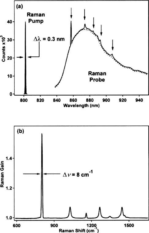
(a) The spectra of Raman pump and Stokes probe pulses for a typical FSRS experiment on cyclohexane. The pump-off probe spectrum is shown as the dotted line. With the pump-on, the Raman gain peaks from the cyclohexane are clearly visible in the output Stokes probe spectrum (solid). (b) The ratio of the Stokes probe spectrum with and without the Raman pump gives the Raman gain spectrum.

The theory of Raman spectroscopy has a long history,⁵ encompassing both classical¹⁴ and quantum¹⁵ approaches tracing back to the beginnings of quantum theory. The quantum-mechanical Kramers-Heisenberg-Dirac scattering theory¹⁵ can account for both spontaneous and stimulated Raman scattering with narrow bandwidth cw radiation, and typically a sum-over-states, time-independent approach is used. Shen and Bloembergen¹⁶ have also provided a classical coupled-wave description of stimulated Raman scattering with cw radiation. While the narrow bandwidth Raman pump pulse in FSRS can, to a good approximation, be taken to be cw, the continuum femtosecond Stokes probe pulse clearly cannot be, and so the existing theories for stimulated Raman scattering which are geared towards cw pump and probe pulses need to be reexamined and modified.

The purpose of this paper is to present and compare the classical coupled wave theory with the quantum theory for FSRS, and to explain the peak position and the width of the observed Raman gain signal in FSRS for the situation where the peaks of the Gaussian Raman pump and Stokes probe fields coincide. In Sec. II, the coupled-wave description of stimulated Raman scattering for cw radiation¹⁶ is extended to FSRS, and the quantum theory of FSRS using a time-dependent density matrix approach via the nonlinear third-order polarization is also presented. In Sec. III we discuss (a) the conditions of applicability and limitations of the coupled-wave description, (b) the extension of the quantum theory of FSRS to the case when the pump is on resonance with an excited electronic state, and (c) when FSRS is used to probe a nonstationary vibrational wave packet prepared by an actinic pump pulse.

II. THEORY

A. Coupled-wave description of FSRS

The physical picture of light interacting with a medium is the following: An intense electric field $\overrightarrow{E}(\overrightarrow{r},t)$ induces a nonlinear response in the medium, described by the polarization $\overrightarrow{P}(\overrightarrow{r},t)$ as a function of the electric field $\overrightarrow{E}(\overrightarrow{r},t)$, known as the constitutive equation. The reacting medium modifies the optical fields in a nonlinear way as they propagate through the medium, a process described by the Maxwell equations.

The medium is taken to be a collection of oscillators with vibrational coordinate Q, and we consider just one vibrational mode here of angular frequency ω₀. The Lagrangian density for the light coupled to the vibrations is given by

$$L=L_{\mathit{rad}}+L_{\mathit{vib}}+L_{\mathrm{int}},$$ (1)

where the Lagrangian for the radiation comprising the total transverse electric field $\overrightarrow{E}$ and magnetic induction $\overrightarrow{B}$ is

$$L_{\mathit{rad}}=\frac{1}{2}(\mid \overrightarrow{E}{\mid }^2-\mid \overrightarrow{B}{\mid }^2),$$ (2)

the Lagrangian for the vibration is

$$L_{\mathit{vib}}=N\{\frac{1}{2}{\dot{Q}}^2-\frac{1}{2}{\omega }_0^2{Q}^2\},$$ (3)

where N is the number of oscillators per unit volume, and the interaction of the light with the medium is given by

$$L_{\mathrm{int}}=-N(-\overrightarrow{P}\cdot \overrightarrow{E})=N\alpha :\overrightarrow{E}\overrightarrow{E},$$ (4)

where we have invoked the Placzek model¹⁴ for the polarization of the oscillator, $\overrightarrow{P}(\overrightarrow{r},t)=\alpha \cdot \overrightarrow{E}(\overrightarrow{r},t)$, where $\overrightarrow{r}$ is a macroscopic coordinate through the medium, and the polarizability α (a molecular property) can, furthermore, be expanded in a Taylor series in the vibrational coordinate Q,

$$\alpha \approx {\alpha }_0+{\left(\frac{d\alpha }{dQ}\right)}_{0}Q+\cdots \equiv {\alpha }_0+{\alpha }_0^{\prime }Q+\cdots .$$ (5)

The Lagrange equation of motion,

$$\frac{\partial }{\partial t}\left(\frac{\partial L}{\partial \dot{Q}}\right)-\frac{\partial L}{\partial Q}=0$$ (6)

then yields the equation of motion for the vibration Q,

$$\frac{d^{2}Q}{d{t}^2}+2\gamma \frac{dQ}{dt}+{\omega }_0^{2}Q={\alpha }_0^{\prime }\mid \overrightarrow{E}(\stackrel{\rightharpoonup }{r},t){\mid }^2,$$ (7)

where we have added a phenomenological damping term 2γdQ/dt for the vibration which decays as e ^−γt. The damping constant γ would typically be given by $\gamma =T_Q^{-1}+T_{\mathit{pop}}^{-1}$, where T _Q is the vibrational dephasing time and T _pop is the lifetime of the transient species bearing the vibration.

The Maxwell equation (in Gaussian units)¹⁷ for the electric field is given by

$${\nabla }^2\overrightarrow{E}(\overrightarrow{r},t)-\frac{1}{c^2}\frac{{\partial }^2\overrightarrow{E}(\overrightarrow{r},t)}{\partial t^2}=\frac{4\pi N}{c^2}\frac{{\partial }^2\overrightarrow{P}(\overrightarrow{r},t)}{\partial t^2}.$$ (8)

This equation describes how the medium modifies the macroscopic field $\overrightarrow{E}(\overrightarrow{r},t)$. Henceforth, for convenience, we will assume that the light is linearly polarized and propagating along the z axis, and using the Placzek model above, the Maxwell equation becomes

$$\frac{{\partial }^{2}E(z,t)}{\partial z^2}-\frac{1}{c^2}\frac{{\partial }^{2}E(z,t)}{\partial t^2}\approx \frac{4\pi }{c^2}N{\alpha }_0^{\prime }\frac{{\partial }^2\left(QE(z,t)\right)}{\partial t^2},$$ (9)

where we have assumed that $N{\alpha }_0\ll 1$, which is generally true with N≈10²¹ cm⁻³ and α₀≈10⁻²⁴ cm³. Equations (7) and (9) are the central equations that can be used to describe stimulated Raman scattering. We first solve for Q(t) using Eq. (7) and the result is then used in the Maxwell equation (9) to solve for the output field E(z,t).

The total field in FSRS is a sum of a Raman pump field and a Stokes probe field,

$$E(z,t)=E_p(z,t)+E_s(z,t),$$ (10)

and we shall take the initial plane-polarized Raman pump and Stokes probe fields to act simultaneously on the sample and have Gaussian pulse envelopes as follows:

$$E_p(z,t)=E_p^0{e}^{-{(t-z∕c)}^2∕2{\tau }_p^2}{e}^{-i{\omega }_p(t-z∕c)},$$ (11)

$$E_s(z,t)=E_s^0{e}^{-{(t-z∕c)}^2∕2{\tau }_s^2}{e}^{-i{\omega }_s(t-z∕c)},$$ (12)

whose spectra (given by the Fourier transform ${\int }_{-\infty }^{\infty }\mathit{dt}{e}^{i\omega t\dots }$) are

$$E_p(z,\omega )=E_p^0\sqrt{2\pi }{\tau }_p{e}^{-{(\omega -{\omega }_p)}^2{\tau }_p^2∕2}{e}^{i\omega z∕c},$$ (13)

$$E_s(z,\omega )=E_s^0\sqrt{2\pi }{\tau }_s{e}^{-{(\omega -{\omega }_s)}^2{\tau }_s^2∕2}{e}^{i\omega z∕c}.$$ (14)

In the FSRS experiments of McCamant et al.,^10-12 the pump field E _p(z,t) is a 793 nm long pulse (τ_p∼1 – 3 ps) of narrow bandwidth (∼5–15 cm⁻¹), while the Stokes probe field E _s(z,t) is a 830–950 nm continuum ultrashort pulse (τ_s∼30–50 fs) covering stimulated Raman shifts of 500–2300 cm⁻¹. The pump pulse, in particular, can be considered to be very long compared to the vibrations with periods of 15–70 fs (500–2300 cm⁻¹), and so can even be considered as monochromatic. It is also possible experimentally to introduce a time–delay between the Raman pump and Stokes probe fields, and this will be taken up in a subsequent paper.¹⁸

Now, |E(z,t)|² would have four components, and the component $E_p(z,t)E_s^{\ast }(z,t)$ would possess the right frequency, $~e^{-i({\omega }_p-{\omega }_s)t}$, to exert a resonant forcing term and set in motion a coherent vibration, $Q~e^{-i{\omega }_{0}t}$, and Eq. (7) then becomes

$$\frac{d^{2}Q}{d{t}^2}+2\gamma \frac{dQ}{dt}+{\omega }_0^{2}Q={\alpha }_0^{\prime }{E}_p{E}_s^{\ast }.$$ (15)

Similarly, the component $E_p^{\ast }(z,t)E_s(z,t)$ would induce a coherent vibration $Q^{\ast }~e^{i{\omega }_{0}t}$. Using Eqs. (11) and (12) in Eq. (15), and defining t′=t−z/c, we obtain

$$\frac{d^{2}Q}{d{t}^2}+2\gamma \frac{dQ}{dt}+{\omega }_0^{2}Q=E_p^0{E_s^0}^{\ast }{\alpha }_0^{\prime }{e}^{-{t^{\prime }}^2∕2{\tau }^2-i({\omega }_p-{\omega }_s)t^{\prime }},$$ (16)

where we have defined $1∕{\tau }^2=1∕{\tau }_p^2+1∕{\tau }_s^2$. Clearly, the vibration is acted on by an impulsive force due to the coupled fields for a duration of order τ, which in the experiments of McCamant et al. ^10-12 corresponds to the ultrashort Stokes pulse duration, τ≈τ_s∼30–50 fs.

To solve Eq. (16) for the particular solution Q _ρ(z,t) we take a Fourier transform ${\int }_{-\infty }^{\infty }\mathit{dt}{e}^{i\omega t\dots }$ (note that it is with respect to t and not t′) and integrate by parts to remove the derivatives in t, to yield the solution in frequency space,

$$Q_{\rho }(z,\omega )=\frac{f\left(\omega \right)e^{i\omega z∕c}}{{\omega }_0^2-{\omega }^2-i2\gamma \omega }$$ (17)

with f(ω) given by

$$\begin{array}{cc}\hfill f\left(\omega \right)& ={\int }_{-\infty }^{\infty }{E}_p^0{E_s^0}^{\ast }{\alpha }_0^{\prime }{e}^{-{t^{\prime }}^2∕2{\tau }^2}{e}^{-i({\omega }_p-{\omega }_s)t^{\prime }}{e}^{i\omega t^{\prime }}d{t}^{\prime }\hfill \\ \hfill & =E_p^0{E_s^0}^{\ast }{\alpha }_0^{\prime }\sqrt{2\pi }\tau e^{-{(\omega -{\omega }_p+{\omega }_s)}^2{\tau }^2∕2}.\hfill \end{array}$$ (18)

Now, f(ω) is a Gaussian distribution in ω centered at (ω_p−ω_s), as broad as the Stokes spectrum, which means that the distribution of Q _ρ(z,ω) is determined by the energy denominator in Eq. (17), leading to a real dispersivelike term of width 2γ and an imaginary Lorentzian-like term of width γ, centered about ω≈ω₀.

By choosing the complex conjugate of the forcing term on the right-hand side of Eq. (15), another solution is $Q_{\rho }^{\ast }(z,t)$, and later on we will need $Q_{\rho }^{\ast }(z,\omega )$, which is the Fourier transform of $Q_{\rho }^{\ast }(z,t)$,

$$Q_{\rho }^{\ast }(z,\omega )=\frac{{E_p^0}^{\ast }{E}_s^0{\alpha }_0^{\prime }\sqrt{2\pi }\tau e^{-{(\omega +{\omega }_p-{\omega }_s)}^2{\tau }^2∕2}{e}^{i\omega z∕c}}{{\omega }_0^2-{\omega }^2-i2\gamma \omega },$$ (19)

where the Gaussian numerator is broad and centered at (ω_s−ω_p)<0, and again the shape of $Q_{\rho }^{\ast }(z,\omega )$ is determined by the energy denominator, giving rise to real and imaginary parts which are similar to those of Q _ρ(z,ω), but are now centered about ω≈−ω₀.

The ultrashort impulsive force in Eq. (16) means that we also ought to consider the transient homogeneous solution, which is the solution to the free damped oscillator,

$$\frac{d^{2}Q}{d{t}^2}+2\gamma \frac{dQ}{dt}+{\omega }_0^{2}Q=0.$$ (20)

For an underdamped system, γ<ω₀, the homogeneous solution is given by

$$Q_h\left(t\right)=B{e}^{-\gamma t}{e}^{-i({\omega }_{d}t+\phi )},t>0,$$ (21)

where the amplitude B and the phase φ are constants determined by the initial conditions. The damped natural frequency is ${\omega }_d={\omega }_0\sqrt{1-{(\gamma ∕{\omega }_0)}^2}$, and if $\gamma \ll {\omega }_0$, then ω_d≈ω₀.

Turning now to the Maxwell equation (9) and considering the Stokes field, we would choose the inhomogeneous term on the right to fall within the frequency range of the Stokes field, thus obtaining

$$\frac{{\partial }^2{E}_s(z,t)}{\partial z^2}-\frac{1}{c^2}\frac{{\partial }^2{E}_s(z,t)}{\partial t^2}\approx \frac{4\pi }{c^2}N{\alpha }_0^{\prime }\frac{{\partial }^2\left(Q^{\ast }(z,t)E_p(z,t)\right)}{\partial t^2}.$$ (22)

To solve Eq. (22), we take a Fourier transform ${\int }_{-\infty }^{\infty }\mathit{dt}{e}^{i\omega t\dots }$ to give

$$\frac{{\partial }^2{E}_s(z,\omega )}{\partial z^2}+\frac{{\omega }^2}{c^2}{E}_s(z,\omega )\approx -\frac{4\pi {\omega }^2}{c^2}N{\alpha }_0^{\prime }FT\left\{Q^{\ast }(z,t)E_p(z,t)\right\},$$ (23)

where $FT\{\cdots \}$ denotes taking the Fourier transform. Now, the inhomogeneous term on the right of Eq. (23) has two components arising from the homogeneous and particular solutions for Q(z,t),

$$FT\left\{Q^{\ast }(z,t)E_p(z,t)\right\}=FT\left\{Q_h^{\ast }(z,t)E_p(z,t)\right\}+FT\left\{Q_{\rho }^{\ast }(z,t)E_p(z,t)\right\}.$$ (24)

If $\gamma \ll {\omega }_0$, we can neglect γ and extend the range of Q _h(z,t), Eq. (21), to all values of t, and the “homogeneous” vibration term yields

$$FT\left\{Q_h^{\ast }(z,t)E_p(z,t)\right\}=B{e}^{i\phi }{E}_p^0\sqrt{2\pi }{\tau }_p{e}^{-{(\omega -{\omega }_p+{\omega }_0)}^2{\tau }_p^2∕2}{e}^{i(\omega +{\omega }_0)z∕c},$$ (25)

which is a Stokes shifted narrow pump spectrum centered at ω=ω_p−ω₀ and it appears with the wave vector of the pump pulse. For a collection of oscillators, the phase φ is likely to be random, which means that the average contribution from Eq. (25) will be zero, and so this term can be omitted. This leaves the contribution from the particular solution Q _ρ(z,t),

$$FT\left\{Q_{\rho }^{\ast }(z,t)E_p(z,t)\right\}={\left(2\pi \right)}^{-1}{Q}_{\rho }^{\ast }(z,\omega )\ast E_p(z,\omega ),$$ (26)

where the right-hand side is a convolution of $Q_{\rho }^{\ast }(z,\omega )$ of width 2γ centered at −ω₀, with a narrow pump spectrum E _p(z,ω) of width ${\tau }_p^{-1}$ centered at ω_p. Using Eqs. (13) and (19), we obtain

$$\begin{array}{cc}{Q}_{\rho }^{\ast }(z,\omega )\ast E_p(z,\omega )\hfill & \\ & ={\int }_{-\infty }^{\infty }{Q}_{\rho }^{\ast }(z,\tilde{\omega })E_p(z,\omega -\tilde{\omega })d\tilde{\omega }\hfill \\ \hfill & ={\alpha }_0^{\prime }2\pi \tau {\tau }_p\left\{{\int }_{-\infty }^{\infty }\frac{e^{-{(\tilde{\omega }+{\omega }_p-{\omega }_s)}^2{\tau }^2∕2-{(\omega -\tilde{\omega }-{\omega }_p)}^2{\tau }_p^2∕2}}{{\omega }_0^2-{\tilde{\omega }}^2-i2\gamma \tilde{\omega }}d\tilde{\omega }\right\}\hfill \\ & \times \mid E_p^0{\mid }^2{E}_s^0{e}^{i\omega z∕c}\end{array}$$ (27)

and the result also shows a wave vector dependence e ^iωz/c, with ω≈ω_p−ω₀, which falls within the continuum Stokes probe pulse. The dependence on the field amplitudes is $\mid E_p^0{\mid }^2{E}_s^0$, which is associated with stimulated Raman scattering. Moreover, in the experiments of McCamant et al.,^10-12 the vibrational width 2γ for the molecules studied is much larger than the pump laser bandwidth ${\tau }_p^{-1}$, and also τ≈τ_s, which allows us to obtain an analytic expression for Eq. (27),

$$\begin{array}{cc}\hfill Q_{\rho }^{\ast }(z,\omega )\ast E_p(z,\omega )& \approx \frac{{\alpha }_0^{\prime }\sqrt{2}{\pi }^{3∕2}{\tau }_s{\omega }_0^{-1}{e}^{-{({\omega }_p-{\omega }_s-{\omega }_0)}^2{\tau }_s^2∕2}}{(\omega -{\omega }_p+{\omega }_0+i\gamma )}\mid E_p^0{\mid }^2{E}_s^0{e}^{i\omega z∕c}\hfill \\ \hfill & \equiv g\left(\omega \right)\mid E_p^0{\mid }^2{E}_s^0{e}^{i\omega z∕c}.\hfill \end{array}$$ (28)

The result is a narrow frequency distribution of width about 2γ centered at ω=ω_p−ω₀.

Returning to Eq. (23), the Maxwell equation for the Stokes probe beam is thus given by

$$\frac{{\partial }^2{E}_s(z,\omega )}{\partial z^2}+\frac{{\omega }^2}{c^2}{E}_s(z,\omega )\approx -\frac{{\omega }^2}{c^2}2N{\alpha }_0^{\prime }g\left(\omega \right)\mid E_p^0{\mid }^2{E}_s^0{e}^{i\omega z∕c}.$$ (29)

Outside the narrow region of the stimulated Raman line at ω≈ω_p−ω₀, the right-hand side of Eq. (29) is effectively zero, and we solve a homogeneous equation,

$$\frac{{\partial }^2{E}_s(z,\omega )}{\partial z^2}+\frac{{\omega }^2}{c^2}{E}_s(z,\omega )=0,$$ (30)

whose solution is given by the free Stokes probe spectrum, Eq. (14). This allows us to approximate Eq. (29) as

$$\begin{array}{cc}\hfill \frac{{\partial }^2{E}_s(z,\omega )}{\partial z^2}+\frac{{\omega }^2}{c^2}{E}_s(z,\omega )& \approx -\frac{{\omega }^2}{c^2}\frac{2N{\alpha }_0^{\prime }g\left(\omega \right)}{\sqrt{2\pi }{\tau }_s{e}^{-{(\omega -{\omega }_s)}^2{\tau }_s^2∕2}}\mid E_p^0{\mid }^2{E}_s(z,\omega )\hfill \\ \hfill & \approx -\frac{{\omega }^2}{c^2}\frac{4\pi N{{\alpha }_0^{\prime }}^2{\left(2{\omega }_0\right)}^{-1}}{(\omega -{\omega }_p+{\omega }_0+i\gamma )}\mid E_p^0{\mid }^2{E}_s(z,\omega )\hfill \\ \hfill & \equiv -\frac{{\omega }^2}{c^2}4\pi {\chi }_R\left(\omega \right)\mid E_p^0{\mid }^2{E}_s(z,\omega ),\hfill \end{array}$$ (31)

where in the second line we have substituted for g(ω) from Eq. (28), and we have defined the Raman susceptibility χ_R(ω) in the third line as

$${\chi }_R\left(\omega \right)\equiv \frac{N{{\alpha }_0^{\prime }}^2{\left(2{\omega }_0\right)}^{-1}}{(\omega -{\omega }_p+{\omega }_0+i\gamma )}.$$ (32)

The solution to Eq. (31) yields

$$E_s(z,\omega )=E_s^0\sqrt{2\pi }{\tau }_s{e}^{-{(\omega -{\omega }_s)}^2{\tau }_s^2∕2}{e}^{i\omega \eta z∕c+i\psi },$$ (33)

where the complex refractive index η is defined as

$$\begin{array}{cc}\hfill {\eta }^2& \equiv {({\eta }_r+i{\eta }_i)}^2\equiv 1+4\pi {\chi }_R\left(\omega \right)\mid E_p^0{\mid }^2\hfill \\ \hfill & =1+\frac{4\pi N\mid E_p^0{\mid }^2{{\alpha }_0^{\prime }}^2{\left(2{\omega }_0\right)}^{-1}}{(\omega -{\omega }_p+{\omega }_0+i\gamma )}.\hfill \end{array}$$ (34)

In the absence of the medium, η=1, and we recover the free Stokes probe field spectrum, but otherwise the complex refractive index η≡η_r+iη_i is a function of ω and the pump field intensity $\mid E_p^0{\mid }^2$ in the neighborhood of ω≈ω_p−ω₀.

FSRS measures the Raman gain, i.e., transmittance, given by the ratio of the intensity of the Stokes probe spectrum with and without the pump laser,

$$\begin{array}{cc}\hfill G_R\left(\omega \right)& =\frac{\mid E_s(z,\omega ){\mid }^2}{\mid E_s^0\sqrt{2\pi }{\tau }_s{e}^{-{(\omega -{\omega }_s)}^2{\tau }_s^2∕2}{e}^{i\omega z∕c}{\mid }^2}\hfill \\ \hfill & =e^{-2\omega {\eta }_{i}z∕c}.\hfill \end{array}$$ (35)

It can be shown, using Eqs. (33) and (34), that since η_r(ω) >0 for a positive wave vector of the Stokes probe pulse, then η_i(ω)<0 [and also Im χ_R(ω)<0] and hence the Raman gain G _R(ω)>1, i.e., amplification of |E _s(z,ω)|², within about 2γ of the stimulated Raman line at ω=ω_p−ω₀ as the Stokes probe beam passes through the medium, and G _R(ω)=1 elsewhere. Thus we expect to observe a stimulated Raman line of bandwidth 2γ at ω=ω_p−ω₀ for each vibration ω₀, due to the particular solution of the Maxwell equation, riding on top of the free continuum Stokes spectrum, due to the homogeneous solution. This explains both the position and the width of the Raman gain signal observed in the femtosecond broadband stimulated Raman scattering experiments of McCamant et al. ^10-12 It is well illustrated in the FSRS study of the vibrational structure and dynamics of the S ₂ state of diphenyloctatetraene where the exponential decay of the S ₂ state is determined to be about 100 fs, giving γ =53 cm⁻¹, and the full width at half maximum of the Raman gain features in the S ₂ state is predicted to be 106 cm⁻¹, which is in accord with experiment.¹²

Similar to absorption measurements, we can define a Raman optical density D _R(ω) from Eq. (35) as

$$D_R\left(\omega \right)\equiv \ln G_R\left(\omega \right)=-2\omega {\eta }_{i}z∕c.$$ (36)

From Eq. (34), with η_r≈1, we then have

$${\eta }_i\approx -\frac{\pi N\mid E_p^0{\mid }^2{{\alpha }_0^{\prime }}^2{\omega }_0^{-1}\gamma }{{(\omega -{\omega }_p+{\omega }_0)}^2+{\gamma }^2},$$ (37)

and using this result in Eq. (36),

$$D_R\left(\omega \right)=2\pi N\mid E_p^0{\mid }^{2}z{{\alpha }_0^{\prime }}^2{\left(c{\omega }_0\right)}^{-1}\gamma \frac{\omega }{{(\omega -{\omega }_p+{\omega }_0)}^2+{\gamma }^2},$$ (38)

which is clearly a Raman line shape centered at ω=ω_p−ω₀ of width 2γ and with amplitude linearly proportional to the concentration N of the scattering species, the intensity $\mid E_p^0{\mid }^2$ of the Raman pump field, the cell length z, and the polarizability gradient ${{\alpha }_0^{\prime }}^2$. The integrated Raman optical density over the band yields

$$\int D_R\left(\omega \right)d\omega =\kappa N\mid E_p^0{\mid }^{2}z,$$ (39)

where κ is just a collection of constants related to the medium.

B. Quantum theory of FSRS

In the quantum-mechanical approach, we would replace the polarization $\overrightarrow{P}(\overrightarrow{r},t)$ in the Maxwell equation (8) with the quantum-mechanical expectation value of a third-order polarization, $\langle {\overrightarrow{P}}^{\left(3\right)}(\overrightarrow{r},t)\rangle$, relevant to Raman scattering, and for a plane-polarized field, we have

$$\frac{{\partial }^{2}E(z,t)}{\partial z^2}-\frac{1}{c^2}\frac{{\partial }^{2}E(z,t)}{\partial t^2}=\frac{4\pi N}{c^2}\frac{{\partial }^2\langle P^{\left(3\right)}(z,t)\rangle }{\partial t^2}.$$ (40)

We consider a two-electronic-state system with vibrational states |g〉 and |f〉 of eigenenergies ℏω_g and ℏω_f in the lower electronic state and vibrational states {|n〉} of eigenenergies {ℏω_n} in the upper electronic state, and the Raman transition is from |g〉 to |f〉, as shown in Fig. 2.

FIG. 2.

Energy-level diagram for (resonance) Raman scattering. States |g〉,|f〉 are vibrational levels on the lower electronic state with eigenenergies ℏω_g ,ℏω_f, representing the initial and final states of the Raman transition, and {|n〉} is a complete set of vibrational levels on the upper electronic state with eigenenergies {ℏω_n}. The Raman pump field is denoted by E _p, and the Stokes probe field is denoted by E _s.

The density matrix for the system obeys the Liouville equation,

$$\frac{\partial \widehat{\rho }}{\partial t}+\frac{i}{\hslash }[{\widehat{H}}_0,\widehat{\rho }]+\widehat{\Gamma }\widehat{\rho }=\frac{1}{i\hslash }[{\widehat{H}}^{\prime },\widehat{\rho }],$$ (41)

where ${\widehat{H}}_0$ is the Hamiltonian for the isolated chromophore, $\widehat{\Gamma }$ denotes the matrix of damping constants, and ${\widehat{H}}^{\prime }=-\overrightarrow{\mu }\cdot \overrightarrow{E}$ is the dipole-field interaction, where $\overrightarrow{\mu }$ is the electronic transition dipole moment. The field here comprises the pump field, E _p(z,t) given by Eq. (11), and the Stokes probe field, E _s(z,t) given by Eq. (12). The perturbation solution to Eq. (41) in powers of ${\widehat{H}}^{\prime }$ can be written as

$$\widehat{\rho }={\widehat{\rho }}^{\left(0\right)}+{\widehat{\rho }}^{\left(1\right)}+{\widehat{\rho }}^{\left(2\right)}+{\widehat{\rho }}^{\left(3\right)}+\cdots ,$$ (42)

where ${\widehat{\rho }}^{\left(n\right)}$ will have n terms in ${\widehat{H}}^{\prime }$. We assume that initially only the state |g〉 is populated,

$${\rho }_{ij}^{\left(0\right)}=\langle i\mid {\widehat{\rho }}^{\left(0\right)}\mid j\rangle ={\delta }_{ig}{\delta }_{jg}.$$ (43)

The third-order polarization relevant to Eq. (40) is given by

$$P_{ff}^{\left(3\right)}(z,t)=\sum _n{\mu }_{fn}{\rho }_{nf}^{\left(3\right)}(z,t),$$ (44)

so, we will need the third-order density matrix ${\rho }_{\mathit{nf}}^{\left(3\right)}(z,t)$ through solving Eq. (41).

The Feynman-type dual time-line diagram for resonance Raman scattering (RRS), from which the expressions for ${\rho }_{\mathit{nf}}^{\left(3\right)}\left(t\right)$ and ${\rho }_{\mathit{ff}}^{\left(3\right)}\left(t\right)$ can be extracted, is shown in Fig. 3. The third-order density matrix can be written down using this diagram,

$$\begin{array}{cc}\hfill {\left[{\rho }_{nf}^{\left(3\right)}(z,t)\right]}_{\mathit{RRS}}=& {\left(\frac{1}{i\hslash }\right)}^3{\int }_{-\infty }^{t}d{t}_1{\int }_{-\infty }^{t_1}d{t}_2\hfill \\ \hfill & \times {\int }_{-\infty }^{t_2}d{t}_3{e}^{-(i{\omega }_{nf}+{\Gamma }_{nf})(t-t_1)}{H}_{ng}^{\prime }(E_p,t_1)\hfill \\ \hfill & \times {\rho }_{gg}^{\left(0\right)}\sum _{n^{\prime }}{H}_{g{n}^{\prime }}^{\prime }(E_p^{\ast },t_3)e^{-(i{\omega }_{g{n}^{\prime }}+{\Gamma }_{g{n}^{\prime }})(t_2-t_3)}\hfill \\ \hfill & \times H_{n^{\prime }f}^{\prime }(E_s,t_2)e^{-(i{\omega }_{gf}+{\Gamma }_{gf})(t_1-t_2)}.\hfill \end{array}$$ (45)

It holds for general Raman pump and Stokes probe pulses, and takes into proper account the relaxation which is associated with interactions with the bath. It is to be read starting with the population term ${\rho }_{\mathit{gg}}^{\left(0\right)}$. The bra 〈g| interacts with the pump pulse at time t ₃ and changes to state 〈n′|, with strength $H_{g{n}^{\prime }}^{\prime }(E_p^{\ast },t_3)$. The Liouville state |g〉〈n′| then evolves to time t ₂, described by the propagator $e^{-(i{\omega }_{{\mathit{gn}}^{\prime }}+{\Gamma }_{{\mathit{gn}}^{\prime }})(t_2-t_3)}$. At time t ₂ the bra 〈n′| interacts with the Stokes probe pulse and changes to state 〈f|, with strength H′_n′f(E _s, t ₂). The Liouville state |g〉〈f| then evolves to time t ₁, described by the propagator $e^{-(i{\omega }_{\mathit{gf}}+{\Gamma }_{\mathit{gf}})(t_1-t_2)}$. At time t ₁ , the ket |g〉 interacts with the pump pulse and changes to state |n〉, with strength $H_{\mathit{ng}}^{\prime }(E_p,t_1)$. The Liouville state |n〉〈f| then evolves to time t, described by the propagator $e^{-(i{\omega }_{\mathit{nf}}+{\Gamma }_{\mathit{nf}})(t-t_1)}$. The integrals over times t ₁,t ₂,t ₃ with t ₃, <t ₂<t ₁<t then give the third-order density matrix ${\left[{\rho }_{\mathit{nf}}^{\left(3\right)}(\omega ,t)\right]}_{\mathit{RRS}}$

FIG. 3.

Feynman-type dual time-line diagram for the third-order density matrix and polarization corresponding to resonance Raman scattering, depicting the evolution of the bra vector on the right and the ket vector on the left, with interactions ${H_j^{\prime }}_k$ between the system and the fields at times t ₃,t ₂,t ₁ and closure at time t.

For general pump and probe pulses, the integrals in Eq. (45) do not lend themselves easily to analytic expressions, and may have to be evaluated numerically. However, the special conditions for FSRS in the experiments of McCa-mant et al. ^10-12 allow us to assume a cw pump with

$$H_{g{n}^{\prime }}^{\prime }(E_p^{\ast },t_3)=-\langle g\mid \mu \mid n^{\prime }\rangle {E_p^0}^{\ast }{e}^{i{\omega }_p(t_3-z∕c)},$$ (46)

$$H_{ng}^{\prime }(E_p,t_1)=-\langle n\mid \mu \mid g\rangle E_p^0{e}^{-i{\omega }_p(t_1-z∕c)},$$ (47)

and an ultrashort Stokes probe pulse E _s(z,t ₂) given by Eq. (12) such that we can change the upper limit of the integral over t ₂ in Eq. (45) to infinity. The step-by-step integration of Eq. (45) over t ₃,t ₂, and t ₁, with ${\rho }_{\mathit{gg}}^{\left(0\right)}=1$, then yields

$$\begin{array}{cc}\hfill {\left[{\rho }_{nf}^{\left(3\right)}(z,t)\right]}_{\mathit{RRS}}=& {\left(\frac{1}{i\hslash }\right)}^3{E_p^0}^{\ast }{e}^{-i{\omega }_{p}z∕c}{\int }_{-\infty }^{t}d{t}_1{\int }_{-\infty }^{\infty }d{t}_2{e}^{-(i{\omega }_{nf}+{\Gamma }_{nf})(t-t_1)}{H}_{ng}^{\prime }(E_p,t_1)\hfill \\ \hfill & \times \sum _{n^{\prime }}\frac{\langle g\mid \mu \mid n^{\prime }\rangle e^{i{\omega }_p{t}_2}}{i({\omega }_p-{\omega }_{n^{\prime }g}-i{\Gamma }_{g{n}^{\prime }})}{H}_{n^{\prime }f}^{\prime }(E_s,t_2)e^{-(i{\omega }_{gf}+{\Gamma }_{gf})(t_1-t_2)}\hfill \\ \hfill =& {\left(\frac{1}{i\hslash }\right)}^3{E_p^0}^{\ast }{E}_s^0{e}^{(-i{\omega }_{fg}+{\Gamma }_{gf})z∕c}{\int }_{-\infty }^{t}d{t}_1{e}^{-(i{\omega }_{nf}+{\Gamma }_{nf})(t-t_1)}{H}_{ng}^{\prime }(E_p,t_1)\hfill \\ \hfill & \times \sum _{n^{\prime }}\frac{\langle g\mid \mu \mid n^{\prime }\rangle \langle n^{\prime }\mid \mu \mid f\rangle }{i({\omega }_p-{\omega }_{n^{\prime }g}-i{\Gamma }_{g{n}^{\prime }})}\sqrt{2\pi }{\tau }_s{e}^{-{({\omega }_p-{\omega }_s-{\omega }_{fg}-i{\Gamma }_{gf})}^2{\tau }_s^2∕2}{e}^{-(i{\omega }_{gf}+{\Gamma }_{gf})t_1}\hfill \\ \hfill =& {\left(\frac{1}{i\hslash }\right)}^3\mid E_p^0{\mid }^2{E}_s^0{e}^{(i{\omega }_p-i{\omega }_{fg}+{\Gamma }_{gf})z∕c}{e}^{[-i({\omega }_p-{\omega }_{fg})-{\Gamma }_{gf}]t}\sqrt{2\pi }{\tau }_s{e}^{-{({\omega }_p-{\omega }_s-{\omega }_{fg}-i{\Gamma }_{gf})}^2{\tau }_s^2∕2}\hfill \\ \hfill & \times \sum _{n^{\prime }}\frac{\langle n\mid \mu \mid g\rangle \langle g\mid \mu \mid n^{\prime }\rangle \langle n^{\prime }\mid \mu \mid f\rangle }{({\omega }_p-{\omega }_{ng}+i{\Gamma }_{nf}-i{\Gamma }_{gf})({\omega }_p-{\omega }_{n^{\prime }g}-i{\Gamma }_{g{n}^{\prime }})}.\hfill \end{array}$$ (48)

The third-order polarization is then given by

$$P_{ff}^{\left(3\right)}(z,t)=-\left(\frac{1}{i\hslash }\right)\mid E_p^0{\mid }^2{E}_s^0{e}^{(i{\omega }_p-i{\omega }_0+\gamma )z∕c}{e}^{[-i({\omega }_p-{\omega }_0)-\gamma ]t}\sqrt{2\pi {\tau }_s}{e}^{-{({\omega }_p-{\omega }_s-{\omega }_0-i\gamma )}^2{\tau }_s^2∕2}\times {\mid \sum _n\frac{\langle g\mid \mu \mid n\rangle \langle n\mid \mu \mid f\rangle }{\hslash ({\omega }_p-{\omega }_{ng}-i\Gamma )}\mid }^2,$$ (49)

where we have taken Γ _nf= Γ _gn′ ≡ Γ » Γ _gf ≡ γand ω_fg ≡ ω₀. Taking the Fourier transform, which in this case is ${\int }_0^{\infty }\mathit{dt}{e}^{i\omega t\dots }$ since the ultrashort probe pulse is centred at t ₂ =0, we obtain

$$P_{ff}^{\left(3\right)}(z,\omega )=\mid E_p^0{\mid }^2{E}_s^0{e}^{(i{\omega }_p-i{\omega }_0+\gamma )z∕c}\times \frac{\sqrt{2\pi }{\tau }_s{e}^{-{({\omega }_p-{\omega }_s-{\omega }_0-i\gamma )}^2{\tau }_s^2∕2}}{\hslash (\omega -{\omega }_p-{\omega }_0+i\gamma )}\times {\mid \sum _n\frac{\langle g\mid \mu \mid n\rangle \langle n\mid \mu \mid f\rangle }{\hslash ({\omega }_p-{\omega }_{ng}-i\Gamma )}\mid }^2.$$ (50)

For fundamental Raman scattering |g 〉 =|0〉→|1〉, and if the pump frequency is far removed from resonance with the excited electronic state, we can use an average energy ℏω_e for the vibrational states in the excited electronic state and make the replacement ω_ng = ω_n–ω_g≈ω_e–ω_g. Then, using the completeness relation ${\sum }_n\mid n\rangle \langle n\mid =1$, making a Taylor expansion of $\mu ={\mu }_0+{\mu }_0^{\prime }Q+\cdots$, and using the result 〈0|Q|1〉=(ℏ/2ω₀)^1/2, we obtain

$$P_{ff}^{\left(3\right)}(z,\omega )=\mid E_p^0{\mid }^2{E}_s^0{e}^{(i{\omega }_p-i{\omega }_0+\gamma )z∕c}\times \frac{\sqrt{2\pi }{\tau }_s{e}^{-{({\omega }_p-{\omega }_s-{\omega }_0-i\gamma )}^2{\tau }_s^2∕2}}{2{\omega }_0(\omega -{\omega }_p-{\omega }_0+i\gamma )}{{\alpha }_0^{\prime }}^2,$$ (51)

where the polarizability gradient is given by

$${\alpha }_0^{\prime }\equiv \frac{{\mu }_0{\mu }_0^{\prime }}{\hslash ({\omega }_p+{\omega }_g-{\omega }_e)}.$$ (52)

It is straightforward to show that Eq. (51) is equivalent to ${\alpha }_0^{\prime }FT\left\{Q_{\rho }^{\ast }(z,t)E_p(z,t)\right\}$ in Eq. (23), using also Eqs. (26) and (28). This establishes the equivalence between the quantum-mechanical approach and the coupled-wave description of FSRS under clear assumptions.

III. DISCUSSION

It is of interest to look at stimulated Raman scattering (SRS) for cw Raman pump and Stokes probe pulses with δ function bandwidths. The Maxwell equation for the Stokes wave propagation is then obtained by setting ω=ω_s and ω_s=ω_p–ω₀ in the second line of Eq. 31 , giving

$$\frac{{\partial }^2{E}_s(z,{\omega }_s)}{\partial z^2}\approx -\frac{{\omega }_s^2}{c^2}\{1-i4\pi N{{\alpha }_0^{\prime }}^2{\left(2{\omega }_0\gamma \right)}^{-1}\}\times \mid E_p^0{\mid }^2{E}_s(z,{\omega }_s)..$$ (53)

We thus recover the cw result of Shen and Bloembergen¹⁶ for SRS, and it is straightforward to show that there will be amplification of the Stokes beam with ω_s=ω_p–ω₀ as it passes through the medium. The quantum theory gives the same result.

It is clear from the quantum theory that the coupledwave description of FSRS rests on the assumption that the Raman pump is off-resonant with the excited electronic state so that we need to consider only the RRS contribution to the third-order density matrix ${\left[{\rho }_{\mathit{nf}}^{\left(3\right)}(z,t)\right]}_{\mathit{RRS}}$, given by Eq. (45), and we can replace the energy mismatch with the vibrational energy levels on the excited electronic state with an average energy. In most current FSRS experiments which use NIR pulses, this assumption appears valid, but when probing excited electronic states, it is common to encounter a situation where the Raman pump frequency is near or on-resonance with an electronic transition, in which case the assumption would break down, and the coupled-wave description would no longer be valid. However, the quantum description would still hold and Eq. (45) would still be valid, but in addition to this RRS term, we would have to include the hot luminescence HL terms¹⁹ for the third-order density matrix.

The Feynman-type dual time-line diagrams for the HL terms are depicted in Figs. 4(a) and 4(b), with the third-order density matrices as follows:

$$\begin{array}{cc}\hfill {\left[{\rho }_{nf}^{\left(3\right)}({\omega }_s,t)\right]}_{\mathit{HL}}=& {\left(\frac{1}{i\hslash }\right)}^3{\int }_{-\infty }^{t}d{t}_1{\int }_{-\infty }^{t_1}d{t}_2{\int }_{-\infty }^{t_2}d{t}_3{e}^{-(i{\omega }_{nf}+{\Gamma }_{nf})(t-t_1)}{H}_{ng}^{\prime }(E_p,t_2)\hfill \\ \hfill & \times {\rho }_{gg}^{\left(0\right)}\sum _{n^{\prime }}{H}_{g{n}^{\prime }}^{\prime }(E_p^{\ast },t_3)e^{-(i{\omega }_{g{n}^{\prime }}+{\Gamma }_{g{n}^{\prime }})(t_2-t_3)}{e}^{-{\Gamma }_{n{n}^{\prime }}(t_1-t_2)}{H}_{n^{\prime }f}^{\prime }(E_s,t_1)\hfill \\ \hfill & +{\left(\frac{1}{i\hslash }\right)}^3{\int }_{-\infty }^{t}d{t}_1{\int }_{-\infty }^{t_1}d{t}_2{\int }_{-\infty }^{t_2}d{t}_3{e}^{-(i{\omega }_{nf}+{\Gamma }_{nf})(t-t_1)}{e}^{-(i{\omega }_{ng}+{\Gamma }_{ng})(t_2-t_3)}{H}_{ng}^{\prime }(E_p,t_3)\hfill \\ \hfill & \times {\rho }_{gg}^{\left(0\right)}\sum _{n^{\prime }}{H}_{g{n}^{\prime }}^{\prime }(E_p^{\ast },t_2)e^{-{\Gamma }_{n{n}^{\prime }}(t_1-t_2)}{H}_{n^{\prime }f}^{\prime }(E_s,t_1),\hfill \end{array}$$ (54)

where the first term on the right corresponds to Fig. 4(a), and the second term corresponds to Fig. 4(b). They differ in whether the pump interaction acts first on the bra 〈g| or the ket |g〉, respectively. These HL terms differ from the RRS term in permitting population of vibrational levels on the excited electronic state reached by the Raman probe through the Liouville states |n〉 〈n|.

FIG. 4.

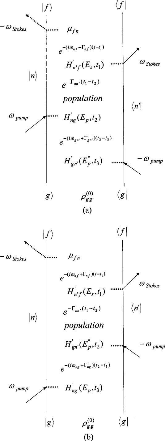
Feynman-type dual time-line diagrams for the third-order density matrix and polarization corresponding to hot luminescence, depicting the evolution of the bra vector on the right and the ket vector on the left, for each diagram, with interactions $H_{jk}^{\prime }$ between the system and the fields at times t ₃ ,t ₂ ,t ₁ and closure at time t. In (a) the pump interaction acts first on the bra 〈g| while in (b) it is the ket |g〉.

It is advantageous to be able to cast Eqs. (45) and (54) or their corresponding polarizations in terms of vibrational wave packet propagation on the upper potential energy surface rather than as a sum over intermediate states ${\sum }_n\cdots$, so as to facilitate numerical evaluation of the matrix elements. We need to assume that lifetime broadening dominates the linewidths and is independent of the vibrational states. In this two electronic state problem, we shall assume a lifetime ${\Gamma }_1^{-1}$ in the lower electronic state with vibrational Hamiltonian Ĥ₁ , and a lifetime ${\Gamma }_2^{-1}$ for the upper electronic state with vibrational Hamiltonian Ĥ₂, and an electronic transition moment μ₁₂ between them. Taking the Hamiltonians to have angular frequency units, for convenience, the respective third-order polarizations corresponding to Eqs. (45) and (54) in the quantum description of FSRS then take the simpler form:

$$\begin{array}{cc}\hfill {\left[P^{\left(3\right)}\left(t\right)\right]}_{\mathit{RRS}}=& {\left(\frac{1}{i\hslash }\right)}^3{\int }_{-\infty }^{t}d{t}_1{\int }_{-\infty }^{t_1}d{t}_2{\int }_{-\infty }^{t_2}d{t}_3\langle f\mid {\mu }_{12}{e}^{(-i{\widehat{H}}_2-{\Gamma }_2∕2)(t-t_1)}{\mu }_{21}{E}_p\left(t_1\right)e^{(-i{\widehat{H}}_1-{\Gamma }_1∕2)(t_1-t_0)}\mid g\rangle p_{\mathit{gg}}^{\left(0\right)}\left(t_0\right)\hfill \\ \hfill & \times \langle g\mid e^{(i{\widehat{H}}_1-{\Gamma }_1∕2)(t_3-t_0)}{\mu }_{12}{E}_p^{\ast }\left(t_3\right)e^{(i{\widehat{H}}_2-{\Gamma }_2∕2)(t_2-t_3)}{\mu }_{21}{E}_s\left(t_2\right)e^{(i{\widehat{H}}_1-{\Gamma }_1∕2)(t-t_2)}\mid f\rangle ,\hfill \end{array}$$ (55)

$$\begin{array}{cc}\hfill {\left[P^{\left(3\right)}\left(t\right)\right]}_{\mathit{HL}}=& {\left(\frac{1}{i\hslash }\right)}^3{\int }_{-\infty }^{t}d{t}_1{\int }_{-\infty }^{t_1}d{t}_2{\int }_{-\infty }^{t_2}d{t}_3\langle f\mid {\mu }_{12}{e}^{(-i{\widehat{H}}_2-{\Gamma }_2∕2)(t-t_2)}{\mu }_{21}{E}_p\left(t_2\right)e^{(-i{\widehat{H}}_1-{\Gamma }_1∕2)(t_2-t_0)}\mid g\rangle p_{\mathit{gg}}^{\left(0\right)}\left(t_0\right)\hfill \\ \hfill & \times \langle g\mid e^{(i{\widehat{H}}_1-{\Gamma }_1∕2)(t_3-t_0)}{\mu }_{12}{E}_p^{\ast }\left(t_3\right)e^{(i{\widehat{H}}_2-{\Gamma }_2∕2)(t_1-t_3)}{\mu }_{21}{E}_s\left(t_1\right)e^{(i{\widehat{H}}_1-{\Gamma }_1∕2)(t-t_1)}\mid f\rangle \hfill \\ \hfill & +{\left(\frac{1}{i\hslash }\right)}^3{\int }_{-\infty }^{t}d{t}_1{\int }_{-\infty }^{t_1}d{t}_2{\int }_{-\infty }^{t_2}d{t}_3\langle f\mid {\mu }_{12}{e}^{(-i{\widehat{H}}_2-{\Gamma }_2∕2)(t-t_3)}{\mu }_{21}{E}_p\left(t_3\right)e^{(-i{\widehat{H}}_1-{\Gamma }_1∕2)(t_3-t_0)}\mid g\rangle p_{\mathit{gg}}^{\left(0\right)}\left(t_0\right)\hfill \\ \hfill & \times \langle g\mid e^{(i{\widehat{H}}_1-{\Gamma }_1∕2)(t_2-t_0)}{\mu }_{12}{E}_p^{\ast }\left(t_2\right)e^{(i{\widehat{H}}_2-{\Gamma }_2∕2)(t_1-t_2)}{\mu }_{21}{E}_s\left(t_1\right)e^{(i{\widehat{H}}_1-{\Gamma }_1∕2)(t-t_1)}\mid f\rangle .\hfill \end{array}$$ (56)

It is straightforward to read these integrals using Feynman-type dual time-line diagrams similar to those shown in Figs. 3 and 4, respectively, with separate evolution of the bra 〈g| and ket |g〉. Each integrand has two matrix elements, and in each matrix element the pump or probe field interacting with the transition dipole moment causes a change in electronic state and a transfer of a vibrational wave packet from one potential energy surface to another. Each of the matrix elements can be evaluated by appropriate wave packet propagation of an initial vibrational state |g〉 (or 〈g|) on the lower or upper potential energy surfaces and finally taking the overlap with the final vibrational state |f〉 (or 〈f|) which describes the Raman transition from |g〉 to |f〉.²⁰ Take Eq. (55) as an example. The matrix element

$$\langle g\mid e^{(i{\widehat{H}}_1-{\Gamma }_1∕2)(t_3-t_0)}{\mu }_{12}{E}_p^{\ast }\left(t_3\right)e^{(i{\widehat{H}}_2-{\Gamma }_2∕2)(t_2-t_3)}\times {\mu }_{21}{E}_s\left(t_2\right)e^{(i{\widehat{H}}_1-{\Gamma }_1∕2)(t-t_2)}\mid f\rangle ,$$

which describes the path for the bra 〈g| is interpreted as (i) a propagation of a bra 〈g| on the lower state surface 1 for a time (t ₃ − t ₀) with the propagator $e^{(i{\widehat{H}}_1-{\Gamma }_1∕2)(t_3-t_0)}$; (ii) multiplication by the electronic transition dipole moment interacting with the pump field at time t ₃ given by ${\mu }_{12}{E}_p^{\ast }\left(t_3\right)$, which sends the wave packet in (i) to the upper state surface 2; (iii) propagation of the wave packet on surface 2 for a time (t ₂ − t ₃) with the propagator $e^{(i{\widehat{H}}_2-{\Gamma }_2∕2)(t_2-t_3)}$; (iv) multiplication by the electronic transition dipole moment interacting with the probe field at time t ₂ given by μ₂₁ E _s(t ₂), which sends the wave packet on surface 2 to the lower state surface 1; (v) propagation of the wave packet on surface 1 for a time (t − t ₂) with the propagator $e^{(i{\widehat{H}}_1-{\Gamma }_1∕2)(t-t_2)}$; and (vi) taking the overlap with the final vibrational state |f〉. The other matrix element $\langle f\mid {\mu }_{12}{e}^{(-i{\widehat{H}}_2-{\Gamma }_2∕2)(t-t_1)}{\mu }_{21}\times E_p\left(t_1\right)e^{(-i{\widehat{H}}_1-{\Gamma }_1∕2)(t_1-t_0)}\mid g\rangle$ has a similar interpretation, but this time using the ket |g〉.

In the quantum approach above, it was shown that the coupled-wave description of FSRS assumes a fundamental Raman transition from the ground vibrational state |g〉 = |0〉 to the first excited vibrational state |f〉 = |1〉. This is the most favored transition by virtue of the larger matrix element 〈1|Q|0〉, and in general for the matrix element 〈f|Q|g〉, the final vibrational state |f〉 = |g + 1〉 will be preferred for any initial state |g〉. In a time-resolved resonance Raman spectroscopy (TRRS), an ultrashort actinic pump pulse first prepares a nonstationary vibrational wave packet described by the density matrix ${\sum }_{g,g^{\prime }}{\rho }_{{\mathit{gg}}^{\prime }}^{\left(0\right)}\left(t_0\right)\mid g\rangle \langle g^{\prime }\mid$ on an excited electronic state which is subsequently probed, in the case here, by the new FSRS technique, as shown in Fig. 5, with the Raman pump and the Stokes probe frequencies being separated approximately by one vibrational quantum. To differentiate from the usual TRRS that uses a spontaneous Raman scattering probe, we may call this technique TRSRS (time-resolved stimulated Raman spectroscopy). The time resolution in this TRSRS experiment is given by the time difference between the intial wave packet preparation on the excited state surface by the ultrashort actinic pump pulse and the application of the ultrashort Stokes probe pulse in FSRS. This is independent of the frequency resolution of the FSRS gain profile which is governed by the duration of the Raman pump, the natural vibrational linewidth of the medium, and the resolution of the spectrograph. Equations (55) and (56) can readily be generalized to describe TRSRS where the ultrashort actinic pump pulse acts at time t ₀, as follows:

$$\begin{array}{cc}\hfill {\left[P^{\left(3\right)}\left(t\right)\right]}_{\mathit{RRS}}=& {\left(\frac{1}{i\hslash }\right)}^3\sum _{g,g^{\prime }}{\int }_{-\infty }^{t}d{t}_1{\int }_{-\infty }^{t_1}d{t}_2{\int }_{-\infty }^{t_2}d{t}_3\langle g+1\mid {\mu }_{12}{e}^{(-i{\widehat{H}}_2-{\Gamma }_2∕2)(t-t_1)}{\mu }_{21}{E}_p\left(t_1\right)e^{(-i{\widehat{H}}_1-{\Gamma }_1∕2)(t_1-t_0)}\mid g\rangle p_{{\mathit{gg}}^{\prime }}^{\left(0\right)}\left(t_0\right)\hfill \\ \hfill & \times \langle g^{\prime }\mid e^{(i{\widehat{H}}_1-{\Gamma }_1∕2)(t_3-t_0)}{\mu }_{12}{E}_p^{\ast }\left(t_3\right)e^{(i{\widehat{H}}_2-{\Gamma }_2∕2)(t_2-t_3)}{\mu }_{21}{E}_s\left(t_2\right)e^{(i{\widehat{H}}_1-{\Gamma }_1∕2)(t-t_2)}\mid g^{\prime }+1\rangle ,\hfill \end{array}$$ (57)

$$\begin{array}{cc}\hfill {\left[P^{\left(3\right)}\left(t\right)\right]}_{\mathit{HL}}=& {\left(\frac{1}{i\hslash }\right)}^3\sum _{g,g^{\prime }}{\int }_{-\infty }^{t}d{t}_1{\int }_{-\infty }^{t_1}d{t}_2{\int }_{-\infty }^{t_2}d{t}_3\langle g+1\mid {\mu }_{12}{e}^{(-i{\widehat{H}}_2-{\Gamma }_2∕2)(t-t_2)}{\mu }_{21}{E}_p\left(t_2\right)e^{(-i{\widehat{H}}_1-{\Gamma }_1∕2)(t_2-t_0)}\mid g\rangle p_{{\mathit{gg}}^{\prime }}^{\left(0\right)}\left(t_0\right)\hfill \\ \hfill & \times \langle g^{\prime }\mid e^{(i{\widehat{H}}_1-{\Gamma }_1∕2)(t_3-t_0)}{\mu }_{12}{E}_p^{\ast }\left(t_3\right)e^{(i{\widehat{H}}_2-{\Gamma }_2∕2)(t_1-t_3)}{\mu }_{21}{E}_s\left(t_1\right)e^{(i{\widehat{H}}_1-{\Gamma }_1∕2)(t-t_1)}\mid g^{\prime }+1\rangle \hfill \\ \hfill & +{\left(\frac{1}{i\hslash }\right)}^3\sum _{g,g^{\prime }}{\int }_{-\infty }^{t}d{t}_1{\int }_{-\infty }^{t_1}d{t}_2{\int }_{-\infty }^{t_2}d{t}_3\langle g+1\mid {\mu }_{12}{e}^{(-i{\widehat{H}}_2-{\Gamma }_2∕2)(t-t_3)}{\mu }_{21}{E}_p\left(t_3\right)e^{(-i{\widehat{H}}_1-{\Gamma }_1∕2)(t_3-t_0)}\mid g\rangle p_{{\mathit{gg}}^{\prime }}^{\left(0\right)}\left(t_0\right)\hfill \\ \hfill & \times \langle g^{\prime }\mid e^{(i{\widehat{H}}_1-{\Gamma }_1∕2)(t_2-t_0)}{\mu }_{12}{E}_p^{\ast }\left(t_2\right)e^{(i{\widehat{H}}_2-{\Gamma }_2∕2)(t_1-t_2)}{\mu }_{21}{E}_s\left(t_1\right)e^{(i{\widehat{H}}_1-{\Gamma }_1∕2)(t-t_1)}\mid g^{\prime }+1\rangle .\hfill \end{array}$$ (58)

The matrix elements for these integrals can be evaluated by a wave packet propagation procedure as described above. The implications of using various potentials and Raman pump and Stokes probe pulses on these results will be the subject of future work.

FIG. 5.

The femtosecond actinic pump pulse 1 prepares a vibrational wave packet on the excited electronic state which after a time delay is then subjected to FSRS using a narrow bandwidth Raman pump pulse 2 and a broadband Stokes probe pulse 3 which arrive simultaneously. The time resolution for the photochemical event is given by the time delay between the actinic pump and the Stokes probe pulses, while the frequency-resolution is given by the bandwidth of the Raman pump pulse, the vibrational dephasing time, the lifetime of the transient species, and the spectrograph resolution.

IV. CONCLUSION

We have presented both the coupled-wave and the quantum descriptions for femtosecond broadband stimulated Raman scattering, and have shown that the coupled-wave approach rests on several assumptions, of which the main ones are off-resonant Raman scattering and a fundamental Stokes Raman transition. When the Raman pump is on-resonance with an excited electronic state, the coupled-wave description is expected to break down, and the quantum approach should be used incorporating both the resonance Raman and the hot luminescence terms which allow for the population of vibrational levels on the excited electronic state reached by the Raman probe. The results for FSRS as a probe of a non-stationary vibrational wave packet prepared by an actinic pump pulse in a time-resolved stimulated Raman scattering experiment have also been presented.

References

- 1.Pelletier MJ. Appl. Spectrosc. 2003;57:20A. doi: 10.1366/000370203321165133. [DOI] [PubMed] [Google Scholar]
- 2.Myers AB, Mathies RA. Resonance Raman Spectra of Polyenes and Aromatics Vol. 12. In: Spiro TG, editor. Biological Applications of Raman Spectrometry. Wiley; New York: 1987. pp. 1–57. [Google Scholar]
- 3.Zhu L, Kim J, Mathies RA. J. Raman Spectrosc. 1999;30:777. [Google Scholar]
- 4.Louisell WH. Quantum Statistical Properties of Radiation. Wiley; New York: 1973. pp. 296–303. [Google Scholar]
- 5.Long DA. The Raman Effect: A Unified Treatment of the Theory of Raman Scattering by Molecules. Wiley; Chichester: 2002. [Google Scholar]
- 6.Levenson MD, Kano SS. Introduction to Nonlinear Laser Spectroscopy. Academic; San Diego: 1988. [Google Scholar]
- 7.Shen YR. The Principles of Nonlinear Optics. Wiley; New York: 1984. [Google Scholar]
- 8.Woodbury EJ, Ng WK. Proc. IRE. 1962;50:2367. [Google Scholar]
- 9.Eckhardt G, Hellwarth RW, McClung FJ, Schwarz SE, Weiner D, Woodbury EJ. Phys. Rev. Lett. 1962;9:455. [Google Scholar]
- 10.McCamant DW, Kukura P, Mathies RA. J. Phys. Chem. A. 2003;107:8208. doi: 10.1021/jp030147n. [DOI] [PMC free article] [PubMed] [Google Scholar]
- 11.McCamant DW, Kukura P, Mathies RA. Appl. Spectrosc. 2003;57:1317. doi: 10.1366/000370203322554455. [DOI] [PMC free article] [PubMed] [Google Scholar]
- 12.Kukura P, McCamant DW, Davis PH, Mathies RA. Chem. Phys. Lett. 2003;382:81. [Google Scholar]
- 13.Yoshizawa M, Kurosawa M. Phys. Rev. A. 1999;61:013808. [Google Scholar]
- 14.Placzek G. In: Handbuch der Radiologie. Marx E, editor. Vol. 6. Academische Verlagsgesellschaft; Leipzig: 1934. p. 205. [English translation by A. Werbin, UCRL Trans-526(L)] [Google Scholar]
- 15.Kramers HA, Heisenberg W. Z. Phys. 1925;31:681. [Google Scholar]; Dirac PAM. (A).Proc. R. Soc. London. 1927;114:710. [Google Scholar]
- 16.Bloembergen N, Shen YR. Phys. Rev. Lett. 1964;12:504. [Google Scholar]; Shen YR, Bloembergen N. Phys. Rev. A. 1965;137:1787. [Google Scholar]
- 17.Jackson JD. Classical Electrodynamics. 2nd McGraw-Hill; New York: 1975. pp. 13–17. [Google Scholar]
- 18.Lee SY, Zhang DH, Yoon SW, Mathies RA. (unpublished) [Google Scholar]
- 19.Shen YR. Phys. Rev. B. 1974;9:622. [Google Scholar]
- 20.Lee SY, Heller EJ. J. Chem. Phys. 1979;71:4777. [Google Scholar]; Pollard WT, Lee SY, Mathies RA. ibid. 1990;92:4012. [Google Scholar]