Abstract
Background
We propose a new method for supervised learning from gene expression data. We call it 'tree harvesting'. This technique starts with a hierarchical clustering of genes, then models the outcome variable as a sum of the average expression profiles of chosen clusters and their products. It can be applied to many different kinds of outcome measures such as censored survival times, or a response falling in two or more classes (for example, cancer classes). The method can discover genes that have strong effects on their own, and genes that interact with other genes.
Results
We illustrate the method on data from a lymphoma study, and on a dataset containing samples from eight different cancers. It identified some potentially interesting gene clusters. In simulation studies we found that the procedure may require a large number of experimental samples to successfully discover interactions.
Conclusions
Tree harvesting is a potentially useful tool for exploration of gene expression data and identification of interesting clusters of genes worthy of further investigation.
Background
In this paper we introduce 'tree harvesting' - a general method for supervised learning from gene expression data. The scenario is as follows. We have real-valued expression measurements for thousands of genes, measured over a set of samples. The number of samples is typically 50 or 100, but will be larger in the future. An outcome measurement is available for each sample, such as a survival time or cancer class. Our objective is to understand how the genes relate to the outcome.
The generic problem of predicting an outcome measure from a set of features is called 'supervised learning'. If the outcome is quantitative, the term 'regression' is used; for a categorical outcome, 'classification'. There are many techniques available for supervised learning: for example, linear regression, discriminant analysis, neural networks, support vector machines, and boosting. However, these are not likely to work 'off the shelf', as expression data present special challenges. The difficulty is that the number of inputs (genes) is large compared with the number of samples, and they tend to be highly correlated. Hastie et al. [1] describe one simple approach to this problem. Here we build a more ambitious model that includes gene interactions.
Our strategy is first to cluster the genes via hierarchical clustering, and then to consider the average expression profiles from all of the clusters in the resulting dendrogram as potential inputs into our prediction model. This has two advantages. First, hierarchical clustering has become a standard descriptive tool for expression data (see, for example, [2]), so by 'harvesting' its clusters, the components of our prediction model will be convenient for interpretation. Second, by using clusters as inputs, we bias the inputs towards correlated sets of genes. This reduces the rate of overfitting of the model. In fact we go further, and give preference to larger clusters, as detailed below.
The basic method is described in the next section for a quantitative output and squared error. We then generalize it to cover other settings such as survival data and qualitative responses. Tree harvesting is illustrated in two real examples and a simulation study is described to investigate the performance of the method. Finally, we generalize tree harvesting further, allowing nonlinear expression effects.
Results
Tree harvesting
As our starting point, we have gene expression data xij for genes i = 1,2, ...p and samples j = 1,2 ...n, and a response measure y = (y1, y2, ... yn) for each sample (each yj may be vector-valued). The response measure can take many forms: for example, a quantitative measure such as percentage response to a treatment, a censored survival time, or one of K cancer classes. The expression data xij may be from a cDNA microarray, in which case it represents the log red to green ratio of a target sample relative to a reference sample. Or xij might be the expression level from an oligonucleotide array.
The basic method has two components: a hierarchical clustering of the gene expression profiles, and a response model. The average expression profile for each cluster provides the potential features (inputs) for the response model.
We denote a cluster of genes by Xc, and the corresponding average expression profile by  c = (
c = ( c,1,
c,1,  c,2, ...
  c,n). Starting with p genes, a hierarchical clustering agglomerates genes in p - 1 subsequent steps, until all genes fall into one big cluster. Hence it generates a total of p + (p - 1) = 2p - 1 clusters, which we denote by c1, c2, ... c2p - 1.
The response model approximates the response measurement by some of the average gene expression profiles and their products, with the potential to capture additive and interaction effects. To facilitate construction of the interaction model, we translate each xij to have minimum value 0 over the samples:
![]()
The notation  denotes the average expression profile for a cluster c, using these translated values. The translation is done solely to make interactions in the model more interpretable. Note that the untranslated values are used in the clustering.
For a quantitative response yj, j = 1,2,...n, the model takes the form:

where βk and βkk' are parameters that are estimated by minimizing the sum of squared errors ∑j (yj -  j)2. As each
  has minimum value 0, the product terms represent positive or negative synergy between the genes involved.
Clearly it is not feasible, or even desirable, to include all clusters in the sums in Equation 2. Instead we build up the model in a forward stepwise manner as follows. Initially the only term in the model  is the constant function 1. The candidate terms
  consists of all of the 2p - 1 average expression profiles
  . At each stage we consider all products consisting of a term in
  and a term in
  , and add in the term that most improves the fit of the model in terms of a score statistic S. We continue until some maximum number of terms
  have been added to the model.
For example, at the first stage we enter the best average expression profile  ; this corresponds to the product of
  and the constant function 1. The resulting model has the form
  j =
j =  0 +
0 +  1
1 ,j, where
  0,
0,  1 are found by least squares. At the second stage, the possible additions to the model are
  2
2 ,j or
,j or  12
12 ,j
,j ,j for some cluster c2.
In general, this algorithm can produce terms involving the products of three or more average expression profiles. However, the user can put an explicit limit on the order of interaction, I, allowed in the model. For simplicity of interpretation, in the examples here we set I = 2, meaning that products are limited to pairwise products. This is achieved by only considering single terms (non-products) in  as candidates in the second step.
Models with pairwise interactions as in Equation 2 are often used in statistical applications. The interactions are usually included in an ad hoc basis, after the important additive terms have been included. An exception is the MARS (multivariate additive regression spline) procedure of Friedman [3]. This is a general adaptive learning method, which builds up an interaction model as products of piecewise linear functions of the inputs. The model is built up in the same way as in the tree-harvest procedure. MARS is a very popular methodology and inspired some of the ideas in this paper.
There are crucial computational details that make this algorithm run fast enough for practical applications. First, before the forward stepwise process is started, we need the average expression profiles for all of the 2p - 1 clusters. This is achieved in a natural recursive fashion using the tree structure available after a hierarchical clustering: the average expression profile in a node is the weighted average of the two average profiles of the daughter nodes, where the weights are the sizes of the daughter nodes. Other node specific statistics, such as variances and within-variances can be computed in a similar way.
Second, in the second step of the algorithm we must search over all 2p - 1 clusters to find the term that most improves the fit of the model. This is achieved by orthogonalizing the candidate average expression profiles with respect to the terms already in the model, and then computing a score test for each candidate term. With a quantitative response and least squares, this process gives exactly the contribution of each candidate term to the model. For survival, classification, and other likelihood-based models, it is a widely used approximation.
Additional features and issues
Data normalization
As with most sets of microarray experiments, the data for each experiment come from different chips and hence must first be normalized to account for chip variation. We assume that the values for each experiment j have been centered, that is xij →xij - (1/p) ∑ixij.
Choice of clustering method and criterion
The tree-harvest procedure just starts with a set of clusters, and these can be provided by any clustering method. We have chosen to base the procedure on hierarchical clustering, because of its popularity and effectiveness for microarray data (see, for example, [2]). The sets of clusters are conveniently arranged in a hierachical manner, and are nested within one another. Specifically if the clustering tree is cut off at two different levels, producing say four and five clusters, respectively, then the four clusters are nested within the five. Hence one can look at clusterings of all different resolutions at the same time. This feature is convenient for interpretation of the tree-harvest results, and is not a property of most other clustering methods. Despite this, other clustering methods might prove to have advantages for use in the tree-harvest procedure, including K-means clustering, self-organizing maps [4], and procedures that allow overlapping clusters (for example, gene shaving [1]). The choice of clustering criterion will also effect the results. Again, we have followed Eisen et al. [2] and used average linkage clustering, applied to the correlation matrix of the genes. The use of correlation makes the clustering invariant to scaling of the individual genes. Expanding the final clusters (see below) alleviates some of the sensitivity of the results to the choice of clustering method and criterion.
Biasing towards larger clusters
Typically gene expression datasets have many highly correlated genes. In addition, most clusters considered in the harvest procedure are subsets of other clusters. Hence if an average expression profile  is found to most improve the fit of the model in step 2 of the procedure, it is likely that the average expression profile of some larger cluster, perhaps containing the chosen cluster, does nearly as well as
  . Now all else being equal we prefer larger clusters, because they are more likely to be biologically meaningful. Large clusters can result from a pathway of genes involved in a biological process, or a heterogeneous experimental sample containing different cell types. In addition, the finding of a large cluster correlated with the outcome is less likely to be spurious than that of a small cluster, because there are many more smaller clusters than larger clusters. For these reasons, we bias the selection procedure towards larger clusters. Specifically, if the score for the cluster c is Sc, we chose the largest cluster c' whose score Sc' is within a factor (1 - α) of the best, that is satisfying Sc' ≥ (1 - α) Sc. The parameter α may be chosen by the user: we chose α = 0.10 in our examples. The cluster c' often contains some or all of the genes in c, but this is not a requirement. Although this biases the selection towards larger clusters, a single gene can still be chosen if its contribution is spectacular and unique.
Model size selection and cross-validation
Having built a harvest model with some large number of terms, M, we carry out a backward deletion, at each stage discarding the term that causes the smallest increase in sum of squares. We continue until the model contains only the constant term. This gives a sequence of models with numbers of terms 1,2, ... M, and we wish to select a model size, and hence one of these models. The model size is chosen by K-fold cross-validation. The data is split into K parts. For each k = 1,2, ... K the harvest procedure is trained on all of the data except the kth part, and then data in the kth part is predicted from the trained model. The results are averaged over k = 1,2, ... K. This is illustrated in the examples in the next two sections.
Expanding the clusters
Hierarchical clustering uses a sequence of discrete partitions of genes. Hence, for a given cluster, there may be genes not in that cluster that are more highly correlated with the cluster's average expression profile than some of the genes in the cluster. To account for this, we simply look for such genes in the final set of clusters and report them as 'extra genes' belonging to each cluster.
We summarize all of the steps in Algorithm 1 (Box 1)
Box 1.
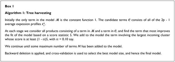
Algorithm 1: Tree harvesting.
Tree harvesting for general response variables
The tree-harvest method can be applied to most commonly occurring types of response data. Given responses y =(y1, y2, ... yn), we form a model-based approximation η =(η1, η2, ... ηn) to minimize a loss function:
![]()
Each quantity ηj is a function of the average gene expression profiles, having the form given in Equation 2:

Some common response types and loss functions are listed in Table 1.
Table 1.
Some common response types and loss functions
| Response type | Loss function |
| Quantitative | Sum of squares ∑j(yj-ηj)2 |
| Censored survival time | Partial log-likelihood |
| Categorical | Multinomial log-likelihood |
As outlined in the previous section, the model is built up in a forward stepwise manner. Considering  to be a function of the parameters β = {βk, βk,k'}, addition of each new term to the model is based on the size of the score statistic:

and similarly for βk,k'. The censored survival time and categorical response models are illustrated in the next two sections.
Survival of lymphoma patients
Figure 1 shows the dataset used in this example consisting of 3,624 gene expression measurements on 36 patients with diffuse large cell lymphoma (DLCL). These data are described in Alizadeh et al. [5]. The column labels refer to different patients, and the row labels identify the genes. We have applied hierarchical clustering to the genes and a separate clustering to the samples. Each clustering produces a (non-unique) ordering, one that ensures that the branches of the corresponding dendrogram do not cross. Figure 1 displays the original data, with rows and columns ordered accordingly.
Figure 1.
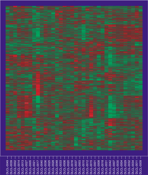
The DLCL expression matrix, with rows and columns ordered according to a hierarchical clustering applied separately to the rows and columns.
For each of the 36 patients, a (possibly censored) survival time is available; these range from 1.3 to 102.4 months, and 19 of the 36 patients died in the study period. An appropriate response model is Cox's proportional hazards model [6]. This has the form:
![]()
Here zj = (z1j, z2j, ... zmj) are m risk factors (features) for sample j, and h(t|zj) denotes the hazard function for an individual with feature values z; h0(t) is the baseline hazard function for an individual with risk factors z = 0. The unknown function r(zj) represents the log-relative risk of dying at any time t for an individual with z = zj versus an individual with z = 0. In the tree harvest model, the features (z1j, z2j, ... zmj) are average expression profiles and we take r(zj) to be of the form:
![]()
as in Equation 2. The tree-harvest algorithm computes an approximate score test from the partial likelihood, to decide which term is entered at each stage.
We ran the harvest procedure allowing a maximum of six terms, and it produced the results shown in Table 2.
Table 2.
Results of tree harvesting applied to lymphoma data
| Node | Parent | Score | -2log-likelihood | Size | |
| 1 | 3005 | 0 | 2.980 | 104.34 | 8 |
| 2 | 2236 | 3005 | 2.784 | 94.91 | 3 |
| 3 | 443 | 0 | 2.579 | 84.12 | 2 |
| 4 | s2461 | 3005 | 2.948 | 70.06 | 1 |
| 5 | s2188 | 3005 | 2.658 | 60.16 | 1 |
| Cox survival model fit to all five terms: | |||||
| Coef | exp(coef) | se(coef) | z | p | |
| z1 | 4.118 | 61.442 | 0.921 | 4.47 | 7.7e-06 |
| z2 | 1.072 | 2.922 | 0.293 | 3.66 | 2.5e-04 |
| z3 | 2.195 | 8.976 | 0.528 | 4.15 | 3.3e-05 |
| z4 | 1.079 | 2.941 | 0.281 | 3.83 | 1.3e-04 |
| z5 | -0.667 | 0.513 | 0.221 | -3.02 | 2.5e-03 |
Some explanation is needed. At each stage the 'Node' refers to the cluster whose average expression profile is chosen for addition to the model. 'Parent' is the number of the cluster, already in the model, that is to be multiplied by the Node average expression profile; Parent = 0 refers to the constant function 1. Nodes starting with 's' for Node or Parent indicate single genes. 'Score' is the score value achieved by addition of the term; it is roughly a Gaussian variate, so that values ≥ 2 are reasonably large.
Focusing just on the selection of the first cluster, Figure 2 shows all of the cluster scores. The green horizontal line is drawn at (1 - α) times the maximum score (α = 0.1), and we chose the largest cluster (blue point) above this line. This cluster is the eight-gene cluster 3005, shown in Figure 3.
Figure 2.
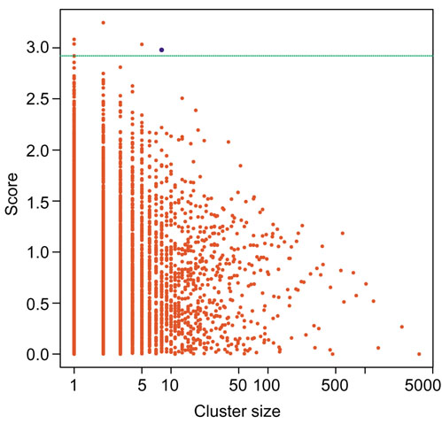
Scores for each cluster, from the first stage of the harvest procedure. The green horizontal line is drawn at (1 - α) times the maximum score, with α = 0.1. The largest cluster having a score above this line is chosen, indicated by the blue plotting symbol.
Figure 3.
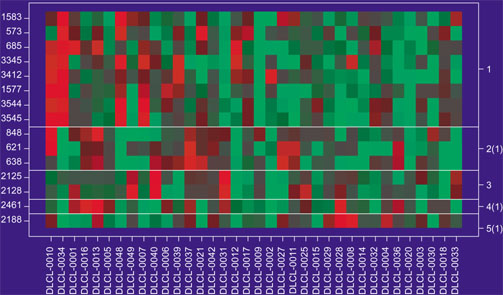
Lymphoma data. Clusters from tree harvest procedure, with columns in (expected) survival time order.
Overall the resulting model has the form:
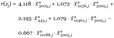
A positive coefficient indicates increased risk. The training set and cross-validation curves are shown in Figure 4. The minimum of the cross-validation (CV) curve occurs at one term, suggesting that the subsequent terms may not improve prediction.
Figure 4.
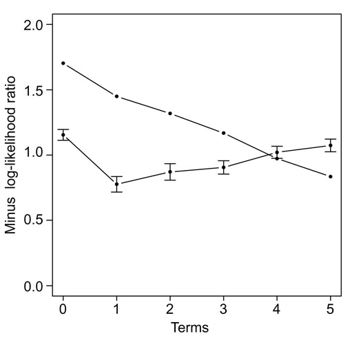
Lymphoma data. Training error curve (upper curve) and cross-validation error curve (lower curve with error bars).
The gene clusters are shown in Figure 3 and listed in the Additional data file, available with the online version of this article. Focusing only on the first cluster (3005), we computed the average expression for each of the 36 patients. Then the patients were divided into two groups: those with average expression below the median (group 1), and those with average expression above the median (group 2). The Kaplan-Meier survival curves for these two groups are shown in Figure 5 and are significantly different (p = 2.4 x 10⁻⁵).
Figure 5.
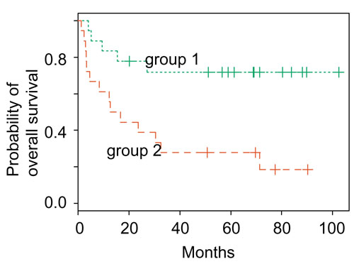
Survival curves of the two groups defined by the low or high expression of genes in the first cluster from tree harvesting. Group 1 has low gene expression, and group 2 has high gene expression. The survival in the groups is significantly different (p = 2.4 × 10⁻⁵).
If each of the 3,624 genes is ranked from lowest (1) to highest (3,624) value of the Cox score statistic, the average rank of the eight genes in the cluster 3005 is 3,574.5. Hence these genes are among the strongest individually for predicting survival, but are not the eight strongest genes. Rather they are a set of genes with very similar expression profiles, highly correlated with survival.
Human tumor data
In this example, the response is a categorical variable designating a cancer class. We use a subset of 61 of the tumors described in Ross et al. [7] and Scherf et al. [8], omitting the two prostate tumors and the one unknown class. There are expression values for 6,830 genes for each of the tumors, with the distribution across cancer classes shown in Table 3.
Table 3.
Distribution of gene expression across cancer class
| Breast | CNS | Colon | Leukemia | Melanoma | NSCLC | Ovarian | Renal |
| 9 | 5 | 7 | 8 | 8 | 9 | 6 | 9 |
NSCLC, non-small cell lung cancer
Here, the tree-harvest method builds a multiple logistic regression (MLR) model in a stepwise fashion, using similar steps to those used for the Cox model for survival data. The goal here is to model the probability of the tumor class, given the expression values. In general terms, if the class variable is denoted by y taking values in {1,2, ..., J} and the predictor variables by x1,x2, ..., xp a linear MLR model has the form:


As before, the x1 will be cluster averages, possibly individual genes, or pairwise products of these. The logistic transform is a natural scale on which to model the K probabilities; the inverse transformation:
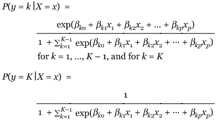
guarantees that the probabilities sum to 1 and are positive. The model is usually fit by multinomial maximum likelihood. Because the response is really multidimensional, we do not expect a single x to be able to distinguish all the cancer classes; this would imply that a single gene average creates an ordering that separates the cancer classes. Typically several are required.
At each stage, the tree-harvest algorithm considers augmenting the current fitted MLR model with a new term, candidates being any of the node averages, individual genes, or products of these with terms already in the model. As before, a score statistic is used, appropriate for the multinomial model.
The results of a tree harvest fit allowing seven terms are shown in Table 4. The deviance is a measure of lack-of-fit of the multinomial model, and we see that with seven terms in the model we have a saturated fit (the model produces probability estimates that are essentially 1 for each observation and the relevant class). This is almost certainly an overfit situation, since we are fitting 56 parameters to 61 observations.
Table 4.
Results of tree harvesting applied to human tumor data
| Node | Parent | Score | -2log-likelihood | Size | |
| 1 | 1177 | 0 | 6.48 | 197.53 | 6 |
| 2 | 3843 | 0 | 1.97 | 132.34 | 4 |
| 3 | 2008 | 0 | 1.78 | 79.34 | 3 |
| 4 | 1665 | 3843 | 0.85 | 71.01 | 3 |
| 5 | 5009 | 0 | 0.69 | 51.91 | 68 |
| 6 | 5087 | 2008 | 0.59 | 9.32 | 9 |
| 7 | 820 | 3843 | 0.55 | 0.00 | 2 |
Figure 6 shows all of the genes in the seven terms found by the model; the column order is chosen arbitrarily to separate the cancer classes (and is randomly chosen within cancer class). We used ten-fold cross-validation to find a good number of terms for the model. Figure 7 shows the results, in terms of the deviance statistic (-2 × log-likelihood). For these data, the two-term model minimizes the CV deviance curve and corresponds to the top two bands in Figure 6.
Figure 6.
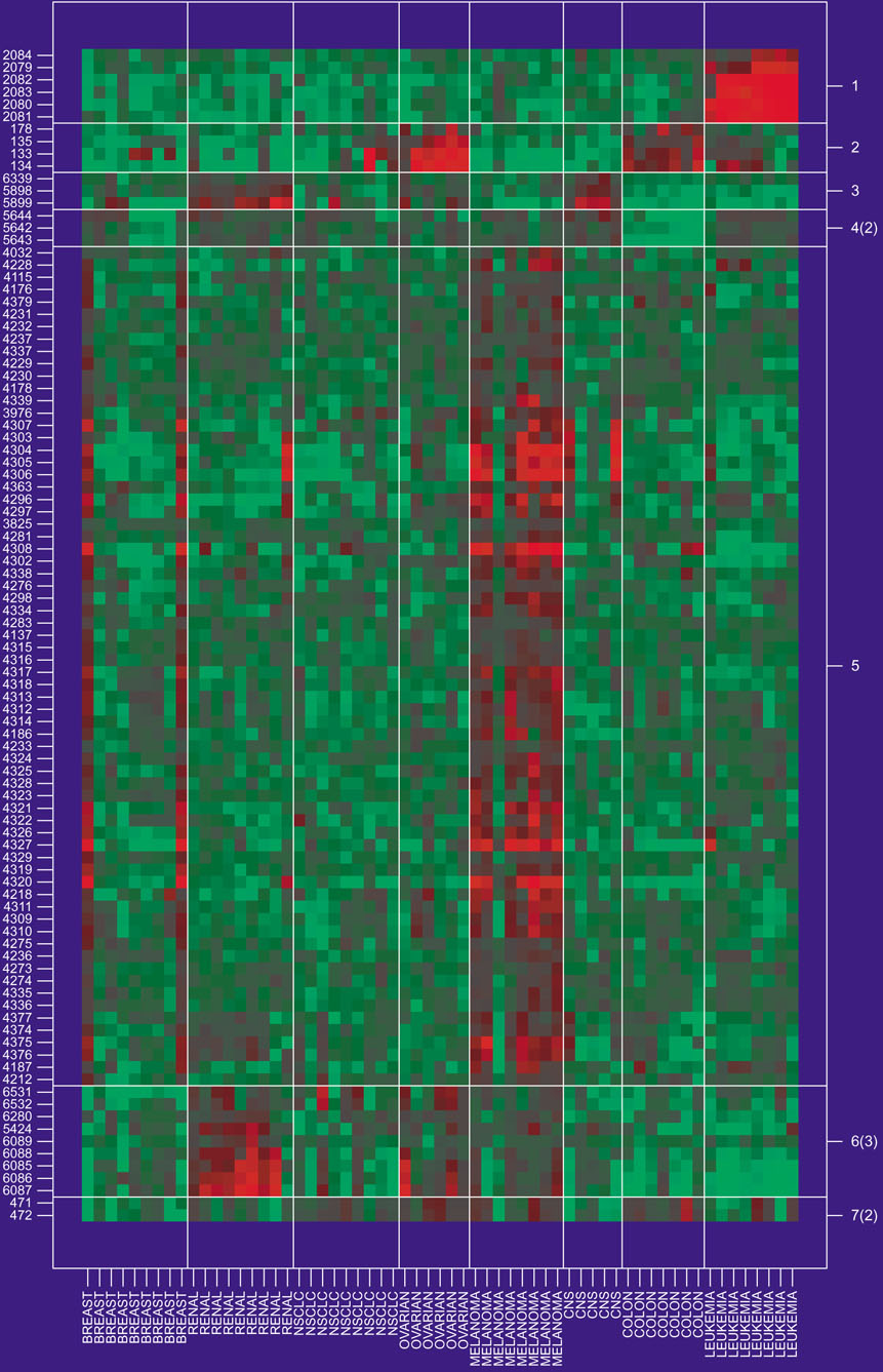
The seven clusters found by tree harvesting for predicting the tumor classes. They are ordered from top to bottom in terms of stepwise entry into the model. The vertical boundaries separate cancer classes.
Figure 7.
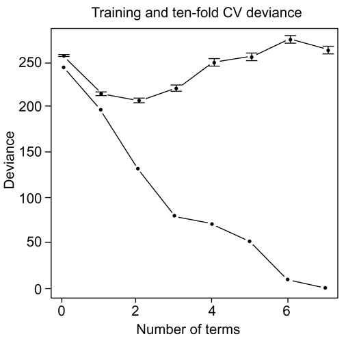
Model deviance for the tumor data. The lower curve is on the training data, and reaches 0 after seven terms (a saturated fit). The 0th term is the constant fit. The upper curve is based on ten-fold cross-validation, where care was taken to balance the class distribution in each fold.
Figure 8 shows a scatterplot of the average expression for each of the first two clusters, with samples identified by cancer class. Some clear separation in the cancer classes is apparent.
Figure 8.
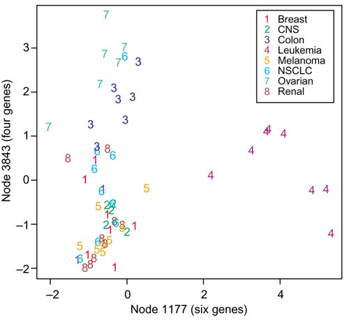
Plot of average expression for each of the first two clusters, with samples identified by cancer class. Some clear separation is apparent.
Simulations
We carried out a simulation experiment to assess how well tree harvesting discovers 'true' structure. To ensure that the gene expression measurements were realistic in magnitude and correlation, we used the matrix of 3624 × 36 lymphoma expression measurements for our study. Artificial survival and censoring times were then generated, to produce a simulated dataset for harvesting.
Two scenarios were considered, additive and interaction. For the additive scenario, we chose a cluster at random and generated the censored survival time with a relative risk of 2 as a function of its average expression profile. As indicated in Table 5, the randomly chosen cluster was taken from either single genes, small clusters (< 10 genes) or larger clusters (between 10 and 300 genes). Tree harvesting was allowed to enter just one term.
Table 5.
Simulation results
| Scenario | Average | Average | Proportion | Proportion | Average |
| number | number | of harvest | of true | correlation | |
| in | in | genes in | genes in | ||
| true | estimate | true | harvest | ||
| 3,624 total genes, 36 samples. Relative risk = 2.0 in additive scenarios | |||||
| p =1 | 1.0 | 2.4 | 0.80 | 0.80 | 0.86 |
| 2 <p < 10 | 3.4 | 4.8 | 0.60 | 0.60 | 0.91 |
| 10 <p <300 | 26.2 | 6.4 | 0.60 | 0.19 | 0.77 |
| Interaction | 3.4 | 2.6 | 0.28 | 0.21 | 0.65 |
| 3,624 total genes, 36 samples. Relative risk = 1.0 in additive scenarios | |||||
| p =1 | 1.0 | 1.6 | 0.24 | 0.60 | 0.61 |
| 2 <p <10 | 3.4 | 4.6 | 0.13 | 0.20 | 0.58 |
| 10 <p <300 | 26.2 | 3.8 | 0.40 | 0.21 | 0.61 |
| 1,622 total genes, 129 samples. Relative risk = 2.0 in additive scenarios | |||||
| p = 1 | 1.00 | 1.60 | 0.77 | 1.00 | 0.97 |
| 2 <p <10 | 2.80 | 3.00 | 0.93 | 1.00 | 0.99 |
| 10 <p <300 | 64.6 | 16.6 | 0.94 | 0.66 | 0.91 |
| Interaction | 9.4 | 7.6 | 0.85 | 0.87 | 0.86 |
The value p is the number of genes in the true underlying model.
For the interaction scenario, we randomly chose one cluster c1 with between two and ten genes, and then chose the second cluster c2 to be the cluster containing between two and ten genes whose average expression profile had the smallest correlation with that for c1. This made the two clusters as independent as possible, giving the harvest procedure the most chance of discovering their interaction. The survival data were then generated with relative risk function 4 + 4
+ 4 + 3[
+ 3[
 - r] where r is the projection of
 on
on  and
and  . Tree harvesting was allowed to enter three terms.
The results are shown in the top panel of Table 5. The numbers are averages over five simulations. The columns show the average number of genes in the true cluster, average number of genes in the cluster found by tree harvesting, the proportion of the genes found by tree harvesting that are in the true cluster, and vice versa. The final column shows the average absolute correlation of the average expression profile of the true cluster with the estimated cluster. For the interaction scenario, these quantities refer to the pooled set of genes that make up the interaction. If more than one interaction was found, the one having greatest overlap with the true interacting clusters is reported. We see that tree harvesting returns clusters that are a little too large when the true cluster is a single gene, and too small when the true cluster is large. In the additive scenario, it does a fairly good job at discovering the true cluster or one similar to it. However, it correctly discovers interactions only about a quarter of the time. A greater number of samples are needed to accurately find interactions among such a large set of genes. On the other hand, the correlations in the rightmost column are all quite high, indicating that tree harvesting is able to find clusters that are nearly as good as the true ones.
The middle panel of Table 5 shows the results for the additive scenarios when the relative risk is lowered to 1.0. As expected, they are somewhat worse, although the average correlations are still around 0.60.
To investigate whether a greater number of samples would improve the detection of interactions, we applied the same methodology to a set of 129 samples and 1,622 genes, from an unpublished study of breast cancer (T. Sorlie, C. Perou, and collaborators, personal communication). As before, we used the expression values and simulated sets of synthetic survival times. The results are shown in the bottom panel of Table 5. Now the tree-harvest procedure does a good job of recovering the interactions. The greater number of samples, together with the smaller number of genes, resulted in a significant improvement in performance.
Nonlinear tree-harvest models
In the harvest procedure described above, the effect of gene expression is modeled linearly. Thus, in modeling each term we assume that increasing or decreasing gene expression has a consistent effect on the outcome. However, it is biologically plausible for a gene to have a nonlinear effect: for example, increasing expression may correlate with longer survival, but only up to some level. Beyond that level, the same or worse survival might result.
To allow for nonlinear effects, flexible bases of functions could be used for each gene. However, with a large number of genes this would tend to overfit quickly. Hence we allow a simple quadratic function for each gene:
![]()
We first orthogonalize b(x) with respect to the linear term for the same gene, and then allow the transformed expression b(x) in place of the expression x in the tree-harvest model. In detail, the model has the same form as Equation 2:

where  equals either
  or
or  and γ is chosen to make
  uncorrelated with
  over the dataset.
If a quadratic term is multiplied by a positive coefficient, then the effect of a gene has a 'U' shape, decreasing and then increasing. For a negative coefficient, the effect is an inverted 'U'. A product interaction between two quadratic terms would indicate a strong synergistic effect between the two genes, with direction of expression (below or above average) ignored. When the nonlinear option is used in harvesting, the procedure tries both linear and nonlinear terms at each stage, and chooses the one with maximum score.
Lymphoma data continued
We tried tree harvesting with the nonlinear option for the lymphoma dataset, and it gave the first four terms shown in Table 6. Quadratic terms were entered in terms 2-4; these gave a better fit up to term 3 than the linear model fit earlier, but didn’t do as well after that. The clusters from this model are shown in Figure 9.
Table 6.
Results of nonlinear tree harvest procedure applied to lymphoma data
| Node | Parent | Score | -2Log-likelihood | Size | Nonlinear? | |
| 1 | 3005 | 2.980 | 104.34 | 8 | No | |
| 2 | s2597 | 0 | 3.891 | 91.18 | 1 | Yes |
| 3 | s1021 | 3005 | 3.919 | 81.59 | 1 | Yes |
| 4 | s583 | 3005 | 3.314 | 72.39 | 1 | Yes |
| Cox model fit to all 4 terms | ||||||
| coef | exp(coef) | se(coef) | z | p | ||
| z1 | 3.107 | 22.36 | 0.6551 | 4.74 | 2.1 × 10⁻⁶ | |
| z2 | 0.794 | 2.21 | 0.1990 | 3.99 | 6.6 × 10⁻⁵ | |
| z3 | 0.380 | 1.46 | 0.0954 | 3.98 | 6.8 × 10⁻⁵ | |
| z4 | 0.238 | 1.27 | 0.0729 | 3.27 | 1.1 × 10⁻³ | |
Figure 9.
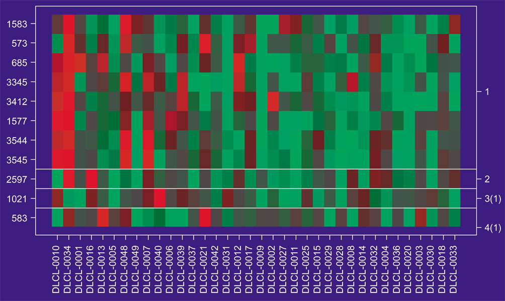
Lymphoma data: clusters from tree harvest nonlinear model, with columns in (expected) survival time order.
In the second cluster, for example (marked '2' in Figure 9), we see that survival time is greatest for moderate expression levels, and is worse for very low or very high levels.
Overall, the lack of significant improvement of the nonlinear model over the linear model gives greater confidence that the linear shape for each term is appropriate in this example. However, quadratic models may well be useful for other gene expression experiments.
Conclusions
The tree harvest procedure is a promising, general method for supervised learning from gene expression data. It aims to find additive and interaction structure among clusters of genes, in their relation to an outcome measure. This procedure, and probably any procedure with similar aims, requires a large number of samples to uncover successfully such structure. In the real data examples, the method was somewhat hampered by the paucity of available samples. We plan to try tree harvesting on larger gene expression datasets, as they become available. We used a forward stepwise strategy involving sum and products of the average gene expression of chosen clusters. We chose this strategy because it produces interpretable, biologically plausible models. Other models could be built from the average gene expression of clusters, including tree-based models or boosting methods (see, for example, Friedman et al. [9]).
Additional data
Additional data available with the online version of this article include clusters from the harvest model applied to lymphoma data.
Supplementary Material
Clusters from the harvest model applied to lymphoma data.
References
- Hastie T, Tibshirani R, Eisen M, Alizadeh A, Levy R, Staudt L, Botstein D, Brown P. 'Gene shaving' as a method of identifying distinct sets of genes with similar expression patterns. Genome Biology. 2000;1:research0003.1–0003.21. doi: 10.1186/gb-2000-1-2-research0003. [DOI] [PMC free article] [PubMed] [Google Scholar]
- Eisen M, Spellman P, Brown P, Botstein D. Cluster analysis and display of genome-wide expression patterns. Proc Natl Acad Sci USA. 1998;95:14863–14868. doi: 10.1073/pnas.95.25.14863. [DOI] [PMC free article] [PubMed] [Google Scholar]
- Friedman J. Multivariate adaptive regression splines. Annl Stat. 1991;19:1–141. [Google Scholar]
- Tamayo P, Slonim D, Mesirov J, Zhu Q, Kitareewan S, Dmitrovsky E, Lander E, Golub T. Interpreting patterns of gene expression with self-organizing maps: methods and application to hematopoietic differentiation. Proc Natl Acad Sci USA. 1999;96:2907–2912. doi: 10.1073/pnas.96.6.2907. [DOI] [PMC free article] [PubMed] [Google Scholar]
- Alizadeh A, Eisen M, Davis RE, Ma C, Lossos I, Rosenwal A, Boldrick J, Sabet H, Tran T, Yu X, et al. Distinct types of diffuse large B-cell lymphoma identified by gene expression profiling. Nature. 2000;403:503–511. doi: 10.1038/35000501. [DOI] [PubMed] [Google Scholar]
- Cox D. Regression models and life tables (with discussion). J Roy Stat Soc B. 1972;74:187–220. [Google Scholar]
- Ross D, Scherf U, Eisen M, Perou C, Spellman P, Iyer V, Rees C, Jeffery S, Van de Rijn M, Waltham M, et al. Systematic variation in gene expression patterns in human cancer cell lines. Nat Genet. 2000;24:227–235. doi: 10.1038/73432. [DOI] [PubMed] [Google Scholar]
- Scherf U, Ross DT, Waltham M, Smith LH, Lee JK, Kohn KW, Eisen MB, Reinhold WC, Myers TG, Andrews DT, et al. A gene expression database for the molecular pharmacology of cancer. Nat Genet. 2000;24:236–244. doi: 10.1038/73439. [DOI] [PubMed] [Google Scholar]
- Friedman J, Hastie T, Tibshirani R. Additive logistic regression: a statistical view of boosting. Annl Stat. 2000;28:337–374. [Google Scholar]
Associated Data
This section collects any data citations, data availability statements, or supplementary materials included in this article.
Supplementary Materials
Clusters from the harvest model applied to lymphoma data.


