Long Dynamics Simulations of Proteins Using Atomistic Force Fields and a Continuum Representation of Solvent Effects: Calculation of Structural and Dynamic Properties

Abstract

Long dynamics simulations were carried out on the B1 immunoglobulin-binding domain of streptococcal protein G (ProtG) and bovine pancreatic trypsin inhibitor (BPTI) using atomistic descriptions of the proteins and a continuum representation of solvent effects. To mimic frictional and random collision effects, Langevin dynamics (LD) were used. The main goal of the calculations was to explore the stability of tens-of-nanosecond trajectories as generated by this molecular mechanics approximation and to analyze in detail structural and dynamical properties. Conformational fluctuations, order parameters, cross correlation matrices, residue solvent accessibilities, pKa values of titratable groups, and hydrogen-bonding (HB) patterns were calculated from all of the trajectories and compared with available experimental data. The simulations comprised over 40 ns per trajectory for ProtG and over 30 ns per trajectory for BPTI. For comparison, explicit water molecular dynamics simulations (EW/MD) of 3 ns and 4 ns, respectively, were also carried out. Two continuum simulations were performed on each protein using the CHARMM program, one with the all-atom PAR22 representation of the protein force field (here referred to as PAR22/LD simulations) and the other with the modifications introduced by the recently developed CMAP potential (CMAP/LD simulations). The explicit solvent simulations were performed with PAR22 only. Solvent effects are described by a continuum model based on screened Coulomb potentials (SCP) reported earlier, i.e., the SCP-based implicit solvent model (SCP–ISM). For ProtG, both the PAR22/LD and the CMAP/LD 40-ns trajectories were stable, yielding C_α root mean square deviations (RMSD) of about 1.0 and 0.8 Å respectively along the entire simulation time, compared to 0.8 Å for the EW/MD simulation. For BPTI, only the CMAP/LD trajectory was stable for the entire 30-ns simulation, with a C_α RMSD of ≈ 1.4 Å, while the PAR22/LD trajectory became unstable early in the simulation, reaching a C_α RMSD of about 2.7 Å and remaining at this value until the end of the simulation; the C_α RMSD of the EW/MD simulation was about 1.5 Å. The source of the instabilities of the BPTI trajectories in the PAR22/LD simulations was explored by an analysis of the backbone torsion angles. To further validate the findings from this analysis of BPTI, a 35-ns SCP–ISM simulation of Ubiquitin (Ubq) was carried out. For this protein, the CMAP/LD simulation was stable for the entire simulation time (C_α RMSD of ≈1.0 Å), while the PAR22/LD trajectory showed a trend similar to that in BPTI, reaching a C_α RMSD of ≈1.5 Å at 7 ns. All the calculated properties were found to be in agreement with the corresponding experimental values, although local deviations were also observed. HB patterns were also well reproduced by all the continuum solvent simulations with the exception of solvent-exposed side chain–side chain (sc–sc) HB in ProtG, where several of the HB interactions observed in the crystal structure and in the EW/MD simulation were lost. The overall analysis reported in this work suggests that the combination of an atomistic representation of a protein with a CMAP/CHARMM force field and a continuum representation of solvent effects such as the SCP–ISM provides a good description of structural and dynamic properties obtained from long computer simulations. Although the SCP–ISM simulations (CMAP/LD) reported here were shown to be stable and the properties well reproduced, further refinement is needed to attain a level of accuracy suitable for more challenging biological applications, particularly the study of protein–protein interactions.

INTRODUCTION

Computer simulations have been extensively used to study the properties of liquids and solids.^1–5 They have also been useful for gaining insight into the structure, dynamics, and thermodynamics of individual molecules in the gas phase and in solution.⁶ In particular, molecular dynamics (MD) simulations can be carried out at a quantum mechanical (QM)^4,7 or molecular mechanical (MM)^6,8–10 level. For large molecular systems such as macromolecules, hybrid QM/MM approaches have been introduced.^11–13 The level of theory is dictated primarily by the problem to be studied and the size of the system, which in practice imposes limitations on the pure QM approach. Regardless of the type of calculation, application of these techniques to biological systems requires accounting for the effects of the solvent. The solvent modulates the structure of the solute, its dynamics and thermodynamic equilibrium. Because of the high computational demands, a complete atomistic description of solute and solvent is usually beyond the available resources. To reduce the computational problem, continuum approximations of solvent effects have been sought that allow removal of all or part of the solvent molecules but retain their effects on the solute of interest.^14–20 Although different degrees of physical rigor have been used to attain this goal, the effects of the solvent are usually introduced by a suitable modification of the Hamiltonian of the system. A physically meaningful continuum approximation would have an impact on all levels of theory, i.e., QM, QM/MM and MM calculations. The problem, however, is complicated because removing the solvent molecules eliminates or perturbs a number of effects that are difficult to describe quantitatively in a continuum description. Among the effects to be accounted for are bulk-solvent electrostatics, hydrophobicity and other solvent-induced intra-solute interactions (cooperative effects), energy modulation due to explicit hydrogen-bonding (HB) competition with solvent molecules, effects due to the granularity of the solvent, fluctuations in solvent density, electrostriction, pressure, and viscosity.⁸ Depending on the system of interest and the properties to be studied, one or more of these effects may need to be accurately described. A clear understanding of which of these effects may be dominant in a particular problem is essential for choosing the right approximation or model. For QM calculations of small molecules, a relatively small number of methods have been developed to introduce the effects of the solvent. In this case the emphasis has been placed mainly on the physical robustness of the approach.^16,21 On the other hand, the development of a physically realistic, yet practical continuum solvent model for macromolecules has been elusive, mainly because of the difficulties of representing all of the effects described above. Instead, an assortment of models and methods has been reported as MM approximations that range from purely statistical potentials to more physics-based approximations. Of necessity, simpler models have been traditionally used that provide a partial description of the solvent, which hopefully includes the dominant effects on the system. In biologically active macromolecules, solvent effects seem to be dominated mainly by electrostatics,^22,23 hydrophobicity,^24,25 and HB^26–28 interactions, all of which have been intensively studied in various contexts. Still, conceptual and practical difficulties remain in quantifying these effects, in particular the electrostatic^29–34 and hydrophobic^35–39 contributions. The description of HB has traditionally been ignored in continuum solvent approximations despite its fundamental role in controlling the structure and dynamics in macromolecules (cf. Materials and Methods). A minimal model of solvent effects for MM calculations of biological macromolecules should describe these three components of the energetics with a reasonable degree of realism.

Part of the difficulty encountered in developing a continuum model for biomolecules stems from their critical size scale. Proteins and nucleic acids, as well as other polymers, belong to the class of mesoscopic systems, where purely macroscopic concepts may not be justified on physical grounds and, at the same time, a purely atomistic description is not required. Both electrostatic and hydrophobic effects change regimes over size scales of typical biomolecules. Basic theoretical considerations show that the nature of the hydrophobic effect changes at length scales on the order of a nanometer.^35,36 On the other hand, basic electrostatic theory of polar/polarizable media and computer simulations of liquids show that the dielectric properties of water around a point charge/dipole change over distances of 5–10 Å,^15,34,40 and approach bulk properties only far from the solute. In biological systems, many interactions occur at the surface of molecules, or between molecules with characteristic length scales on the order of a nanometer or less. Therefore, a continuum solvent model for these mesoscopic systems should be formulated with consideration for this change in size regime. Nevertheless, simple implicit solvent models (ISM), including calculations in the gas phase (vacuum), have been used successfully in a variety of specific applications. However, experience has shown that it is usually not possible to know a priori whether such simplified models will work in a particular application. Thus, the main problems to resolve are the general reliability and transferability of a given approach. As the size and complexity of the systems grow, continuum models appear as the only viable alternative to a complete atomistic description, and reliability is requisite for success. Related to this is the problem of transferability of properties between different systems, which has been addressed and discussed for small molecules in a QM context,^41,42 and the possibility of using similar ideas in larger systems is appealing (SAH, unpublished). It is worth noting that a continuum approximation able to bridge the QM and the MM levels of theory may have the potential to evolve into a physically meaningful model for mesoscopic systems, including the possibility of minimizing the arbitrariness usually encountered in the development of parameters for ISMs in MM forcefields (see Discussion in ref. 16).

In an attempt to address some of the issues discussed above, a continuum approximation of electrostatic effects was proposed that is based on the theory of polar/polarizable liquids. This approximation describes the solvent molecules by Langevin dipoles that reorient and further polarize due to the field created by the solute, and are subject to thermal fluctuations, i.e., the approach proposed by Debye^15,34 (cf. Materials and Methods). The model is based on screened Coulomb potentials (SCP) and is currently being extended to provide a more accurate description of HB energetics.⁴³ The refinement of HB includes the effects due to the competition experienced by solvent-accessible residues for HB formation with the solvent and with other acceptors or donors in the protein (cf. Materials and Methods). In this article, the potential of this continuum approximation of solvent effects for structure and dynamics calculations of macromolecules is investigated. The reliability of the results obtained from such calculations is probed and the limitations discussed. The immediate goal of these calculations is to quantify structural and dynamical properties of proteins using long Langevin dynamics (LD) simulations and to compare the results with available experimental data and with results from explicit solvent simulations. This article is a continuation of a set of previously reported studies in which the basic computational approach was introduced and preliminary tests reported.^8,15,34

The article is organized as follows: Materials and Methods describes the methodology used and the computational setup; solvent electrostatic effects are discussed and the SCP continuum approach is briefly reviewed; the importance of a correct description of HB interactions in a continuum approach is discussed. In Results and Discussion, the results are presented and analyzed in detail; structural and dynamic properties are calculated, including pH-dependent effects and order parameters; a comparison with explicit solvent simulations and available experimental data is presented. The Discussion subheading provides a summary, and future directions are discussed.

MATERIALS AND METHODS

Electrostatic Effects

Consider a charge q immersed in an arbitrary dielectric medium. It is always possible to define a screening function D(r) such that the electric potential at position r can be expressed as φ(r) = q/D(r)r. The relationship between the physically measurable dielectric function ∊(r) and the screening function D(r) is found from the definition E(r) = −∇φ(r). For a single particle (spherical symmetry) in a pure solvent, the relation between both quantities is given by¹⁵

$$∊(r)=D(r){\left[1+\frac{r}{D(r)}\frac{d}{dr}D(r)\right]}^{-1}$$ (1)

While eq. (1) is exact, it has no information about the functional form of either ∊(r) or D(r), but the latter can be obtained from eq. (1) once the dielectric function ∊(r) is known from theoretical considerations or experiments. Experiments suggest that the dielectric function ∊(r) has a sigmoidal dependence with the distance,^44–50 which is supported by classical electrostatic theory of polar liquids (e.g. refs. ^15,51,52). The formal derivation of ∊(r) and its sigmoidal form was reported earlier⁵¹ and is based on the theory of polar solvation developed by Lorentz, Debye and Sack^51,53–57 (LDS theory; see review in ref. 58). It has been shown that Onsager’s reaction field effects⁵⁷ can also be incorporated into the formalism.^15,51 Eq. (1) shows that D(r) is also sigmoidal and approaches the same asymptotic value as ∊(r) as r increases. For a single point charge immersed in a pure solvent (e.g. water, acetone, or form-amide) composed of molecules with permanent dipole moment μ and polarizability p, the exact form of ∊(r) was derived earlier^51,52 and is given by

$$\begin{array}{l}∊(r)=1+\frac{{∊}_{\infty }-1}{{∊}_{\infty }+2}[∊(r)+2]\\ +\frac{4\pi \mu }{Qv}{r}^2∊(r)L\left\{\frac{Q\mu [∊(r)+2]}{[3k_{B}T+\mu R(r)]r^2∊(r)}\right\}\end{array}$$ (2)

where L(x) = coth(x) − 1/x is the Langevin function, R is the magnitude of Onsager reaction field, which can be expressed in terms of ∊(r),⁵¹ ∊_∞ is the high frequency permittivity (related to the polarizability through the Lorenz-Lorentz relationship, i.e., 4πp/3ν = [∊_∞ − 1)/(∊_∞ + 2)] Q is the charge of the source, μ is the magnitude of the dipole moments μ, ν is the solvent molecular volume, k_B is the Boltzmann constant and T is the temperature. From eq. (2) ∊(r) can be calculated at any point r, contains no adjustable parameters and is completely defined in terms of physically measurable quantities. For a numerical calculation of ∊(r) in pure solvents, see refs. ¹⁵ and ⁵¹. When a point dipole μ_s is the source of the field, an equation similar to eq.(2) is obtained for ∊(r) after proper Boltzmann averaging over all source orientations.⁵¹ Although not required from a theoretical standpoint, this second average over the source degrees of freedom allows recovery of the spherical symmetry that is otherwise broken by the fixed orientation of the source dipole. If the statistical average over the source is not performed, a sigmoidal screening is still obtained, but the exact form now is also dependent on the azimuthal angle defined by the vector position r and the orientation of the dipole source μ_s.⁵¹ It may already be noticed that a continuum formulation based on the LDS theory can be directly related to atomic properties of a molecule, i.e., local charges, Q, and to local dipoles, μ_s, which in turn may be obtained using approximate quantum chemical calculations.^{41,42,59–61} This procedure would formally link the screening functions D(r) of eq. (2) with the molecular electron density obtained from ab initio calculations.⁶²

Formulation of the Screened Coulomb Potential–Implicit Solvent Model (SCP–ISM)

An overview of the SCP continuum model of solvent effects (SCP–ISM hereafter) is given below (for details, see refs. ^8,15,34,63). Details of the implementation into the CHARMM force field (beta version c31b1) and other supplementary material are available in ref. 64. The SCP–ISM makes use of sigmoidal screening functions to characterize the damping of Coulomb interactions in a solvated protein. Thus, the model is based on D(r) not on ∊(r), and the precise form of D(r) is determined from the parameterization of the model. Sigmoidal screening functions were first used in the study of bifunctional organic acids and bases,^44–46 and later in protein electrostatics, where they were first used to account for pKa shifts in proteins.⁶⁵

Formally, once ∊(r) is known, e.g., through eq. (2), the inversion of eq. (1) can be achieved by numerical integration to obtain D(r). From a practical point of view, however, it is useful to invert it analytically. Note that a first-order differential equation with sigmoidal solutions would suffice. Such a differential equation was proposed previously⁶⁵ and has the form

$$dD(r)/dr=\lambda (1+D(r))(D_s-D(r))$$ (3)

where D_s has the value of the bulk dielectric constant and λ controls the rate of increase of D(r). Introducing this expression into eq. (1) yields a quadratic equation in D(r) and therefore an analytical expression of the screening as an explicit function of r and ∊(r). A solution of eq. (3) is given by D(r) = (1 + D_s)/[1 + k exp(−αr)] − 1, where k is a constant of integration that is set to (D_s − 1)/2 so that D(0) = 1, and α = λ (1 + D_s). By defining D(r) from a first-order differential equation with sigmoidal solutions, the physics of the system [i.e., Q, μ, μ_s, ∊_∞, p, etc; see eq. (2)] is implicitly contained in the parameters. Note that although any sigmoidal function could have been proposed as ∊(r) or D(r) (e.g., see discussion in ref. 16), the solutions of eq. (3) allow a good fit of the screening obtained from experimental data in pure solvents by adjusting the single parameter λ.⁶² Note that since λ (or α) depends in particular on atomic charges and dipoles of the solute, and it can be obtained from the LDS theory [cf. eqs. (1–3)], it is possible, in principle, to derive a first-order, parameter-free continuum model of solvation by combining quantum mechanics and theory of liquids.⁶² Since eqs. (1–3) are valid for a one-particle system, an atom-dependent modulating factor, δα should be added to α (yielding an effective screening α_eff = α + δα) to correct for the screening around each atom in an N-particle system, e.g., a polypeptide or nuclei acid. In the current version of the SCP–ISM, however, the atom-dependent parameters α_eff were obtained through the parameterization of the model based on solvation energies of single side-chain amino acid analogs,¹⁵ so the parameters obtained contain information of both α and the correction δα for such small molecules.

In the derivation of the SCP–ISM, the protein, composed of N partial charges q_i, reaches its final configuration in the solvent by following a standard thermodynamic cycle.^15,34 In this process, the work done in each step is evaluated, and the total electrostatic energy U_T of the macromolecule is calculated (non-electrostatic effects are treated separately). For calculating U_T, the potential is first expressed in the general form

$$\phi (r)=\sum _{i=1}^N\frac{q_i}{D(r)|r-r_j|}$$ (4)

for any arbitrary point r. The potential defined in eq. (4) is general and satisfies the Poisson equation regardless of the functional form of D(r) (as long as it is well behaved); it is assumed that D(r) and ∊(r) are scalar functions. The exact form of D(r) in eq. (4) is, of course, not known and is one of the fundamental questions in protein electrostatics. The simplifying approximation made for deriving the SCP–ISM is to assume that D(r) can be expressed in terms of distance-dependent screening functions D_s(|r − r_i|) of sigmoidal shape, centered at each atom coordinate r_i, and the potential is then expressed as a superposition of the form (index s stands for solvent, following notation in previously published work^15,34)

$$\phi (r)=\sum _{i=1}^N\frac{q_i}{D_s(|r-r_i|)|r-r_i|}$$ (5)

and then the position-dependent screening function D(r) is given in terms of the distance-dependent functions D_s(|r − r_i|) by D(r) = ∑_iq_i/|r − r_i|/∑_iq_i/|r − r_i|D_s(|r − r_i|). Note that D(r) is a continuous function of the position [except at (r_i)] and depends on the particular distribution of charges in the system, as expected. Note that these are formal expressions for the screening and potential that do not assume macroscopic concepts such as homogeneity of properties (constant dielectric) or sharp boundaries between solvent and solute.^8,34

When solvated, each particle polarizes the medium, creating a sigmoidal dielectric profile as described above. The energy U_i of the particle i in such a non-homogenous medium can be calculated using the basic expression⁶⁶

$$U_i=\frac{1}{8\pi }\int E_i(r)\cdot D_i(r)dv$$ (6)

where the integration is performed over the volume of the solvent (assumed to be infinitely extended); E_i(r) and D_i(r) are the electric and displacement fields of particle i in the medium. Using eq. (1), the integration in eq. (6) can be carried out analytically, with no approximations,^15,34 and yields the expression $U_i=q_i^2/2R_i{D}_s(R_i)$, where R_i is the lower limit of integration. Therefore, the work required to solvate each particle can be approximated by the Born equation of ion solvation⁶⁷ even in an inhomogeneous medium, but using the nonlinear, distance-dependent screening function D(r), i.e.,

$$\mathrm{\Delta }{U}_i=\frac{q_i^2}{2R_{i,B}}\left[\frac{1}{D_s(R_{i,B})}-1\right]$$ (7)

where R_i,B is the Born radius of the particle (if the inhomogeneity is neglected and the dielectric is approximated by a constant ∊_s, ΔU_i takes the usual form of the Born equation for an ion).

In a similar way, using eq. (1) it is possible to calculate the energy (work) required to form the system by bringing one particle at a time into the growing macromolecule. Using the approach described in refs. ¹⁵ and ³⁴, the total electrostatic energy of the system is given by

$$U_T=\frac{1}{2}\sum _{i\ne j}^N\frac{q_i{q}_j}{D_s(r_{ij})r_{ij}}+\frac{1}{2}\sum _{i=1}^N\frac{q_i^2}{R_{i,B}}\left[\frac{1}{D_s(R_{i,B})}-1\right]$$ (8)

where the first sum is the interaction term and the second, the self-energy contribution. Eq. (7) is exact under the assumptions described above (see refs. ^{15, 34}, and ⁶⁴), and D_s(r) is the screening function, which is assumed to account for all the screening mechanisms in the system; R_i,B is the effective Born radius of atom i in the solvated macromolecule. The polar component, ΔG^pol, of the solvation energy, ΔG, can be similarly derived, and a general expression was reported elsewhere.^15,34 Properties of the SCP model and of eq. (8) in particular have been discussed in previous publications^8,15,34,63 (see also ref. 64).

To calculate U_T from eq. (8), the effective Born radii, R_i,B must first be evaluated. An approach based on the degree of exposure of the atom to the solvent was introduced earlier,¹⁵ in which the effective Born radius for atom i is expressed as R_i,B = R_i,wξ_i + R_i,p (1 − ξ_i), where R_i,w and R_i,p are the Born radii in bulk solvent and protein, respectively; ξ_i is the degree of exposure of atom i to the solvent. The value ξ_i is calculated from the solvent accessible surface area (SASA) of each atom in the protein, i.e., ${\xi }_i=SAS{A}_i/4\pi R_i^2$ where R_i is the van der Waals radius of atom i increased by the probe radius. Although a numerical evaluation of ξ_i was found to be adequate in Monte Carlo applications of the model,^68–70 the computation of derivatives required in MD simulations is computationally slow. Therefore, an analytic expression is used to calculate ξ_i that is based on a contact model proposed earlier.⁸ In this case, ξ_i is given by ${\xi }_i=[A_i-B_i{\mathrm{\Sigma }}_{i\ne j}exp(-C_i{r}_{ij})]/4\pi R_i^2,$ where the constants A_i, B_i, and C_i are obtained by maximizing the correlation of R_i,B calculated from the numerical evaluation of ξ_i, and this analytical form, as discussed in ref. 8. In this approach, Born radii incorporate information of the local structure of the environment around the atom; thus R_i,B changes with the conformation of the protein; R_i,B also depends on the charge of the atom to account for the asymmetrical location of the dipole moment in water molecules and for saturation effects as described.¹⁵

Treatment of HB

Despite the enthalpic cost required to remove a polar group from a polar solvent, charged or polar side chains are often found in the interior of native proteins.^71–73 Invariably, these groups form internal hydrogen bonds with other buried groups, partially compensating for the unfavorable desolvation enthalpy.^73–75 Experiments seem to suggest that burying a polar group may contribute more to protein stabilization than burying a nonpolar group,^73,76–78 even when entropic effects are considered. Theoretical calculations, on the other hand, have yielded inconclusive results because of their dependence on the approximations used in the theoretical model (see e.g. refs. ^73,79,80). Clarifying this issue is essential for a reliable continuum model of solvation: a deficient description of the delicate balance between the unfavorable desolvation energy and favorable stabilization due to the formation of HB may lead to an incorrect estimation of many thermodynamic properties, such as protein–protein and protein–ligand interactions, protein folding/unfolding, structure prediction, estimation of transition rates and binding free energies.

From a computational perspective, special treatment of HB is necessary for the reliability of continuum models, as previously discussed.^43,63 The main reason for this is that the new term introduced into the force field that incorporates the continuum [eq. (8) in the SCP–ISM] is derived irrespective of any inter-solute HB considerations, since only statistical concepts of bulk solvent are used both in the formulation and parameterization. Because HB are a very specific kind of interaction, their resulting strength and geometry is carefully reexamined in the SCP–ISM after the term U_T is introduced in place of the original Coulomb energy function (~q_iq_j/r_ij), valid and optimized for gas-phase calculations. Because a correct description of HB patterns and dynamics is critical for reliable results, the problem of correctly representing HB energies in continuum approximations of macromolecules should be explicitly addressed. This is done in the SCP–ISM, in which the short-range donor–acceptor interactions are stabilized independently of the strength of the long-range electrostatics controlled by the macroscopic screening^43,63 D(r).

The definition of the effective Born radius of a polar hydrogen is given in the SCP–ISM by R_i,Bs = R_i,wξ_i + R_i,Aζ_i + R_i,p(1 − ξ_i − ζ_i), where ζ is the fraction of the proton surface buried in the acceptor solvation sphere and R_i,A is a parameter that can be thought of as the Born radius of the proton in a hypothetical bulk proton-acceptor solvent (see details in ref. 63). The method in its original form has been shown to give self-energies that correlate well with results from Poisson–Boltzmann calculations.¹⁵ It is noted that ζ is also evaluated using a contact model approximation, although earlier applications used an analytical expression.⁸ In the SCP–ISM, the strength of HB interactions in solution can be fine tuned by adjusting the R_i,A of the shared proton. Preliminary parameterization of HB energies was based on earlier results of point mutations of solvent-exposed residues in proteins.^63,81 However, to better account for (i) the electrostatic modulation due to the bulk solvent and (ii) the modulation due to the explicit competition with water molecules for available HB, a systematic study of the intermolecular potentials of mean force between all possible side chain–side chain (sc–sc) HB interactions in proteins has been carried out.⁴³ HB energies were calculated using constrained MD simulations in an explicit solvent model. For the simulations reported in this paper, sc–sc HB energies are only partially described by this more accurate parameterization, but a complete implementation will be needed to study protein–protein interactions (cf. Discussion); side chain– backbone (sc– b) and backbone– backbone (b– b) interactions are described according to the original algorithm and parameterization as reported in ref. 63.

Computational Setup for the Dynamics Simulations

To prepare the structures for the simulations, all the crystallographic water molecules were removed from the crystal structures [Protein Data Bank (PDB) access codes: 1pgb for ProtG, 1bpi for BPTI, and 1ubq for Ubiquitin (Ubq)]. In the explicit water molecular dynamics (EW/MD) simulations, the 3-ns trajectory of ProtG reported in ref. 8 was used for further analysis. For comparison, a similar protocol using the water drop model with constraining shell⁸² was used here for BPTI. Following a previously reported simulation setup,^8,82 a sphere of TIP3 water molecules with a radius of 32 Å was built around the protein. Solvent molecules that overlapped protein atoms were removed, leaving a total of ≈5800 water molecules. The minimal distance between protein atoms and the surface of the water sphere was ≈15 Å and the surrounding, constraining shell had a thickness of 4 Å.⁸ The MD simulations were performed using CHARMM⁸³ in the micro-canonical ensemble with the all-atom PAR22 force field.⁸⁴ The energy of the whole system was first minimized, then heated to 298K in 6 ps, and equilibrated for 100 ps. Subsequently, a 4-ns trajectory was generated using the SHAKE algorithm and a cutoff of 13 Å for the nonbonded interactions; the Verlet integration algorithm was used in all EW calculations. Ionization states of titratable residues corresponded to those at pH 7, assuming standard pKa values. See ref. 8 for additional details on the simulation protocol.

For the simulations with the SCP–ISM LD were used to mimic frictional drag and random collision of the solvent on the solute molecules. The stochastic differential equation governing the motion of atom i is $m_i{\ddot{r}}_i=F_i-{\zeta }_i{\dot{r}}_i+f_i(t),$ where $m_i{\ddot{r}}_i$ is the net force acting on atom i, with m_i the mass and ${\ddot{r}}_i$ the acceleration; F_i is the sum of all forces exerted on atom i by other atoms explicitly present in the system; −ζ_i ${\dot{r}}_i$ is the drag force with friction coefficient, ζ_i; ${\dot{r}}_i$ is the velocity; and f_i is the random force. In all LD calculations, the Leapfrog algorithm³ was used with a time step of 1 fs to integrate the equations of motion; temperature was kept constant at T = 298K. No constrains were applied to the proteins in the minimization or the heating and equilibration stages. An atom-based 13-Å cutoff with a shifting function starting at 12 Å was applied. For simplicity, a constant friction coefficient ζ_i = 50 ps⁻¹ was used for the heavy atoms in the proteins; this value is close to that given in ref. 85. It should be noted, however, that the correct choice of ζ_i, and the LD protocol itself, are an integral part of a complete ISM and, as such, should be given particular consideration in certain classes of problems^85,86 (see Discussion). For each protein, one LD simulation used the PAR22 parameter set (PAR22/LD), while the second simulation used the CMAP (CMAP/LD) force field introduced recently.^87,88 This new potential has been developed to correct for some of the observed weaknesses of the dihedral energy term in the PAR22 force field,⁸⁹ and its performance is currently being investigated. Further empirical improvements of this dihedral potential will probably be necessary in the future to better describe properties of proteins in crystal structures and in solution, in detriment of the accuracy at the ab initio level of description, as initially conceived. A detailed and unambiguous comparison between the PAR22 and CMAP potentials would require long MD simulations in explicit solvent, thus avoiding some of the simplifications and/or artifacts introduced by a continuum model in development. Results from multi-nanosecond dynamics of the proteins studied here will be reported elsewhere. For comparison of the PAR22 and CMAP representations, relevant to this article, see Results and Discussion.

For the calculation of fluctuations and average structures, the last 2 ns of the EW trajectories were used for ProtG and BPTI. Because much longer trajectories were generated for the SCP–ISM calculations, it was possible to analyze the convergence of dynamic properties. Figure 1 gives the average C_α root mean square (RMS) fluctuations for time intervals ranging from 1 to 12 ns measured from the end of the ProtG and BPTI trajectories. It is observed that the 1-ns interval is too short, but at 2 ns the fluctuations are already near convergence, although small changes are still seen at the 4 ns interval. By 6 ns, all trajectories appear to have converged, and this interval has been used to calculate the positional fluctuations and average structures. The average C_α RMS fluctuation of the ProtG EW trajectory changes from 0.66 Å for the 1-ns interval to 0.72 for the 2-ns interval. Therefore comparisons between the EW and ISM results should be interpreted with caution. All average structures were energy minimized for 200 steps using the ABNR algorithm with the SCP–ISM. Only average values are reported for the quantities studied; statistical errors did not modify the main conclusions and are not reported.

Fig. 1.

Dependence of the convergence of the averaged C_α- RMS fluctuations on window size: ProtG: (•) PAR22/LD and (▪) CMAP/LD; BPTI: (▾) PAR22/LD and (▴) CMAP/LD. The time windows are measured from the end of the trajectory.

RESULTS AND DISCUSSION

Energy Surface of the Alanine Dipeptide

In a recent study³⁴ of the alanine dipeptide immersed in a continuum solvent described by the SCP–ISM, it was shown that the energy surface in the (φ,ψ)-space calculated with this solvent model and the PAR22 force field were in agreement with the energy surface calculated from an explicit water simulation using the same force field.⁹⁰ To understand the effect of the SCP–ISM but in combination with the CMAP force field, the alanine dipeptide energy surface was calculated as described previously.³⁴ The results are shown in Figure 2: Figures 2(a and b) show the contour plots of the energy surfaces calculated with the SCP–ISM and the PAR22 and the CMAP dihedral potentials in CHARMM, respectively; Figures 2(c and d) display the corresponding plots calculated in the gas phase. Contours are plotted relative to the global minimum ( $C_7^{\text{eq}}$ see Table I) at 1.5 kcal/mol intervals. Comparison of the upper panel with the lower shows the profound effect of the solvent on the energy surface of the dipeptide. In particular, the transition states change markedly, as well as the positions and energies of the minima.

Fig. 2.

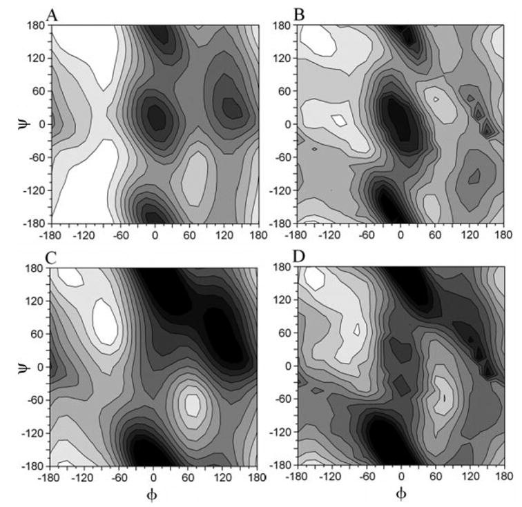
Contour plots of the energy surface of the alanine dipeptide calculated with the CHARMM force field (version c31b1): (a) SCP–ISM/PAR22, (b) SCP–ISM/CMAP, (c) VACUUM/PAR22, and (d) VACUUM/CMAP. The energy surfaces were calculated as reported in ref. 34, and contours are in increments of 1.5 kcal/mol.

TABLE I.

Relative Energies and Positions of Four Minima Found in Energy Surface of Alanine Dipeptide in Water as Represented by SCP–ISM/CHARMM Force Fields^a

	${\text{C}}_{\text{7}}^{\text{eq}}$	${\text{C}}_{\text{7}}^{\text{ax}}$	αR	αL
PAR22b	0.0 [−95,165]	3.5 [75,−85]	0.6 [−90,−75]	7.7 [60,40]
CMAP	0.0 [−162,164]	3.8 [56,−154]	1.2 [−104,0]	2.8 [63,45]

^aCalculations were carried out with version c31b1; all energies are in kcal/mol; angles (in square brackets) in degrees. Energies and angles were obtained with the software Origin; because of the grid spacing in the (φ,ψ)-plane, these values should be considered approximate.

^bThe small differences observed with respect to values reported in ref. 34 are mainly due to the pairwise energy function of the current version of the SCP–ISM introduced in ref. 8 which was used here both in the minimization and in the calculation of energies (minimization in vacuum was used in ref. 34, and a non-pairwise energy function was used in the energy calculations).

Comparison of the SCP–ISM/CMAP/CHARMM surface of Figure 2(b) with Figure 6 in ref. 91 and with Figures 1 and 2 in ref. 88 shows that the positions and energies of the minima are in qualitative agreement with previous QM/MM calculations as well as with statistical distributions obtained from a search in the PDB. This is in contrast to the SCP–ISM/PAR22/CHARMM surface shown in Figure 2(a), which tends to be populated almost exclusively in the −180° < φ < 0° region of the Ramachandran plot (compare with Fig. 3 in ref. 91). With the coarse-grained (φ,ψ)-grid used in these calculations, four minima were identified in the SCP–ISM surfaces [cf. Fig. 2(a and b)], corresponding to the ${\text{C}}_{\text{7}}^{\text{eq}},{\text{C}}_{\text{7}}^{\text{ax}},$α_R, and α_L minima and discussed previously (see Table I). The change in energy of the α_L minimum from about 7.6 kcal/mol with the SCP–ISM/PAR22 to about 2.8 kcal/mol with the SCP–ISM/CMAP is noteworthy. This shift in the energy minimum is important because it may dramatically affect structure calculations (e.g., using MC sampling). In particular the first residue in a type I′ β-hairpin should have values of its (φ,ψ) torsional angles in the α_L region.^92,93 This shift in energy may also affect the dynamics of proteins (see below). A similar degree of accuracy is expected from a quantitative comparison between the SCP–ISM/CMAP and similar EW/CMAP calculations of the alanine dipeptide energy surfaces.

Fig. 6.

C_α RMSF of (a) ProtG and (b) BPTI (symbols as in Fig. 5 observed in the PAR22/LD simulaton of). The fluctuations were calculated from the last 2 ns of the EW/MD simulations and the last 6 ns of the ISM/LD simulations. The fluctuations for the crystal structure were obtained from the B-factors (see text).

Fig. 3.

Temporal evolution of the C_α RMSD of (a) ProtG, (b) BPTI, and (c) Ubq. Black line: PAR22/LD; gray line: CMAP/LD. Insets: (a) EW/MD trajectory; (b) EW/MD (gray), PAR22/LD (black).

Trajectories

Three simulations were performed on the 56-residue protein ProtG and three on the 58-residue protein BPTI: for ProtG a 3-ns and for BPTI a 4-ns simulation in explicit water, along with two implicit solvent simulations of 40 ns for ProtG and 30 ns for BPTI. The three-dimensional structure of ProtG has been determined by X-ray crystallography⁹⁴ and NMR spectroscopy;⁹⁵ the two structures differ primarily in the loop involving residues 46–51, and other structural variations are observed in the helix.⁹⁴ ProtG contains a packed core of nonpolar residues located between a four-stranded β-sheet and a four-turn α-helix.⁹⁴ BPTI adopts a tertiary fold comprising two strands of antiparallel β-sheet and two short segments of α-helix.⁹⁶ Due to the long loops in the structure, BPTI is more flexible than ProtG. The structure of BPTI is stabilized by three disulfide bridges that can be observed in the stable folds that link cysteines 5 and 55, 14 and 38, and 30 and 51. A core of nonpolar residues is also present in this protein.

The time evolution of ProtG and BPTI are given in Figure 3(a and b). For each protein, the trajectories obtained from the PAR22/LD and the CMAP/LD simulations are presented, as welll as the corresponding EW/MD trajectories shown in the inset of each figure. The structure of ProtG remains stable in all trajectories as shown in Figure 3(a). Both LD trajectories closely follow the EW/MD trajectory (for the first 3 ns) and become stable after about 0.6 ns, while the EW/MD simulation becomes stable after about 1.5 ns. From Figure 3(a) it is observed that the two ISM/LD trajectories are practically identical for the entire 40 ns of the simulation.

Unlike ProtG, the PAR22 and CMAP force fields lead to quite different SCP–ISM trajectories for BPTI, as shown in Figure 3(b). The CMAP trajectory stabilizes after about0.5 ns of simulation and then remains stable for the entire 32 ns with an average C_α RMSD of about 1.4 Å. In contrast, the RMSD of the PAR22/LD trajectory starts to increase after about 3 ns [see Fig. 3(b)], first reaching a plateau at around 8 ns with an average RMSD of about 2.0 Å and then around 17 ns distorting still further from the crystal structure and reaching an average C_α RMSD of about 2.8 Å toward the end of the simulation. Note that the PAR22/LD trajectory remains stable for the first 3 ns of the simulation [see inset, Fig. 3(b)], showing that short simulation times may lead to incorrect conclusions regarding the stability of a particular simulation. The EW/MD simulation stabilizes after about 2 ns and then remains stable to the end of the 4-ns trajectory. Thus, for both proteins the SCP–ISM stabilizes the dynamics more rapidly than when solvent is represented explicitly, as has been observed previously.⁸

Backbone superpositions of the average structures of ProtG and BPTI on their crystal structures are shown in Figure 4. For ProtG, inspection of the superimposed structures shows that the average structures calculated from the simulations preserve the essential features of the experimental structure, including secondary and tertiary structural motifs and residue packing. On the other hand, in the case of BPTI only the CMAP/LD average structures superimpose well on the crystal structure, while the PAR22/LD structure shows significant deviations. The main sources of the distortion are the two long disulfide-bridged loops, with loop1 (residues 7–17) having an RMSD from the crystal structure of 2.3 Å and loop2 (residues 36 – 47) having an RMSD of 1.7 Å. The RMSD of the other elements of the secondary structure have relatively small deviations from the crystal, with a C_α RMSD of less than 0.51 Å.

Fig. 4.

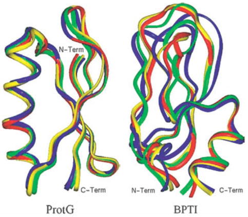
Ribbon representation of the superimposed average structures on the crystal structures for ProtG (left) and BPTI (right): red (crystal): green (EW/MD); blue (PAR22/LD); and yellow (CMAP/LD). EW/MD average structures were obtained from the last 2 ns of the trajectories, whereas the PAR22/LD and CMAP/LD average structures were obtained from last 6 ns of the trajectories.

The observations described above are presented quantitatively in Table II, in which various RMSD values between the average and crystal structures are given. The all-heavy atom and C_α RMSD of both molecules reflect the tendencies already seen in their structures and dynamics displayed in Figures 3 and 4. From Table II it is observed that the EW/MD and both ISM/LD simulations of ProtG yield similar RMSD values; in particular both the side chains and the backbone of the average structures are close to the crystal structure in all cases. However, for BPTI only the average structures calculated from the EW/MD and CMAP/LD simulations remain close to the experimental structure, while the RMSD of the PAR22/LD simulation becomes too large. In the last two rows of Table II, the residues have been divided into two classes based on whether the degree of burial of the side chains is greater or less than 0.7, and the all-heavy atom RMSD values of the side chains were calculated for each class. This threshold was chosen because it has been shown elsewhere^97,98 that the modulation of pH-dependent properties of side chains that are more than 30% solvent exposed is primarily controlled by the solvent, whereas for side chains that are more than 70% buried the protein environment controls the modulation. The results show that for both EW/MD and ISM/LD simulations, the deviations from the crystal structure conformations are smaller for buried residues than those that are solvent exposed. This finding is not unexpected given the much greater confinement of the buried residues, but it is important that this property is conserved by an ISM in long dynamics, as reported here. Note that this difference still holds for the PAR22/LD simulation of BPTI, but the all-heavy atom RMSD of the buried residues is >2 Å.

TABLE II.

Comparison of Average RMSD Values Obtained From Simulations of ProtG and BPTI

	ProtG			BPT1
Atom type	EW/MD	PAR22/LD	CMAP/LD	EW/MD	PAR22/LD	CMAP/LD
Alla	1.65	2.16	1.97	2.24	3.30	2.11
Cαb	0.81	0.99	0.84	1.54	2.73	1.42
Exp% > 0.3c	2.33	2.51	2.56	3.02	4.22	2.80
Exp% < 0.3d	1.57	1.75	1.58	1.62	2.44	1.59

^aRMSD (in Å) of all heavy atoms.

^bRMSD (in Å) of all C_α atoms.

^cRMSD (in Å) of all heavy atoms of side chains with average fractional solvent exposure >0.3.

^dRMSD (in Å) of all heavy atoms of side chains with average fractional solvent exposure <0.3.

To gain further insight into the origin of the structural distortion of BPTI in the PAR22/LD simulation, the (φ,ψ) angles have been plotted in Figure 5a for the EW/MD and both ISM/LD trajectories as well as the crystal structure. For the ISM/LD and EW/MD simulated structures, the values were taken from the average structure calculated from the last 6 and 2 ns, respectively. Inspection of the figure shows that the (φ,ψ) values of the CMAP/LD average structure are close to the values obtained from the crystal structure for all residues (neglecting the C-terminus residues 57 and 58). This is not surprising because the structure remains close to the crystal for the entire simulation time. In contrast, the (φ,ψ) values of the PAR22/LD average structure differ from the crystal structure values for several residues: T11, G12, C14, A16, R17, G36, G37, C38, and R39.

Fig. 5.

Residue-based (φ,ψ) torsion angles in the crystal and the average structures of (a) BPTI and (b) Ubq: ( ) EW/MD (red); ( ) PAR22/LD; (▾) CMAP/LD; and (▪) crystal structure. Approximate positions of the secondary structure elements are displayed schematically at the bottom of each figure: diagonal hatching: α-helix; open: β-strand; black: loop.

As discussed above, the two right hand quadrants of the Ramachandran plot are poorly represented by the PAR22 force field when compared to results from ab initio calculations.⁹¹ In particular, the α_L minimum is too high in energy relative to the absolute minimum and is not populated at room temperature. Similarly, the PAR22 potential surface of the glycine dipeptide is quite different from the ab initio surface, as shown by a comparison of Figures 10 and 12 in ref. 91. The PAR22 distribution of glycine also suggests that the energy of the α_L region is too high. This problem with the all-atom PAR22 force field is well known^34,91 (see above) and may contribute to structural instabilities of β-turn regions in proteins and peptides when long dynamics simulations or structural searches in Monte Carlo simulations are performed (SAH unpublished). Note that similar problems have been identified in other force fields (see ref. 91).

From Figure 5(a), it can be seen that all residues from the PAR22/LD simulation with deviant (φ,ψ) values (i.e., they differ by more than 60° from the crystal structure values) are in the loop segments of BPTI. The (φ,ψ) values of the crystal structure of residue R39 are (60°,70°), which puts this residue in the α_L region. Since PAR22 cannot access this region at the simulation temperature, these values of (φ,ψ) shift early in the dynamics to the upper-left quadrant (β-region) of the Ramachandran plot, reaching values around (−90°,150°) in the final average structure. Note that in BPTI there are no other residues with (φ,ψ) values in the α_L region, and in ProtG, there are no such residues.

Of the nine deviant residues (listed above), only for R39 are the experimental (φ,ψ) values in a region inaccessible to PAR22. For the four residues, C14, C38, A16, and R17 the (φ,ψ) values of the crystal structure are in the β-region, while in the ISM/LD simulation using PAR22, these residues are in the lower-left quadrant (α-region), and for T11 the crystal structure is in the α-region and the PAR22 average structure in the β-region. The three glycine residues behave similarly, putting the PAR22 structure in a different quadrant from the experimental structure. Because of the failure of PAR22 to properly describe the α_L region, the conformation of R39 in the PAR22/LD average structure (Fig. 5a) is strongly distorted. Assuming that the energy function correctly ranks the crystal structure as a member of the native ensemble at the absolute free energy minimum, it may be that the deviations found in the other eight residues in the PAR22/LD simulation are a collective response to the distorted R39 to maintain as far as possible the optimal, native structure.

Although the EW/MD simulation is much shorter than the ISM/LD simulations, it is instructive to examine the main chain torsion angles of the EW/MD average structure [see Fig. 5(a)] because the simulation also uses the PAR22 force field. It is seen that nearly all residues are in close agreement with the crystal structure except for R39 and G36. The (φ,ψ) values of R39 from the EW/MD average structure places it in the β-region, as is the case for the PAR22/LD conformation of R39. Figure 5a shows that the torsion angles of G36 in the PAR22/LD simulation also deviate strongly from the crystal structure values, making it tempting to suggest that the distortion in G36 compensates for the artifactual conformation of R39 to maintain the structure as near to the crystal structure as possible. It is noted that there are four other residues that show smaller differences (<60°) that may also compensate for the distortion introduced by R39.

To further probe the generality of the above findings, the analysis of the backbone torsional angles has been applied to long PAR22/LD (7 ns) and CMAP/LD (35 ns) simulations of Ubq. Ubq is a 76-residue protein comprising a three-turn α-helix and a five-strand β-sheet, packed together by a dense hydrophobic core. The last four residues (LRGG) on the C-terminus are solvent exposed both in the crystal⁹⁹ and in the NMR structures (PDB: 1d3z),¹⁰⁰ showing large conformational fluctuations and no HB interactions with the rest of the protein. The time evolution of the trajectory is given in Figure 3(c). Both dynamics show large conformational fluctuations of the last four residues, so they were excluded from the RMSD calculations. The CMAP trajectory is stable for the entire simulation time, with an average C_α RMSD of about 1 Å. The C_α RMSD of the PAR22 trajectory appears to be increasing, with a value of about 1.5 Å at 7 ns. However, the structure clearly has not distorted to unacceptable levels at this stage of the simulation, and a plateau is attained until at least 10 ns, when the simulation was interrupted. For the analysis below, an average structure from the last 2 ns of the PAR22 trajectory and the last 6 ns of the CMAP trajectory was used.

The φ and, ψ torsional angles for each residue are plotted in Figure 5(b). From the crystal structure of Ubq, there are six residues (T9, E34, F45, A46, Y59, and K63) with (φ,ψ) torsion angles in the range (48 – 81,5– 45). Figure 2(b) gives a range of (45–100,5–70) for the α_L region so that all six residues appear to fall in this region. Note that the standard range of (φ,ψ) values assigned to the α_L region is somewhat narrower.⁹² From Figure 5(b) it is seen that all six residues are located in the loop regions of the protein, as is the case for BPTI [Fig. 5(a)]. Figure 5(b) shows that the values of all torsion angles in the CMAP simulation are close to the corresponding crystal structure values, which is not the case for the PAR22 simulation. Of the six residues in the α_L conformation, three have distorted to other regions in the Ramachandran plot, namely F45 (65,− 85; 1 ns), A46 (−140,10; 1 ns) and K63 (−60,135; 4 ns), where the last entry is the time at which the residue is no longer in the α_L region. None of these residues have necessarily found their equilibrium conformations at this time in the simulation, which may also be true for the other three residues that are still in the α_L-region conformation at 7 ns. From these findings, it appears that the behavior observed in the PAR22/LD simulation of Ubq is similar to that found in BPTI. Thus there is a strong tendency for residues in the α_L region to find other more favorable conformations (for the PAR22 force field), and there are other residues, usually in the loops, that also distort [see Fig. 5(a and b)], perhaps as compensation to allow the protein to stay as close as possible to the actual solution structure. The fact that these residues are found in the loop segments, combined with their flexibility, allows them to adjust to conserve the overall solution conformation. Nevertheless, such distortions may lead to side-chain conformations very different from their actual conformations, which, in turn, may lead to large errors in the calculated values of other properties.

Fluctuations and Correlation of Motions

The RMS fluctuations (RMSF) of the C_α were calculated from the simulations and the Debye–Waller factors of the crystal structures¹⁰¹ and are shown in Figure 6. The approximate positions of the elements of secondary structure are also shown at the bottom of each panel. The RMSD between the calculated and experimental RMSF values were also calculated and are reported in the second column of Table III. Figure 6 shows that the RMSF calculated from the simulations exhibit a rough qualitative correspondence to the crystallographic B-factors in both proteins. However, larger deviations are apparent that, on average, are greater in BPTI than in ProtG (cf. Table III). It is noted, however, that this difference may be due to the much smaller window that was available for calculating the RMSF of the EW trajectories (see Fig. 1). Note also that for ProtG the RMSF-RMSD from the two ISM/LD simulations are very similar, while for BPTI the RMSD is larger for the PAR22/LD simulations, which might be another indicator of the large structural distortion of BPTI in this trajectory.

TABLE III.

RMSD of Calculated Properties Compared to Experimental Values

Property	RMSFa	S2b	SEFc
ProtG
EW/MD	0.14	0.10	0.09
PAR22/LD	0.19	0.10	0.08
CMAP/LD	0.21	0.13	0.07
BPTI
EW/MD	0.21	0.11	0.14
PAR22/LD	0.28	0.17	0.17
CMAP/LD	0.23	0.12	0.10

^aRMSF (in Å); experimental values taken from the B-factors.

^bOrder parameter; experimental values taken from NMR measurements; ProtG: ref 107, BPT1: (Goldenberg, private communication).

^cSolvent-exposed fraction; experimental values from crystal structure.

The RMSF from the simulations behave differently in ProtG than in BPTI. In the former, the calculated RMSF in the β-strand and α-helical regions tend to be smaller than in the crystal structure. Moreover, there are only a few residues with RMSF values that deviate strongly from the temperature factors, and these are confined to the loop segments. However, in BPTI larger deviations are observed that are mainly localized in the loop regions and are larger than in ProtG. The behavior of the EW/MD fluctuations observed here is similar to what has been observed by other authors.^102,103 Because the temperature factors may be affected by additional effects besides the internal fluctuations, such as crystal-packing forces and intermolecular interactions with nearest neighbors, better agreement between calculated and experimental RMSF has, in general, not been observed. In addition, properties calculated from simulations using implicit solvation may also be adversely affected by the lack of protein-explicit water interaction.

Another descriptor of backbone motion is the generalized order parameter, S², which characterizes the angular correlation for the dynamics of the N-H bond vector. S² can be calculated from the trajectory as the limiting value (t → ∞) of the autocorrelation function¹⁰⁴ C_α(t) = 〈P₂[n_α(t₀) · n_α(t₀ + t)]〉, given by¹⁰⁵

$$S_{\alpha }^2=\underset{t\to \infty }{lim}{C}_{\alpha }(t)=\frac{4\pi }{5}\sum _{m=-2}^2|Y_{2m}(\mathrm{\Omega }){|}^2$$ (9)

where n_α is a unit vector pointing along the N-H bond of the peptide group of residue α, P₂(t) is the second-order Legendre polynomial, Y_2m(Ω) is the second-order spherical harmonic, and Ω is the orientation of the N-H bond relative to the macromolecular fixed frame. S² can take values ranging from 0, corresponding to completely unconstrained motion, to 1, representing the absence of independent internal motion.¹⁰⁶

The generalized order parameters have been calculated from all of the trajectories and are plotted in Figure 7 for both ProtG and BPTI, along with the corresponding values obtained from NMR relaxation measurements.^107,108 The RMSD values between the calculated and measured results are given in the third column of Table III. These results show that the overall agreement is similar for all cases except for the PAR22/LD simulation of BPTI, pressumably because this trajectory is unstable. The differences in flexibility indicated by the order parameters are in agreement with the RMSF, with the greatest flexibility occurring in the loop regions, while other secondary structural elements are more constrained. Residue positions for which one or more calculated order parameters deviate strongly from the measured value have been labeled. In ProtG [Fig. 7(a)], Leu12 is of particular interest because it is the only case in either protein for which the measured order parameter is substantially smaller than the calculated value. In all other cases where there are large deviations in one or more values, the order parameters from the trajectories are smaller, indicating less constrained motion than what is implied from the measured values.

Fig. 7.

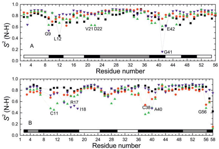
N-H generalized order parameters, S², for (a) ProtG and (b) BPTI (symbols as in Fig. 5). The order parameters were calculated over a 2-ns window for the EW/MD simulations and a 6-ns window for the ISM/LD simulations (Order parameters were calculated using CHARMM¹⁵¹). Experimental values are taken from ref. 107 for ProtG and from Goldenberg (private communication) for BPTI.

On average, the ProtG order parameters calculated from residues in the α-helical and β-strand regions of the structure indicate less flexibility in comparison to the NMR structure [Fig 7(a)]. The large deviation of the order parameter in G41 calculated from the CMAP/LD simulation appears to be an artifact, possibly indicating that the new parameter set is not yet completely optimized (see also the next section). It also appears that the order parameters calculated from the CMAP/LD trajectory are on average larger than the corresponding values obtained from the PAR22/LD and EW/MD trajectories, indicating that for ProtG the CMAP/LD trajectory may be somewhat overly rigid and probably unrelated to the solvent model. Comparison of the results found here with other reports indicates overall similar behavior and accuracy.¹⁰³

In BPTI, the order parameters calculated from the simulated structures tend to be smaller than the values obtained from NMR,¹⁰⁸ and the large deviations are confined to the loop regions [Fig. 7(b)]. Note, however, that the largest deviations are exhibited by the PAR22/LD trajectory, which is probably due to its instability. Moreover, the order parameters of the EW/MD and CMAP/LD simulations of residues in the loop regions linked by the C14–C38 disulfide bridge are smaller than the measured values. Interestingly, the S² values calculated from the EW/MD calculation seem to be very close to the S² calculated by other authors^109,110 in 1-ns simulations starting from the X-ray structure, although the explicit solvent representations are quite different. Caution should be exercised, however, when comparing the calculated S²(H-N) parameter with their experimental values, because internal water molecules were removed from the simulations and may affect the backbone dynamics of certain residues (e.g., P8, Y10, T11, C14, C38, G37, K41, and N43, whose -HN groups are all H-bonded to crystallographic water molecules); note that these residues belong to the loops, which are also the most flexible regions of the protein and where most outliers in Fig. 7b are located.

The covariance among different regions of a protein can reveal the extent of correlated motion and can be used to analyze and compare trajectories for their reliability and similarity. In general, the motions of different regions of a protein are not correlated, but in some cases, such as among proximal residues or regions, as in domain– domain communication, the two segments move in concert with each other, either in the same direction (correlated) or in the opposite direction (anti-correlated). The magnitude of the correlation can be estimated from the covariance, i.e., Δr_i · Δr_j, where Δr = r − $\overline{r}$and $\overline{r}$ denotes the average of r at the centroid of the corresponding residue i or j.¹¹¹ The normalized cross-correlation function C(i, j) between residue i and j is given by

$$C(i,j)=\langle \mathrm{\Delta }{r}_i\cdot \mathrm{\Delta }{r}_j\rangle /\sqrt{\langle \mathrm{\Delta }{r}_i^2\rangle \langle \mathrm{\Delta }{r}_j^2\rangle }$$ (10)

where the angle brackets denote an ensemble average; C(i, j) = 1 or C(i, j) = −1 means completely coupled or anti-correlated motion.

The correlation matrices for the two proteins calculated from the trajectories are shown in Figure 8. For each protein, the EW/MD results were obtained over the last 2 ns, while the last 10 ns were used for the ISM/LD trajectories. The diagonal elements of the covariance matrix are the positional RMSF that converge in a fairly short time, as shown in Figure 1. The off-diagonal elements converge more slowly¹¹² so that comparison between the ISM/LD and EW/MD results needs to be applied with caution. This is because if the trajectory is too short artifactual correlations may be seen that have not had enough time to be averaged out. Note that in ProtG several anti-correlated regions seen in the EW/MD plot have disappeared in the ISM/LD plots, and the highly correlated regions have decreased. This is also true for the CMAP/LD plot of BPTI, but not for the PAR22/LD simulation of this protein. However, because the latter trajectory is unstable, it is not possible to interpret the significance of the various correlated or anti-correlated regions.

Fig. 8.

Residue–residue based map of correlated motions of ProtG and BPTI. Results from the EW/MD simulations are given in (a) for ProtG and in (c) for BPTI; results from the ISM/LD simulations are shown in (b) and (d) with the PAR22/LD represented in the upper triangle and the CMAP/LD in the lower triangle of each panel. Red and yellow indicate regions of positive correlation, and dark blue indicates regions of anti-correlation.

In general, for both proteins, the regions of positive correlation correspond to highly coupled motions of residues within the same helix and between neighboring strands. For each protein, the patterns of correlation vary to some extent between the different simulations. Specifically, for ProtG the EW/MD simulation exhibits patterns of strong anti-correlations between the α-helix and the β-sheet, as well as between loop 19–22 and loop 47–50 [cf. Fig. 8(a)]. However, in both ISM/LD simulations [cf. Fig. 8(b); see caption] the anti-correlated motions between the α-helix and the β-sheet are much weaker, while anti-correlated motions between residues 9–12 and 37–41 in the ISM/LD simulations are not observed in the EW/MD plot. Note also the strong correlation seen between the two termini regions in all simulations. A strong correlation is also seen between Gly41 and the N-terminus in the CMAP/LD plot. This correlation is not present in either the EW/MD or PAR22/LD cross-correlation plots. These differences are probably related to the difference between PAR22 and CMAP potentials.

For BPTI, strongly coupled correlations are observed in the region close to the C14–C38 disulfide-bridge [cf. Fig. 8(c and d)]. All simulations predicted coupled motion between N-terminal helix 3–6 and the loop 36–44, and anti-correlated motion between the loop 25–28 and the C-terminal helix 48–55. The coupled motions between loops 8–17 and 36–44 and anti-correlated motion between the two helices are predicted by the EW/MD [cf. Fig. 8(c)] and PAR22/LD [cf. Fig. 8(d); see caption], but are probably artifactual because the EW/MD trajectory is too short and the PAR22/LD simulation is unstable. Results from an earlier study of cross correlations show reasonable agreement in the location of the correlated and anti-correlated regions.¹¹¹

Hydrogen Bonding

Protein HB patterns represent one of the most important structural features that characterize both secondary and tertiary structural motifs. It is therefore important to verify whether the experimentally observed HB patterns are reasonably preserved in long simulations, especially when implicit solvent models are used. In particular, the inter-residue HB characteristics of solvent-exposed residues may be strongly modified by the absence of explicit solvent. For the analysis of the simulations reported here, HB was identified using the criteria that the PA––H-PD (PA = proton acceptor; PD = proton donor) angle was ≥ 135° and that the PA––H bond length was ≤2.5 Å. Intra-residue HB and nearest-neighbor (i, i + 1) HB between main-chain PA and PD were excluded. The H-bonds are classified as b–b (backbone–backbone), b–sc (backbone–side chain) and sc–sc (side chain–side chain) corresponding, respectively, to the cases in which both PA and PD atoms belong to the backbone, one belongs to the backbone and the other to a side chain, and both belong to side chains, regardless of the atom types involved.

The numbers of H-bonds in each class, as observed in the crystal and in the average structures obtained in the simulations, are listed in Table IV. The results show that for all classes the numbers of H-bonds observed in the simulated structures agree well with the crystal structures except for the sc–sc type in the two ISM/LD simulations of ProtG. The number of b–b H-bonds found in ProtG is close to the reported value of 34 from experiments¹¹³ and from QM calculations.¹¹⁴ In BPTI, the number of b–b H-bonds in the simulations is in good agreement with the b–b HB found experimentally in native BPTI crystals¹¹⁵ and in earlier EW simulations.¹¹⁶

TABLE IV.

Number of H-Bonds Observed in Crystals and in Average Structures From Simulations of ProtG and BPTI

	ProtG				BPTI
H-bond Typea	Crystal	EW/MD	PAR22/LD	CMAP/LD	Crystal	EW/MD	PAR22/LD	CMAP/LD
B–b	32	29	30	32	22	20	21	20
B–sc	10	11	10	10	13	10	13	10
Sc–sc	11	12	2	3	4	2	2	2

^aH-bonds are specified as follows: both PD and PA in the backbone (b–b), one (PD or PA) in the backbone and the other in the side chain (b–sc), and both PD and PA atoms in side chains (sc–sc).

The extent of exact pairing correspondence to the crystal structure between PA and PD residues calculated from the average structures of the different simulations and crystal structure b–b type HB is >90% for ProtG and in BPTI it is about 70% for the ISM/LD average structures and 85% for the EW/MD average structure. In both proteins, the best correspondence is found from the EW/MD simulation.

For HB involving side-chain atoms, the number of b–sc HB-bonds of the calculated structures agrees quite well with the corresponding crystal structure (Table IV), and the extent of exact correspondence of the PA and PD between calculated and observed HB lies between 30 and 80%. Good correspondence is also noted for the four sc–sc type HB in BPTI for all simulations and for the EW/MD average structure of ProtG (70%). In contrast, the PAR22/LD and CMAP/LD structures of ProtG have lost most of the sc–sc H-bonds observed in the crystal or EW/MD structures. The residues involved in sc–sc HB are primarily on the surface of the protein with high solvent exposure (>50%), so it is not surprising that these residues are the most affected by the replacement of explicit with implicit solvent. In all of these cases, the conformations of the side chains have changed, increasing the PA––H separation beyond the threshold value of 2.5 Å (from about 3 to 6 Å as measured in the average structures). Nevertheless, the solvent exposure of these residues in the ISM/LD average structures of ProtG do not change much from the crystal structure values (see next section) suggesting that it might be the weakening of energies of these H-bonds that leads to their loss in the ISM/LD simulations (see discussion section and ref. 43).

Solvent Accessibility and pH-Dependent Properties

Insight into structural properties such as hydrophobic packing or potential modulating effects arising from the protein local environment can be obtained from the residue solvent exposures. The solvent-exposed fractions of the side chains are shown in Figure 9(a) for ProtG and in Figure 9(b) for BPTI. Inspection of Figure 9 shows that the side-chain exposed fractions (SCEF) of both the EW/MD and ISM/LD average structures closely follow the SCEF of the crystal structure. The deeply buried hydrophobic core in each protein was well preserved throughout the entire simulation for all solvent models and parameter sets. The SCEF calculated from the CMAP/LD simulations have the smallest RMSD from the crystal structure (see Table III). A few exceptions are noted where the different simulations indicate diverging degrees of burial or exposure, and the larger of these deviations are indicated in each plot. (Here the same threshold is used as in Table II to differentiate between buried and exposed residues. Note also that for the sake of completeness glycine SCEF were calculated from the hydrogens bonded to C_α, but they are not considered further in the analysis.)

Fig. 9.

Solvent-exposed fractions of side chains calculated from the average structures of (a) ProtG and (b) BPTI (symbols as in Fig. 5). The average structures were calculated from the last 2 ns of the EW/MD simulation and the last 6 ns of the ISM/LD simulations.

For ProtG, the RMSD of the average structure SCEF values from the crystal structure values are all small (see Table III), and scatter plots (not shown) of the calculated versus the crystal structure SCEF are strongly correlated (r >0.9). In ProtG [cf. Fig. 9(a)], only two residues, Leu12 and Gln35, show large differences between the average structures and the crystal structure SCEF: all simulations predict Leu12 to be solvent exposed, while in the crystal structure this residue is buried, whereas Gln35 in the PAR22/LD structure is buried while the others are solvent exposed.

The RMSD of the calculated SCEF from the crystal structure of BPTI are somewhat larger for the EW/MD and PAR22/LD simulations, but the CMAP/LD simulation is closer to the crystal structure (Table III). The CMAP/LD (vs. the crystal structure SCEF) scatter plot exhibits a correlation of 0.93, while the other two have a correlation of about 0.8. For BPTI [cf. Fig. 9(b)], there are a few divergent residues: Phe4 becomes solvent exposed in the average structures from the ISM/LD trajectories, but in both the crystal and the EW/MD average structures this residue is buried; note also two residues in loop1 where the EW SCEF are substantially larger than the SCEF calculated from the other structures; other residues in BPTI that exhibit diverging degrees of solvent exposure include C14 and C38.

Titratable residues that exhibit large shifts in their pKa values are often associated with protein function.^117–124 Thus the ability to estimate these pKa and reveal the microscopic origins of the observed shifts is of great interest. It has been observed that the incorporation of protein flexibility into the calculation of pKa increases their reliability,¹²⁵ and here the ability of the simulations reported in this work to provide reliable estimates of pKa values is analyzed (see Discussion). The calculations were carried out using the Microenvironment-Modulated_SCP approximation (MM_SCP).^97,98 The pKa values of all the titratable groups in ProtG and BPTI were calculated in two ways: (i) the pKa were first calculated from each of 600 structures extracted from the last 6 ns (ISM/LD trajectories) and 2 ns (EW/MD trajectories) and then averaged; and (ii) the pKa values were first calculated from the average structures used in the analyses discussed above. Table V gives the RMSD of all the calculated pKa values from the corresponding experimental values (the individual values can be obtained as Supplementary Material).

TABLE V.

RMSD of pKa Values of Titratable Residues in ProtG and BPTI Calculated From Trajectories

	ProtG				BPTI
Structure	Crystalc	EW/MD	PAR22/LD	CMAP/LD	Crystalc	EW/MD	PAR22/LD	CMAP/LD
RMSDa	0.58	0.38	0.45	0.39	0.36	0.36	0.34	0.30
RMSDb		0.36	0.47	0.44		0.30	0.41	0.33

References for RMSD calculations are experimental pKa’s.

^aObtained as an average over 600 pKa values calculated from the conformations generated over the last 2 ns (EW/MD) and last 6 ns (ISM/LD) of each trajectory.

^bObtained from each of the average structures calculated in the simulations; average structures obtained from the last 2 ns (EW/MD) and last 6 ns (ISM/LD) of the simulations (see text).

^cCrystal structure value is the average from three sources.⁹⁷,¹²⁵,¹⁵⁰

The results shown in Table V indicate that for most cases approach (i) described above yields pKa values with slightly smaller RMSD than approach (ii). While this result is not surprising, evidence has been presented that a carefully prepared average structure can give nearly equivalent quality results at a substantial reduction in required computing time.¹²⁶ In the present applications, the results given in Table V show that the pKa values calculated from the average structures obtained from the simulations yield pKa values with overall RMSD close to those obtained with method (i). Compared to the pKa values calculated from the crystal structure, there appears to be a trend toward smaller errors in the pKa values calculated from both EW and ISM simulations. This finding suggests that incorporation of flexibility from implicit solvent simulations is as effective in improving pKa calculations as simulations with explicit solvent. One caveat needs to be noted: in the systems studied here all of the titratable residues are solvent exposed and their pKa do not undergo large shifts from their solution values. Therefore the improvements found in BPTI and ProtG may not be observed in cases in which the titratable residue is deeply buried and its pKa value is strongly shifted.

Discussion

ProtG, BPTI, and Ubq have been studied in the past using experimental and theoretical methods. They are among the best-characterized proteins and detailed information on their structure, dynamics, and thermodynamic properties is available.^{95,99,103,107–109,111,127–133} The calculations reported in this article in particular explored the ability of the SCP-based continuum model to provide stable trajectories of lengths 30–40 ns and the ability to conserve the HB pattern of exposed side chains, when applied in combination with atomistic descriptions of the solute. Overall, the properties calculated with this continuum representation of the solvent agree well with the corresponding experimental values and are also in reasonable agreement with results from explicit water simulations. The differences in the calculated properties are slightly smaller for ProtG than for BPTI, which might be due to the greater rigidity of the former protein, as also evidenced by the greater stability of its trajectories. It was also seen that the structural integrity, especially of the cores of each protein, was well conserved. It is noted that with the exception of the energetics of sc–sc HB, the parameterization of the SCP–ISM used in the calculations was the same as has been used in all earlier reports (see Discussion in refs. ^8,34, and ⁶⁴).

The distortion of the BPTI structure from the PAR22/LD simulation supports the need for longer simulations when exploring the stability of trajectories. In the present case, the PAR22/LD simulation began to denature after about 3 ns, with further distortions at ~ 15 ns, but simulations started with different initial conditions can remain stable much longer (unpublished results), although the same features of the instability discussed herein are still observed. An intriguing question resulting from the analysis of the main-chain torsion angles concerns the stability of the EW/MD simulation. The inability of PAR22 to access the α_L region seems to be responsible for the deviation of the (φ,φ) values of R39 and, perhaps the response of G36 to compensate for the distorted R39 conformation. Similar distortions of residues with backbone dihedral angles in the α_L-region were here observed in Ubq, as well as additional adjustments in other residues that may compensate to preserve the solution structure. Longer and possibly multiple EW/MD simulations would be required to properly explore this question. This study shows, however, that the CMAP in CHARMM may stabilize the dynamics of proteins in long simulations compared to PAR22, although some adverse effects were observed in the quality of the calculated order parameters (this seems to be unrelated to the absence of explicit solvent and may be related to the CMAP potential). Although more work is needed to validate both CMAP and the SCP–ISM, their combination seems to yield quite satisfactory results in all the structural and dynamical properties studied in this article.

Another issue related to the conformation of BPTI is that the crystal structure contains four water molecules located in the vicinity of the disulfide-bridged loops.^134,135 These water molecules have residence times in the nanosecond to the millisecond range^136,137 and have not been introduced in the ISM/LD calculations, although they were not explicitly introduced in the EW/MD either for the sake of comparison. It is noted that the use of a continuum representation of the solvent should not preclude the inclusion of individual water molecules in the system. In this case, the individual molecules (e.g., crystallographic water molecules) would have to be treated as part of the solute. However, although the solvation energy of individual water molecules can be reasonably described by a continuum model such as the SCP–ISM, other questions have to be addressed such as the correct water–sc HB interaction energies, which may be critical to reproduce experimentally determined residence times in a LD simulation (SAH, unpublished results). It is noted that, in this case, a proper LD algorithm is essential and would contribute to maintaining the individual water molecules confined in the protein interior. Therefore, a refinement of the simple LD algorithm used here is needed to mimic anisotropic pressure and random collision from outside the protein only (SAH, unpublished results). Besides, a protocol should be designed to mimic the penetration of a water molecule or ion to a protein cavity once they diffuse out of the protein.

The behavior of solvent-exposed side chains in the dynamics reported here seems to be controlled mainly by the quality of the continuum model, including hydrophobic, electrostatic, and HB interactions, and is probably less affected by improvements of the rest of the force field, i.e., in the atomistic description of the solute (e.g., CMAP over PAR22). The fundamental relevance of correctly describing HB energetics in a continuum model has been discussed previously^43,63 (see also Introduction). The description of HB in the SCP–ISM version used in the calculations reported here needs further refinement, as evidenced by the loss of sc–sc H-bonds in the two ISM/LD simulations of ProtG but not in the EW/MD simulation. A further refinement of the model would contain a more accurate HB description based on a parameterization obtained from systematic potentials of mean force calculations in EW/MD simulations.⁴³ This new development would extend the limits of application of the continuum model to problems in which sc–sc interactions play a central role such as in ligand-binding and protein–protein interactions. Therefore, this refinement is important for dynamics simulations of dimers and other macromolecular complexes, because HB interactions may be critical for the stability of the interface.

The pKa values calculated from the trajectories support the idea that incorporation of protein flexibility improves the results. Since the MM–SCP is a variational approach that partially accounts for structural responses (relaxation) to changes in the electrostatic configuration of the system, the improvements noted here are due to the instantaneous structural changes described by the fluctuations. Thus the improvements noted in Table V, which in the present calculations are larger in ProtG than in BPTI, suggests that the simulations present a fairly realistic description of the (temperature-dependent) fluctuations. At the same time, it needs to be recognized that methods like the MM–SCP that use partial charges (usually taken from a force field) to describe the electrostatic and solvation properties of the macromolecule are limited in their reliability and ability to reveal the underlying physics that control properties like acid-base equilibrium constants. This is so because they cannot describe the detailed electronic structure that actually determines molecular properties, including pKa. Such a complete description (depending on electronic structure) can only be obtained using QM methods. Such approaches are being explored,^138,139 but because of the computational demands progress in the use of QM approaches has been slow.

The study reported in this paper is timely and relevant because doubts exist concerning the ability of continuum models of solvation to describe structural and dynamical properties of biomolecules (e.g., see refs. ^140–142). Clarifying this issue is essential if there is any hope of addressing more challenging issues such as structure–dynamics–function relationships in biomolecules. Simple models of molecular energetics have been traditionally used to understand general physical principles behind specific processes (e.g., lattice model potentials to study folding kinetics and dynamics, or Lennard–Jones sphere potentials to gain insight into properties of liquids).^143–149 Many problems in biology, however, require a level of accuracy that can only be attained with a focused and persistent effort in the development of better computational approaches. Thus, more accurate atomistic force fields for the solute and more realistic continuum models of solvent effects⁶² would probably expand the possibilities of applying computational techniques to biology-related problems and to overcome the limitations of current methodologies. Structure predictions, analysis of protein folding kinetics and dynamics, protein–protein association, protein–ligand interactions, etc, are all important and exciting problems that can be addressed with atomistic/continuum models. The insight gained from these studies may have deep biological implications and also generate hypotheses on the function of these systems. Unfortunately, much more elementary and less exciting problems and basic questions still remain to be investigated, such as the capability of a continuum model (a force field in general) to generate stable trajectories in long time regimes (i.e., of biological significance), to describe the conformations and dynamics of solvent-exposed side chains, or to properly represent and preserve the HB network throughout the system. All three questions have been addressed in this work. Failure to describe these basic properties in a quantitatively satisfactory way would render the approximation useless and raise doubts about its reliability in the most challenging and ambitious applications mentioned above.

Finally, it is noted that many processes in macromolecules are controlled not only by electrostatics and HB interactions, but thermodynamic-related phenomena such as hydrophobicity and other solvent-induced forces^152–155 also play important roles in many cases. For the calculations reported here, a simple cavity term was used, which is proportional to the total SASA of the molecule. This simplistic description is far from a comprehensive hydrophobic model that can be used reliably in biological problems or in simulations of polymers in general (see Discussion in ref. 8). Non-electrostatic solvent-induced forces (e.g., hydrophobicity) may have an effect on the dynamics and conformations of solvent-exposed side chains that remains to be investigated in the context of the SCP–ISM. Another problem that remains to be resolved is the effect of salts, which are ubiquitous in biological systems. The LDS method described in Materials and Methods, upon which the SCP–ISM is based, allows for a formal description of the screening due to an ion atmosphere around point charges or dipoles and may provide a simple way to describe salt effects in a continuum model for computer calculations (SAH unpublished).

The current version of the SCP–ISM has been implemented in CHARMM (version c31b1) for use in combination with an atomistic description of the solute (PAR22 or CMAP); see ref. 64 for a summary of the implementation details. As currently implemented, the SCP–ISM is about two to three times slower (depending on platform and compilation options) than the corresponding vacuum calculation.

References

- 1.Rahman A, Stillinger FH. Molecular dynamics study of liquid water. J Chem Phys. 1971;55:3336–3359. [Google Scholar]
- 2.Stillinger FH, Weber TA. Computer simulation of local order in condensed phases of silicon. Phys Rev B. 1985;31:5262–5271. doi: 10.1103/physrevb.31.5262. [DOI] [PubMed] [Google Scholar]
- 3.Allen MP, Tildesley DJ. Computer simulation of liquids. Oxford: Clarendon Press; 1987. [Google Scholar]
- 4.Car R, Parrinello M. Unified approach for molecular dynamics and density-functional theory. Phys Rev Lett. 1985;55:2471. doi: 10.1103/PhysRevLett.55.2471. [DOI] [PubMed] [Google Scholar]
- 5.Matsumoto M, Saito S, Ohmine I. Molecular dynamics simulation of the ice nucleation and growth process leading to water freezing. Nature. 2002;416:409–413. doi: 10.1038/416409a. [DOI] [PubMed] [Google Scholar]
- 6.Karplus M, McCammon JA. Molecular dynamics simulations of biomolecules. Nature Structural Biology. 2002;9:646–652. doi: 10.1038/nsb0902-646. [DOI] [PubMed] [Google Scholar]
- 7.Geissler PL, Dellago C, Chandler D, Hutter J, Parrinello M. Autoionization in liquid water. Science. 2001;291:2121–2124. doi: 10.1126/science.1056991. [DOI] [PubMed] [Google Scholar]
- 8.Hassan SA, Mehler EL, Zhang D, Weinstein H. Molecular dynamics simulations of peptides and proteins with a continuum electrostatic model based on screened coulomb Potentials. Proteins. 2003;51:109–125. doi: 10.1002/prot.10330. [DOI] [PubMed] [Google Scholar]
- 9.TenWolde PR, Chandler D. Drying induced hydrophobic polymer collapse. Proc Nat Acad Sci USA. 2002;99:6539–6543. doi: 10.1073/pnas.052153299. [DOI] [PMC free article] [PubMed] [Google Scholar]
- 10.Cheatham TE, Kollman P. Molecular dynamics simulation of nucleic acids. Ann Rev Phys Chem. 2000;51:435. doi: 10.1146/annurev.physchem.51.1.435. [DOI] [PubMed] [Google Scholar]
- 11.Warshel A, Levitt M. Theoretical studies of enzymic reactions: dielectric, electrostatic and steric stabilization of the carboniom ion in the reaction of lysozyme. J Mol Biol. 1976;103:227–249. doi: 10.1016/0022-2836(76)90311-9. [DOI] [PubMed] [Google Scholar]
- 12.Singh UC, Kollman PA. A combined ab initio quantum mechanical and molecular mechanical method for carrying out simulations on complex molecular systems: applications to the CH3Cl+Cl− exchange reaction and gas phase protonation. J Comp Chem. 1986;7:718. [Google Scholar]
- 13.Field MJ, Bash PA, Karplus M. A combined quantum mechanical and molecular mechanical potential for molecular dynamics simulations. J Comp Chem. 1990;11:700–733. [Google Scholar]
- 14.Feig M, Brooks CL. Recent advances in the development and application of implicit solvent models in biomolecule simulations. Curr Op Struc Biol. 2004;14:217–224. doi: 10.1016/j.sbi.2004.03.009. [DOI] [PubMed] [Google Scholar]
- 15.Hassan SA, Guarnieri F, Mehler EL. A general treatment of solvent effects based on screened coulomb potentials. J Phys Chem B. 2000;104:6478–6489. [Google Scholar]
- 16.Tomasi J, Perisco M. Molecular interactions in solution: an overview of methods based on continuous distribution of the solvent. Chem Revs. 1994;94:2027–2094. [Google Scholar]
- 17.Orozco M, Luque FJ. Theoretical methods for the description of the solvent effect in biomolecular systems. Chem Rev. 2000;100:4187. doi: 10.1021/cr000703z. [DOI] [PubMed] [Google Scholar]
- 18.Simonson T. Macromolecular electrostatics: continuum models and their growing pains. Curr Opin Struct Biol. 2001;11:243–252. doi: 10.1016/s0959-440x(00)00197-4. [DOI] [PubMed] [Google Scholar]
- 19.Lazaridis T, Karplus M. Effective energy function for proteins in solution. Proteins. 1999;35:133–152. doi: 10.1002/(sici)1097-0134(19990501)35:2<133::aid-prot1>3.0.co;2-n. [DOI] [PubMed] [Google Scholar]
- 20.Cramer CJ, Truhlar DG. Implicit solvation models: equilibria, structure, spectra, and dynamics. Chem Revs. 1999;1999:2161–2200. doi: 10.1021/cr960149m. [DOI] [PubMed] [Google Scholar]
- 21.Surjan PR, Naray-Szabo G, editors. Molecular embedding. J Math Chem. 1992;(Special issue):10. [Google Scholar]
- 22.Warshel A, Aqvist J. Electrostatic energy and macromolecular function. Annu Rev Biophys Biophys Chem. 1991;20:267–298. doi: 10.1146/annurev.bb.20.060191.001411. [DOI] [PubMed] [Google Scholar]
- 23.Sharp KA, Honig B. Electrostatic interactions in macromolecules: theory and applications. Annu Rev Biophys Biophys Chem. 1990;19:301–332. doi: 10.1146/annurev.bb.19.060190.001505. [DOI] [PubMed] [Google Scholar]
- 24.Chothia C. Hydrophobic bonding and accessible surface area in proteins. Nature. 1974;248:338–339. doi: 10.1038/248338a0. [DOI] [PubMed] [Google Scholar]
- 25.Baldwin RL. Making a network of hydrophobic clusters. Science. 2002;295:1657. doi: 10.1126/science.1069893. [DOI] [PubMed] [Google Scholar]
- 26.Jeffrey GA, Saenger W. Hydrogen bonding in biological structures. Heidelberg: Springer-Verlag; 1991. [Google Scholar]
- 27.Baker EN, Hubbard RE. Hydrogen bonding in globular proteins. Prog Biophys Molec Biol. 1984;44:97–179. doi: 10.1016/0079-6107(84)90007-5. [DOI] [PubMed] [Google Scholar]
- 28.Fersht AR, Shi J-P, Knill-Jones J, Lowe DM, Wilkinson AJ, Blow DM, Brick P, Carter P, Waye MM, Winter G. Hydrogen bonding and biological specificity analysed by protein engineering. Nature. 1985;314:235–238. doi: 10.1038/314235a0. [DOI] [PubMed] [Google Scholar]
- 29.Cohen BE, McAnaney TB, Park ES, Jan YN, Boxer SG, Jan LY. Probing protein electrostatics with a synthetic fluorescent amino acid. Science. 2002;296:1700. doi: 10.1126/science.1069346. [DOI] [PubMed] [Google Scholar]
- 30.Warshel A, Russell ST. Calculation of electrostatic interactions in biological systems and in solutions. Quart Rev Biophys. 1984;17:283–422. doi: 10.1017/s0033583500005333. [DOI] [PubMed] [Google Scholar]
- 31.Warshel A, Papazyan A. Electrostatic effects in macromolecules: fundamental concepts and practical modeling. Curr Opin Struct Biol. 1998;8:211–217. doi: 10.1016/s0959-440x(98)80041-9. [DOI] [PubMed] [Google Scholar]
- 32.Papazyan A, Warshel A. Effect of solvent discreteness on solvation. J Phys Chem B. 1998;102:5348. [Google Scholar]
- 33.Schutz CN, Warshel A. What are the dielectric “constants” of proteins and how to validate electrostatic models? Proteins. 2001;44:400–417. doi: 10.1002/prot.1106. [DOI] [PubMed] [Google Scholar]
- 34.Hassan SA, Mehler EL. A critical analysis of continuum electrostatics: the screened Coulomb potential-implicit solvent model and the study of the alanine dipeptide and discrimination of misfolded structures of proteins. Proteins. 2002;47:45–61. doi: 10.1002/prot.10059. [DOI] [PubMed] [Google Scholar]
- 35.Lum K, Chandler D, Weeks JD. Hydrophobicity at small and large length scales. J Phys Chem B. 1999;103:4570. [Google Scholar]
- 36.Chandler D. Two faces of water. Nature. 2002;417:491. doi: 10.1038/417491a. [DOI] [PubMed] [Google Scholar]
- 37.Dill KA. The meaning of hydrophobicity. Science. 1990;250:297. doi: 10.1126/science.2218535. [DOI] [PubMed] [Google Scholar]
- 38.Hummer G, Garde S, Garcia AE, Paulaitis ME, Pratt EA. Hydrophobic effects on a molecular scale. J Phys Chem B. 1998;102:10469. [Google Scholar]
- 39.Hummer G, Garde S, Garcia AE, Pratt EA. New perspectives on hydrophobic effects. Chem Phys. 2000;258:349. [Google Scholar]
- 40.Hyun J-K, Ichiye T. Nonlinear response in ionic solvation: a theoretical investigation. J Chem Phys. 1998;109:1074–1083. [Google Scholar]
- 41.Bader RFW, Larouche A, Gatti C, Carroll MT, MacDougall PJ, Wiberg KB. Properties of atoms in molecules: dipole moments and transferability of properties. J Chem Phys. 1987;87:1142–1152. [Google Scholar]
- 42.Bader RFW. A quantum theory of molecular structure and its applications. Chem Rev. 1991;91:893–928. [Google Scholar]
- 43.Hassan SA. Intermolecular potentials of mean force of amino acid side chains interactions in aqueous medium. J Phys Chem B. 2004;50:19501. [Google Scholar]
- 44.Webb TJ. The free energy of hydration of ions and the electrostriction of the solvent. J Am Chem Soc. 1926;48:2589–2603. [Google Scholar]
- 45.Debye P, Pauling L. The inter-ionic attraction theory of ionized solutes. IV. The influence of variation of dielectric constant on the limiting law for small concentrations. J Am Chem Soc. 1925;47:2129–2134. [Google Scholar]
- 46.Schwarzenbach G. Der Einfluss einer Ionenladung auf die Acidität einer Säure. Z Physik Chem A. 1936;176:133–153. [Google Scholar]
- 47.Harvey SC, Hoekstra P. Dielectric relaxation spectra of water adsorbed on lysozyme. J Phys Chem. 1972;76:2987–2994. doi: 10.1021/j100665a011. [DOI] [PubMed] [Google Scholar]
- 48.Pennock BD, Schwan HP. Further observations on the electrical properties of hemoglobin-bound water. J Phys Chem. 1969;73:2600–2610. doi: 10.1021/j100842a024. [DOI] [PubMed] [Google Scholar]
- 49.Takashima S, Schwan HP. Dielectric dispersion of crystalline powders of amino acids, peptides and proteins. J Phys Chem. 1965;69:4176–4182. doi: 10.1021/j100782a019. [DOI] [PubMed] [Google Scholar]
- 50.Hasted JB, Ritson DM, Collie CH. Dielectric properties of aqueous ionic solutions. Parts I and II. J Chem Phys. 1948;16:1–21. [Google Scholar]
- 51.Ehrenson S. Continuum radial dielectric functions for ion and dipole solution systems. J Comp Chem. 1989;10:77–93. [Google Scholar]
- 52.Bucher M, Porter TL. Analysis of the Born model for hydration of ions. J Phys Chem. 1986;90:3406–3411. [Google Scholar]
- 53.Debye P. Polar molecules. New York: Dover; 1929. [Google Scholar]
- 54.Lorentz HA. Theory of electrons. New York: Dover; 1952. [Google Scholar]
- 55.Sack VH. The dielectric constant of electrolytes. Phys Z. 1926;27:206–208. [Google Scholar]
- 56.Sack VH. The dielectric constants of solutions of electrolytes at small concentrations. Phys Z. 1927;28:199–210. [Google Scholar]
- 57.Onsager L. Electric moments of molecules in liquids. J Amer Chem Soc. 1936;58:1486–1493. [Google Scholar]
- 58.Mehler EL. The Lorentz-Debye-Sack theory and dielectric screening of electrostatic effects in proteins and nucleic acids. In: Murray JS, Sen K, editors. Molecular electrostatic potential: concepts and applications. Vol. 3. Amsterdam: Elsevier Science; 1996. pp. 371–405. [Google Scholar]
- 59.Stone AJ. Distributed multipole analysis, or how to describe a molecular charge distribution. Chem Phys Lett. 1981;83:233–239. [Google Scholar]
- 60.Bader RFW. Atoms in molecules. Acc Chem Res. 1985;18:9–15. [Google Scholar]
- 61.Stone AJ, Alderton M. Distributed multipole analysis: methods and applications. Mol Phys. 2002;100:221–233. [Google Scholar]
- 62.Hassan SA, Mehler EL. From quantum chemistry and the classical theory of polar liquids to continuum approximations in molecular mechanics calculations. Int J Quant Chem. 2005;102:986. [Google Scholar]
- 63.Hassan SA, Guarnieri F, Mehler EL. Characterization of hydrogen bonding in a continuum solvent model. J Phys Chem B. 2000;104:6490–6498. [Google Scholar]
- 64.Hassan SA. http://cmm.cit.nih.gov/~mago/SCPISM.html.
- 65.Mehler EL, Eichele E. Electrostatic effects in water-accessible regions of proteins. Biochemistry. 1984;23:3887–3891. [Google Scholar]
- 66.Jackson JD. Classical electrodynamics. New York: Wiley; 1975. [Google Scholar]
- 67.Born M. Volumen und Hydrationswärme der Ionen. Z Phys. 1920;1:45–48. [Google Scholar]
- 68.Mehler EL, Periole X, Hassan SA, Weinstein H. Key issues in the computational simulation of GPCR function: representation of loop domains. J Comp Aided Mol Design. 2002;16:841–853. doi: 10.1023/a:1023845015343. [DOI] [PubMed] [Google Scholar]
- 69.Hassan SA, Mehler EL, Weinstein H. Structure calculations of protein segments connecting domains with defined secondary structure: a simulated annealing Monte Carlo combined with biased scaled collective variables technique. In: Hark K, Schlick T, editors. Lecture notes in computational science and engineering. Vol. 24. New York: Springer Verlag, Ag.; 2002. pp. 197–231. [Google Scholar]
- 70.Hassan SA, Guarnieri F, Mehler EL. A general treatment of solvent effects based on screened Coulomb potentials. J Phys Chem B. 2000;104:6478–6489. [Google Scholar]
- 71.Quiocho FA, Sack JS, Vyas NK. Stabilization of charges on isolated ionic groups sequestered in proteins by polarized peptide units. Nature. 1987;329:561–564. doi: 10.1038/329561a0. [DOI] [PubMed] [Google Scholar]
- 72.Lesser GJ, Rose GD. Hydrophobicity of amino-acid subgroups in proteins. Proteins. 1990;8:6–13. doi: 10.1002/prot.340080104. [DOI] [PubMed] [Google Scholar]
- 73.Pace CN. Polar group burial contributes more to protein stability than nonpolar group burial. Biochemistry. 2001;40:310–313. doi: 10.1021/bi001574j. [DOI] [PubMed] [Google Scholar]
- 74.Pace CN, Horn G, Hebert EJ, Bechert J, Shaw K, Urbanikova L, Scholtz JM, Sevcik J. Tyrosine hydrogen bonds make a large contribution to protein stability. J Mol Bio. 2001;312:393–404. doi: 10.1006/jmbi.2001.4956. [DOI] [PubMed] [Google Scholar]
- 75.Pace CN. Energetics of biological macromolecules. Vol. 259. Methods in Enzymology; 1995. Evaluating contribution of hydrogen bonding and hydrophobic bonding to protein folding; pp. 538–554. [DOI] [PubMed] [Google Scholar]
- 76.Myers JK, Pace CN. Hydrogen bonding stabilizes globular proteins. Biophys J. 1996;71:2033–2039. doi: 10.1016/S0006-3495(96)79401-8. [DOI] [PMC free article] [PubMed] [Google Scholar]
- 77.Giletto A, Pace CN. Buried, charged, non-ion paired aspartic acid 76 contributes favorably to the conformational stability of ribonucluease. Biochemistry. 1999;38:13379–13384. doi: 10.1021/bi991422s. [DOI] [PubMed] [Google Scholar]
- 78.Takano K, Scholtz JM, Sacchettini JC, Pace CN. The contribution of polar group burial to protein stability is strongly context-dependent. J Biol Chem. 2003;278:31790–31795. doi: 10.1074/jbc.M304177200. [DOI] [PubMed] [Google Scholar]
- 79.Honig B, Cohen FE. Adding backbone to protein folding: why proteins are polypeptides. Folding & Design. 1996;1:R17–R20. doi: 10.1016/S1359-0278(96)00005-3. [DOI] [PubMed] [Google Scholar]
- 80.Nicholls A, Sharp KA, Honig B. Protein folding and association: insights from the interfacial and thermodynamic properties of hydrocarbons. Proteins. 1991;11:281–296. doi: 10.1002/prot.340110407. [DOI] [PubMed] [Google Scholar]
- 81.Fersht A. Enzyme structure and mechanism. New York: W.H. Freedman & Co.; 1985. [Google Scholar]
- 82.Sankararamakrishnan R, Konvicka K, Mehler EL, Weinstein H. Solvation in simulated annealing and high temperature molecular dynamics of proteins: a restrained water droplet model. Int J Quant Chem. 2000;77:174–186. [Google Scholar]
- 83.Brooks BR, Bruccoleri RE, Olafson BD, States DJ, Swaminathan S, Karplus M. CHARMM: A program for macromolecular energy, minimization and dynamics calculations. J Comp Chem. 1983;4:187–217. [Google Scholar]
- 84.MacKerell AD, Bashford D, Bellott M, Dunbrack RL, Evanseck JD, Field MJ, Fischer S, Gao J, Guo H, Ha S, Joseph-McCarthy D, Kuchnir L, Kuczera K, Lau FTK, Mattos C, Michnick S, Ngo T, Nguyen DT, Prodhom B, Reiher WE, Roux B, Schlenkrich M, Smith JC, Stote R, Straub J, Watanabe M, Wiorkiewicz-Kuczera J, Yin D, Karplus M. All-atom empirical potential for molecular modeling and dynamics studies of proteins. J Phys Chem B. 1998;102:3586–3616. doi: 10.1021/jp973084f. [DOI] [PubMed] [Google Scholar]
- 85.Shen MY, Freed KF. Long time dynamics of met-enkephalin: comparison of explicit and implicit solvent models. Biophys J. 2002;82:1791. doi: 10.1016/s0006-3495(02)75530-6. [DOI] [PMC free article] [PubMed] [Google Scholar]
- 86.Pastor RW, Karplus M. Parameterization of the friction constant for stochastic simulations of polymers. J Phys Chem. 1988;92:2636–2641. [Google Scholar]
- 87.Feig M, MacKerell AD, Brooks CL. Force field influence on the observation of pi-helical protein structures in molecular dynamics simulations. J Phys Chem B. 2003;107:2831–2836. [Google Scholar]
- 88.MacKerell AD, Jr, Feig M, Brooks CL., III Improved treatment of the protein backbone in empirical force fields . J Am Chem Soc. 2004;126:698–699. doi: 10.1021/ja036959e. [DOI] [PubMed] [Google Scholar]
- 89.MacKerell JAD, Bashford D, Bellott M, Dunbrack RL, Jr, Evanseck JD, Field MJ, Fischer S, Gao J, Guo H, Ha S, Joseph-McCarthy D, Kuchnir L, Kuczera K, Lau FTK, Mattos C, Michnick S, Ngo T, Nguyen DT, Prodhom B, Reiher WE, Roux B, Schlen-krich M, Smith JC, Stote R, Straub J, Watanabe M, Wiorkiewicz-Kuczera J, Yin D, Karplus M. All-atom empirical potential for molecular modeling and dynamics studies of proteins. J Phys Chem B. 1998;102:3586–3616. doi: 10.1021/jp973084f. [DOI] [PubMed] [Google Scholar]
- 90.Smith PE. The alanine dipeptide free energy surface in solution. J Chem Phys. 1999;111:5568–5579. [Google Scholar]
- 91.Hu H, Elstner M, Hermans J. Comparison of a QM/MM force field and molecular mechanics force fields in simulations of alanine and glycine “dipeptides” (Ace-Ala-Nme and Ace-Gly-Nme) in water in relation to the problem of modeling the unfolded peptide backbone in solution. Proteins. 2003;50:451–463. doi: 10.1002/prot.10279. [DOI] [PubMed] [Google Scholar]
- 92.Sibanda BL, Blundell TL, Thornton JM. Conformation of β-hairpins in protein structures: a systematic classification with applications to modeling by homology electron density fitting and protein engineering. J Mol Biol. 1989;206:759–777. doi: 10.1016/0022-2836(89)90583-4. [DOI] [PubMed] [Google Scholar]
- 93.Ramirez-Alvardo M, Blanco FJ, Serrano L. De novo design and structural analysis of a model β-hairpin peptide system. Nat Struc Bio. 1996;3:604–612. doi: 10.1038/nsb0796-604. [DOI] [PubMed] [Google Scholar]
- 94.Gallagher T, Alexander P, Bryan P, Gilliland GL. Two crystal structures of the BI immunoglobulin-binding domain of streptococcal protein G and comparison with NMR. Biochemistry. 1994;33:4721–4729. [PubMed] [Google Scholar]
- 95.Gronenborn AM, Filpula DR, Essig NZ, Achari A, Whitlow M, Wingfield PT, Clore GM. A novel, highly stable fold of the immunoglobulin binding domain of streptococcal protein G. Science. 1991;253:657. doi: 10.1126/science.1871600. [DOI] [PubMed] [Google Scholar]
- 96.Marquart M, Deisenhofer J, Bode W, Huber R. The geometry of the reactive site and of the peptide groups in trypsin, trypsinogen and its complexes with inhibitors. Acta Crys Sect B. 1983;39:480. [Google Scholar]
- 97.Mehler EL, Guarnieri F. A self-consistent, microenvironment modulated screened Coulomb potential approximation to calculate pH dependent electrostatic effects in proteins. Biophysics J. 1999;77:3–22. doi: 10.1016/S0006-3495(99)76868-2. [DOI] [PMC free article] [PubMed] [Google Scholar]
- 98.Mehler EL. A self-consistent, free energy based approximation to calculate pH dependent electrostatic effects in proteins. J Phys Chem. 1996;100:16006–16018. [Google Scholar]
- 99.Vijay-Kumar S, Bugg CE, Cook WJ. Structure of Ubiquitin refined at 1.8Å resolution. J Mol Biol. 1987;194:531–544. doi: 10.1016/0022-2836(87)90679-6. [DOI] [PubMed] [Google Scholar]
- 100.Cornilescu G, Marquardt JL, Ottiger M, Bax A. Validation of protein structure from anisotropic carbonyl chemical shifts in a dilute liquid crystalline phase. J Am Chem Soc. 1998;120:6836–6837. [Google Scholar]
- 101.McCammon JA, Harvey SC. Dynamics of proteins and nucleic acids. New York: Cambridge University Press; 1987. [Google Scholar]
- 102.Hünenberger PH, Mark AE, Vangunsteren WF. Fluctuation and cross-correlation analysis of protein motions observed in nanosecond molecular dynamics simulations. J Mol Biol. 1995;252:492. doi: 10.1006/jmbi.1995.0514. [DOI] [PubMed] [Google Scholar]
- 103.Sheinerman FB, Brooks IIICL. A molecular dynamics simulation study of segment B1 of protein G. Proteins. 1997;29:193. doi: 10.1002/(sici)1097-0134(199710)29:2<193::aid-prot7>3.0.co;2-e. [DOI] [PubMed] [Google Scholar]
- 104.Chandrasekhar I, Cloreb G, Szabo A, Gronenborn A, Brook B. A 500 ps molecular dynamics simulation study of interleukin-1 beta in water: correlation with nuclear magnetic resonance spectroscopy and crystallography. J Mol Biol. 1992;226:239–250. doi: 10.1016/0022-2836(92)90136-8. [DOI] [PubMed] [Google Scholar]
- 105.Lipari G, Szabo A. Model-free approach to the interpretation of nuclear magnetic resonance relaxation in macromolecules. J Am Chem Soc. 1982;104:4546–4559. [Google Scholar]
- 106.Cavanagh J, Fairbrother WJ, Palmer AGI, Skelton NJ. Protein NMR spectroscopy: principles and practice. San Diego: Academic Press; 1996. [Google Scholar]
- 107.Barshi JJ, Jr, Grasberger B, Gronenborn AM, Clore GM. Investigation of the backbone dynamics of the IgG-binding domain of streptococcal protein G by heteronuclear two-dimensional 1H–15N nuclear magnetic resonance spectroscopy . Protein Sci. 1994;3:15. doi: 10.1002/pro.5560030103. [DOI] [PMC free article] [PubMed] [Google Scholar]
- 108.Beeser SA, Oas TG, Goldenberg DP. Determinants of backbone dynamics in native BPTI: cooperative influence of the 14–38 disulfide and the Tyr35 side-chain. J Mol Biol. 1998;284:1581–1596. doi: 10.1006/jmbi.1998.2240. [DOI] [PubMed] [Google Scholar]
- 109.Smith PE, van Schaik RC, Szyperski T, Wuthrich K, van Gunsteren WF. Internal mobility of the basic pancreatic trypsin inhibitor in solution: a comparison of NMR spin relaxation measurements and molecular dynamics simulations. J Mol Biol. 1995;246:356–365. doi: 10.1006/jmbi.1994.0090. [DOI] [PubMed] [Google Scholar]
- 110.Basdevant N, Borgis D, Ha-Duong T. A semi-implicit solvent model for the simulation of peptides and proteins. J Comp Chem. 2004;25:1015–1029. doi: 10.1002/jcc.20031. [DOI] [PubMed] [Google Scholar]
- 111.Ichiye T, Karplus M. Collective motions in proteins: a covariance analysis of atomic fluctuations in molecular dynamics and normal mode simulations. Proteins. 1991;11:205–217. doi: 10.1002/prot.340110305. [DOI] [PubMed] [Google Scholar]
- 112.Clarage JB, Romo T, Andrews BK, Pettitt BM. A sampling problem in molecular dynamics simulations of macromolecules. Proc Natl Acad Sci USA. 1995;92:3288–3292. doi: 10.1073/pnas.92.8.3288. [DOI] [PMC free article] [PubMed] [Google Scholar]
- 113.Cornilescu G, Ramirez BE, Frank MK, Clore GM, Gronenborn AM, Bax A. Correlation between 3hJNC′ and hydrogen bond length in proteins. J Am Chem Soc. 1999;121:6275–6279. [Google Scholar]
- 114.Barfield M. Structural dependencies of interresidue scalar coupling h3JNC′ and donor 1H chemical shifts in the hydrogen bonding regions of proteins. J Am Chem Soc. 2002;124:4158–4168. doi: 10.1021/ja012674v. [DOI] [PubMed] [Google Scholar]
- 115.Wlodawer A, Nachman J, Gilliland G, Gallagher W, Woodward C. Structure of form III crystals of bovine pancreatic trypsin inhibitor. J Mol Bio. 1987;198:469–480. doi: 10.1016/0022-2836(87)90294-4. [DOI] [PubMed] [Google Scholar]
- 116.Levitt M, Sharon R. Accurate simulation of protein dynamics in solution. Proc Natl Acad Sci USA. 1988;85:7557–7561. doi: 10.1073/pnas.85.20.7557. [DOI] [PMC free article] [PubMed] [Google Scholar]
- 117.Fersht AR. Conformational equilibria in alpha-chymotrypsin and delta-chymotrypsin - energetics and importance of salt bridge. J Mol Biol. 1972;64:497–509. doi: 10.1016/0022-2836(72)90513-x. [DOI] [PubMed] [Google Scholar]
- 118.Lewis SD, Johnson FA, Shafer JA. Effect of cysteine-25 on the ionization of histidine-159 in papain as determined by proton nuclear magnetic resonance spectroscopy - evidence for a His-159-Cys-25 ion-pair and its possible role in catalysis. Biochemistry. 1981;20:48–51. doi: 10.1021/bi00504a009. [DOI] [PubMed] [Google Scholar]
- 119.Bartik K, Redfield C, Dobson CM. Measurement of the individual pKa values of acidic residues of hen and turkey lysozymes by two-dimensional NMR. Biophys J. 1994;66:1180–1184. doi: 10.1016/S0006-3495(94)80900-2. [DOI] [PMC free article] [PubMed] [Google Scholar]
- 120.Chivers PT, Prehoda KE, Volkman FB, Kim BM, Markley JL, Raines TR. Microscopic pKa value of Enscherichia coli thioredoxin. Biochemistry. 1997;36:14985–14991. doi: 10.1021/bi970071j. [DOI] [PubMed] [Google Scholar]
- 121.Doa-pin S, Andersen DE, Dahlquist FW, Mattews BW. Structural and thermodynamic consequences of burying a charged residue within the hydrophobic core of T4 lysozyme. Biochemistry. 1991;30:11521–11529. doi: 10.1021/bi00113a006. [DOI] [PubMed] [Google Scholar]
- 122.Inagaki F, Kawano Y, Shimada I, Takahashi K, Miyazawa T. Nuclear magnetic resonance study of the microenvironments of histidine residues of ribonuclease T1 and carboxymethylated ribonuclease T1. J Biochem. 1981;89:1185–1195. [PubMed] [Google Scholar]
- 123.Perez-Canadillas JM, Campoa-Olivas R, Lacadena J, Martinez del Pozo A, Gavilanes JG, Santoro J, Rico M, Bruix M. Characterization of pKa values and titration shifts in the cytotoxic ribonuclease α-sarcin by NMR. Relationship between electrostatic interactions, structure, and catalytic function. Biochemistry. 1998;37:15865–15876. doi: 10.1021/bi981672t. [DOI] [PubMed] [Google Scholar]
- 124.Hartman FC, Milanez S, Lee EH. Ionization constants of two active-site Lysyl ∊-amino groups of ribulosebiphosphate carboxylase/oxynegase. J Biol Chem. 1985;260:13968–13975. [PubMed] [Google Scholar]
- 125.Georgescu RE, Alexov GE, Gunner MR. Combining conformational flexibility and continuum electrostatics for calculating pKas in proteins. Biophys J. 2002;83:1731–1748. doi: 10.1016/S0006-3495(02)73940-4. [DOI] [PMC free article] [PubMed] [Google Scholar]
- 126.van Vlijmen HWT, Schaefer M, Karplus M. Improving the accuracy of protein pKa calculations: conformational averaging versus the average structure. Proteins. 1998;33:145–158. doi: 10.1002/(sici)1097-0134(19981101)33:2<145::aid-prot1>3.0.co;2-i. [DOI] [PubMed] [Google Scholar]
- 127.Alexander P, Orban J, Bryan P. Kinetic analysis of folding and unfolding the 56 amino acid IgG-binding domain of streptococcal protein G. Biochemistry. 1992;31:7243. doi: 10.1021/bi00147a006. [DOI] [PubMed] [Google Scholar]
- 128.Kuszewski J, Clore GM, Gronenborn AM. Fast folding of a prototypic polypeptide: the immunoglobulin binding domain of streptococcal protein G. Protein Sci. 1994;3:1945. doi: 10.1002/pro.5560031106. [DOI] [PMC free article] [PubMed] [Google Scholar]
- 129.Blanco FJ, Serrano L. Folding of protein G B1 domain studied by the conformational characterization of fragments comprising its secondary structure elements. Eur J Biochem. 1995;230:634. doi: 10.1111/j.1432-1033.1995.tb20605.x. [DOI] [PubMed] [Google Scholar]
- 130.Kazmirski SL, Daggett V. Simulations of the structural and dynamical properties of denatured proteins: the “molten coil” state of bovine pancreatic trypsin inhibitor. J Mol Bio. 1998;277:487–506. doi: 10.1006/jmbi.1998.1634. [DOI] [PubMed] [Google Scholar]
- 131.Peräkylä M, Kollman PA. Why does trypsin cleave BPTI so slowly? J Am Chem Soc. 2000;122:3436–3444. [Google Scholar]
- 132.Soares CM, Teixeira VH, Baptista AM. Protein structure and dynamics in nonaqueous solvent: insights from molecular dynamics simulation studies. Biophys J. 2003;84:1628–1641. doi: 10.1016/S0006-3495(03)74972-8. [DOI] [PMC free article] [PubMed] [Google Scholar]
- 133.Dastidar SG, Mukhopadhyay C. Structure, dynamics, and energetics of water at the surface of a small globular protein: a molecular dynamics simulation. Phys Rev E. 2003;68:0219211–0219219. doi: 10.1103/PhysRevE.68.021921. [DOI] [PubMed] [Google Scholar]
- 134.Berndt KD, Beunink J, Schroder W, Wuthrich K. Designed replacement of an internal hydration water molecule in BPTI. Structural and functional implications of a glycine-to-serine mutation. Biochemistry. 1993;32:4564–4570. doi: 10.1021/bi00068a012. [DOI] [PubMed] [Google Scholar]
- 135.Brunne RM, Liepinsh E, Otting G, Wuthrich K, van Gunsteren WF. Hydration of proteins: a comparison of experimental residence times of water molecules solvating BPTI with theoretical model calculations. J Mol Biol. 1993;231:1040–1048. doi: 10.1006/jmbi.1993.1350. [DOI] [PubMed] [Google Scholar]
- 136.Otting G, Liepinsh E, Wuthrich K. Proton-exchange with internal water-molecules in the protein Bpti in aqueous-solution. J Am Chem Soc. 1991;113:4363–4364. [Google Scholar]
- 137.Denisov VP, Halle B, Peters J, Horlein HD. Residence times of the buried water-molecules in bovine pancreatic trypsin-inhibitor and its G36s mutant. Biochemistry. 1995;34:9046–9051. doi: 10.1021/bi00028a013. [DOI] [PubMed] [Google Scholar]
- 138.Li H, Hains AW, Everts JE, Robertson AD, Jensen JH. The prediction of protein pKa’s using QM/MM: the pKa of lysine 55 in turkey ovomucoid third domain. J Phys Chem. 2002;B106:3486–3494. [Google Scholar]
- 139.Li H, Robertson AD, Jensen JH. The determinants of carboxyl pKa values in turkey ovomucoid third domain. Proteins. 2004;55:689–704. doi: 10.1002/prot.20032. [DOI] [PubMed] [Google Scholar]
- 140.Steinbach PJ. Exploring peptide energy landscapes: a test of force fields and implicit solvent models. Proteins. 2004;57:665–677. doi: 10.1002/prot.20247. [DOI] [PubMed] [Google Scholar]
- 141.Zhou R, Krilov G, Berne BJ. Comment on “can a continuum solvent model reproduce the free energy landscape of a β-hairpin folding in water? ” The Poisson-Boltzmann equation. J Phys Chem B. 2004;108:7528–7530. [Google Scholar]
- 142.Stultz CM. An assessment of potential of mean force calculations with implicit solvent models. J Phys Chem B. 2004;108:16525–16532. [Google Scholar]
- 143.Karplus M. Protein Folding: insight from simulations. Physica A. 1999;263:389–391. [Google Scholar]
- 144.Geiger A, Rahman A, Stillinger FH. Molecular dynamics study of the hydration of Lennard-Jones solutes. J Chem Phys. 1979;70:263–276. [Google Scholar]
- 145.Card DN, Valleau JP. Monte Carlo study of the thermodynamics of electrolyte solutions. J Chem Phys. 1970;52:6232–6240. [Google Scholar]
- 146.Guardia E, Rey R, Padro JA. Potential of mean force by constrained molecular dynamics: a sodium chloride ion-pair in water. Chem Phys. 1991;155:187–195. [Google Scholar]
- 147.ten Wolde PR, Chandler D. Drying-induced hydrophobic polymer collapse. Proc Nat Acad Sci USA. 2002;99:6539–6543. doi: 10.1073/pnas.052153299. [DOI] [PMC free article] [PubMed] [Google Scholar]
- 148.Kolinski A, Ilkowski B, Skolnick J. Dynamics and thermodynamics of β-hairpin assembly: insight from various simulations techniques. Biophys J. 1999;77:2942–2952. doi: 10.1016/S0006-3495(99)77127-4. [DOI] [PMC free article] [PubMed] [Google Scholar]
- 149.Ceperley D, Kalos MH, Lebowitz JL. Computer simulation of the dynamics of a single polymer chain. Phys Rev Lett. 1978;41:313–316. [Google Scholar]
- 150.Wisz MS, Hellinga HW. An empirical model for electrostatic interactions in proteins incorporating multiple geometry-dependent dielectric constants. Proteins. 2003;51:360–377. doi: 10.1002/prot.10332. [DOI] [PubMed] [Google Scholar]
- 151.Brooks BR, Bruccoleri RE, Olafson BD, States DJ, Swaminathan S, Karplus M. CHARMM - a program for macromolecular energy, minimization, and dynamics calculations. J Comput Chem. 1983;4:187–217. [Google Scholar]
- 152.Bruge F, Fornili SL, Malenkov GG, Palma Vittorelli MB, Palma MU. Solvent induced forces on a molecular scale: non-additivity, modulation and casual relation to hydration. Chem Phys Lett. 1996;254:283. [Google Scholar]
- 153.Durell SR, Brooks BR, Ben-Naim A. Solvent induced forces between two hydrophilic groups. J Phys Chem. 1994;98:2198. [Google Scholar]
- 154.Ben-Naim A. Solvent induced forces in protein folding. J Phys Chem. 1990;94:6893. [Google Scholar]
- 155.Dzubiella J, Hansen JP. Reduction of the hydrophobic attraction between charged solutes in water. J Chem Phys. 2003;119:12049. [Google Scholar]