Microfluidic systems for chemical kinetics that rely on chaotic mixing in droplets

Abstract

This paper reviews work on a microfluidic system that relies on chaotic advection to rapidly mix multiple reagents isolated in droplets (plugs). Using a combination of turns and straight sections, winding microfluidic channels create unsteady fluid flows that rapidly mix the multiple reagents contained within plugs. The scaling of mixing for a range of channel widths, flow velocities and diffusion coefficients has been investigated. Due to rapid mixing, low sample consumption and transport of reagents with no dispersion, the system is particularly appropriate for chemical kinetics and biochemical assays. The mixing occurs by chaotic advection and is rapid (sub-millisecond), allowing for an accurate description of fast reaction kinetics. In addition, mixing has been characterized and explicitly incorporated into the kinetic model.

1. Introduction

This paper reviews our work on the use of mixing by chaotic advection inside droplets in microfluidic channels to perform kinetic measurements with high temporal resolution and low consumption of samples. The system relies on using immiscible fluids to form and transport droplets containing multiple reagents through a microfluidic network and can be used for screening of conditions for protein crystallization (Zheng et al. 2003). Chaotic advection is induced inside droplets moving through winding channels (Song et al. 2003a, b). This paper gives a step-by-step overview of the system with the focus on the physics and the phenomena involved (Tice et al. 2003). It emphasizes that chaotic advection in droplets provides a mixing profile that can be experimentally quantified, allows for a simple mathematical treatment that incorporates this mixing profile into kinetic models, and stresses that the shape of this profile is especially attractive for interpreting kinetic measurements (Song & Ismagilov 2003).

There are two desired features of a system for making high temporal resolution kinetic measurements of samples available in minute quantities: (i) rapid mixing of reagents, and (ii) low consumption of sample. Rapid kinetic measurements on a millisecond time-scale have been possible using methods that rely on turbulence to rapidly mix reagents: stopped flow, quenched flow and other methods (Ali & Lohman 1997; Brazeau et al. 2001; Krantz & Sosnick 2000; Shastry et al. 1998). Mixing times as low as 15 μs have been reported using turbulence (Shastry et al. 1998). Dead times of ca. 1 ms are common in turbulence-based commercial stopped flow instruments. Turbulence may be used to achieve rapid mixing only at high values of the Reynolds number, Re (Re = wU ρ/μ, where w is the cross-sectional dimension (m), U is the flow velocity (m s⁻¹), ρis the density of the fluid (kg m⁻³), and μ is the viscosity (kg m⁻¹ s⁻¹)). To achieve high values of the Reynolds number, large volumes of sample must be consumed. For simplicity, we assume a channel with a square cross-section and Re = V ρ/wμ, where V = w²U, the volumetric flow rate (m³ s⁻¹). To achieve Re = 2000 in a channel with w = 1 mm, the volumetric flow rate must be V = 200 cm³ s⁻¹. To achieve Re = 2000 in a channel of w = 0.1 mm, the volumetric flow rate must be V = 20 cm³ s⁻¹; and for w = 0.01 mm, V = 2 cm³ s⁻¹. Sample consumption may be reduced by using specially designed mixing geometries with even smaller dimensions. Inducing high flow velocities in small channels is difficult because, as the cross-sectional dimension w of the channel decreases, for a fixed volumetric flow rate and length of the channel, the pressure drop across the channel increases as 1/w⁴ for laminar, incompressible flow of a Newtonian fluid. For turbulent flow, the pressure drop increases approximately as 1/w^19/4 (Bird et al. 2002). In general, mixing by turbulence requires large consumption of samples, of the order of 1 ml s⁻¹.

Microfluidic systems operate at low flow velocities and small cross-sectional dimension, and therefore at low Re (Re < 100). Due to the low Re, microfluidic systems are able to perform experiments with low sample consumption, including kinetic measurements (Kerby & Chien 2001; Kakuta et al. 2003; Mao et al. 2002; Pollack et al. 2001; Russell et al. 2002). While microfluidic systems reduce sample consumption, diffsive mixing in laminar streams flowing through microchannels at low Re is slow, as diffusive mixing time, t_diff (s), is proportional to the square of the striation thickness, s_t (m), where the striation thickness is the distance through which diffusion must occur:

$$t_{\text{diff}}=s_{\text{t}}^2/2D,$$ (1.1)

where D (m² s⁻¹) is the diffusion coefficient. Hydrodynamic focusing rapidly mixes reagents by injecting a reagent stream between two other flowing streams of reagent, effectively squeezing (focusing) the central reagent stream to a thickness s_t ≈ 100 nm. Mixing by diffusion rapidly occurs across this distance, resulting in microsecond mixing times (Knight et al. 1998).

Rapid mixing with a low consumption of reagents is possible using chaotic advection (Ottino & Wiggins 2004; Wiggins & Ottino 2004). Chaotic advection stretches and folds the fluid volume to give rise to an exponential decrease in s_t (Ottino 1989; Aref 1984). Chaotic flow cannot be created in steady two-dimensional flow (Ottino et al. 1992); chaotic flow in three-dimensional flows has been used to mix fluids in microfluidic channels at intermediate (Liu et al. 2000) and low values of the Reynolds number (Stroock et al. 2002a, b). Time may be used as the third dimension (Ottino et al. 1992), and chaos may be induced in two-dimensional but time-dependent (unsteady) flows. In time-periodic chaotic flow, the s_t decreases exponentially with the number of cycles, n, the fluid has completed, governed by the Lyapunov exponent σ associated with stretching of fluid:

$$s_{\text{t}}(n)=s_{\text{t}}(0){\sigma }^{-n}.$$ (1.2)

We have used this concept to induce chaotic mixing in unsteady, time-periodic flows inside droplets moving through winding microchannels (Song et al. 2003b). This mixing was especially useful for performing kinetic measurements on a millisecond time-scale (Song & Ismagilov 2003). Both of these topics are the subjects of this review, organized as follows:

1. the formation of droplets,

2. non-chaotic mixing in droplets moving through straight channels,

3. chaotic mixing in droplets moving through winding channels,

4. quantifying mixing,

5. chaotic mixing in a range of geometries,

6. the baker’s transformation as a guide to understanding chaotic advection in droplets,

7. an argument describing the scaling of chaotic mixing, and

8. the application of this system to making kinetic measurements.

2. Formation of plugs

This system relies on using two-phase flow of water and of fluorinated, water-immiscible fluids to form aqueous droplets (plugs) (Tice et al. 2003) in hydrophobic poly(dimethylsiloxane) microchannels, fabricated by rapid prototyping (McDonald & Whitesides 2002; McDonald et al. 2000; Duffy et al. 1998). We define ‘plugs’ as droplets that are large enough to touch the walls of the channel and do not wet the walls (of course, the plugs are not in direct contact with the walls, as they are surrounded by a layer of carrier fluid). Plugs form spontaneously (figure 1) when multiple streams of aqueous reagents are injected into a water-immiscible fluorinated carrier fluid (Song et al. 2003b). The aqueous reagents are kept separate by a middle inert stream to avoid mixing of the aqueous reagents until the plug is formed. The volumes of plugs are set primarily by the cross-sectional dimension of the microfluidic channel, and have been varied from ca. 1 pl to ca. 100 nl (Tice et al. 2003).

Figure 1.

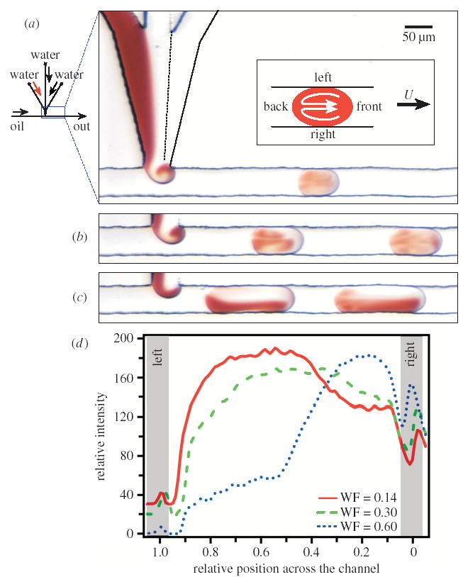
Formation of plugs from three aqueous solutions in a flow of immiscible fluorinated fluid in a microfluidic channel. Images also show the effects of the initial conditions of plug formation on the mixing of plugs moving through straight channels. (a)–(c) Left: a schematic of the microfluidic network. Right: microphotographs of plugs formed at water fractions of (a) 0.14, (b) 0.30 and (c) 0.60, respectively, from top to bottom. Plugs were travelling at 50 mm s⁻¹. The blue box indicates the region of the network shown. Red aqueous streams were solutions of 0.067 M [Fe(SCN)_x] ^(3−x)+ and colourless aqueous streams were 0.2 M KNO₃. The oil stream was a solution of water-immiscible fluorinated fluid (perfluorodecalin) with a (10:1) v/v ratio of 1H,1H,2H,2H-perfluoro-1-octanol. The inset in (a) is a schematic defining the sides of the plug relative to flow velocity U. (d) A graph of the relative optical intensity of red [Fe(SCN)_x] ^(3−x)+ complexes in plugs at WF = 0.14, 0.30 and 0.60 (lines). Grey shaded areas represent the walls of the microchannel on left (x = 1.0) and right (x = 0.0).

Dispersion is a problem associated with pressure-driven laminar flow in microfluidic channels (Bird et al. 2002). As the flow is parabolic, reagents move at different velocities across the width of the channel—slower along the walls but faster in the middle of the channel. Dispersion also occurs by the diffusion of reagents along the channel. Turbulence and mixing by chaotic advection may reduce dispersion, but localization of reagents in droplets removes it completely (Burns et al. 1998).

3. Mixing in plugs moving through straight channels

Recirculating flow is induced inside droplets moving through straight microfluidic channels. When a plug moves through a straight channel, two vortices are formed in the plug, one in the left half and the other in the right half of the plug (inset, figure 1a). This flow may be used to reduce the striation thickness and enhance mixing, as described by Handique & Burns (2001). For ideal initial conditions, the movement of a plug through a straight microchannel and the flows that result decrease the initial striation thickness from s_t(0) to s_t(d) by

$$s_{\text{t}}(d)=s_{\text{t}}(0)\times l/d,$$ (3.1)

where d (m) is the distance travelled by the droplet, and l (m) is the length of the droplet (Handique & Burns 2001).

We have shown (Tice et al. 2003) that the effectiveness of mixing inside a plug as it moves through a straight microchannel is sensitive to the initial distribution of the reagents in the plug, determined by the details of the plug’s formation. Ideally, in order to enhance mixing through the recirculating flow in the plug, the fluid must be distributed evenly throughout the left and right halves of the plug. In straight microchannels, an eddy forms as the aqueous phase is injected into the stream of carrier fluid, and this eddy distributes reagents to different regions of the plug. We refer to the formation of this eddy as ‘twirling’. We have shown that formation of the eddy is independent of flow velocity (Tice et al. 2003) and has been observed for the range of viscosities we work with (μ = 1–20 mPa s) and for a range of channel sizes (w = 20–200 μm). Ultimately, twirling depends on the relative volumetric flow rates of aqueous solutions and the carrier fluid, described by the ‘water fraction’. The water fraction is defined as WF = V_w/(V_w + V_f), where V_w and V_f are the volumetric flow rates of water, V_w (μl min⁻¹), and the fluorinated fluid, V_f (μl min⁻¹). If the WF of the flow is too low, then the eddy distributes reagents unevenly throughout the plug, as observed in figure 1a, as most of the red solution is distributed to the left half of the plug. This can be more clearly seen in the graph in figure 1d for WF = 0.14. This particular form of twirling is referred to as ‘over-twirling’. For a narrow range of values of WF, twirling distributes reagents evenly throughout the plug and enhances mixing (figure 1b). If the WF of the flow is high, the eddy does less to distribute reagents (figure 1c). Even under ideal conditions, the effectiveness of mixing inside a plug moving through a straight microchannel decreases as 1/d as the plug moves further through the channel (equation (3.1)) (Handique & Burns 2001; Ottino 1989).

4. Chaotic advection

Chaotic advection at low values of Re has been studied extensively in macroscopic flow cavities filled with viscous liquids (Ottino 1989). In a flow cavity, motion of the walls induces two-dimensional flow within the fluid, and we use it as a way to think about flows inside moving plugs. There are three differences between mixing inside a plug and mixing inside a flow cavity. First is a simple difference in the frame of reference: in the plug, the fluid moves relative to the stationary walls, but, in a flow cavity, the walls move relative to the fluid. The second difference is the direction of motion: in a plug, the fluid moves in the same direction relative to both walls. In a flow cavity, the walls can move independently in either direction relative to the fluid. The third difference is the dimensionality of the flow: inside a plug, the flow is three-dimensional, since the plug is in contact with both the side walls and the top/bottom walls. However, in the experiments described here, the solutes are distributed uniformly along the vertical dimension and mixing occurs primarily by the flow induced by side walls. Chaotic mixing in three-dimensional flows inside droplets is known to occur (Kroujiline & Stone 1999; Stone et al. 1991; Bryden & Brenner 1999).

When the motion of the walls in the flow cavity is steady, the fluid simply recirculates, as shown schematically in figure 2a(i). This recirculation induces rather inefficient mixing, as shown in figure 2a(ii) (Ottino et al. 1992; Ottino 1989). Such mixing is similar to mixing in a plug moving through a straight microchannel, with efficiency decreasing as 1/d, as discussed above. Due to the difference in the direction of motion of the fluid relative to the walls, there are two vortices induced inside a plug, as opposed to one vortex in a flow cavity (figure 2a(iii)). These two vortices mix the contents of each half of the plug, but there is no fluid exchange between the two halves, resulting in poor mixing.

Figure 2.

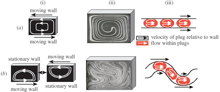
Comparing mixing in flow cavities and in plugs moving through microchannels. Mixing by (a) steady, recirculating flow and (b) chaotic advection. (i) Mixing represented by schemes of flow in a flow cavity; (ii) images of flow in a flow cavity (reproduced with permission of Cambridge University Press from Ottino (1989)); and (iii) schemes of flow in plugs moving through (a) a straight and (b) a winding channel.

When the motion of the walls in the flow cavity is unsteady (time-periodic) (figure 2b(i)), rapid mixing by chaotic advection is observed (figure 2b(ii)). Chaos cannot be generated in steady two-dimensional flows. In unsteady flows time becomes the third dimension, crossing of streamlines becomes possible, and chaos is induced (Ottino et al. 1992; Ottino 1989). Unsteady fluid flow resembling that in flow cavities is induced inside plugs moving through winding microchannels (figure 2b(iii)). The image in figure 2b(ii) shows chaotic mixing in a flow cavity with co-rotating vortices, although chaos can be generated in two counter-rotating vortices as well (Solomon & Gollub 1988; Jana et al. 1994). The flow in plugs moving through winding channels can be thought of in terms of two counter-rotating vortices (figure 2b(iii)) on the left and the right sides of the plug (defined in figure 2c), and plugs in winding channels chaotic advection has been shown to mix fluids rapidly (figure 3c) (Song et al. 2003b).

Figure 3.

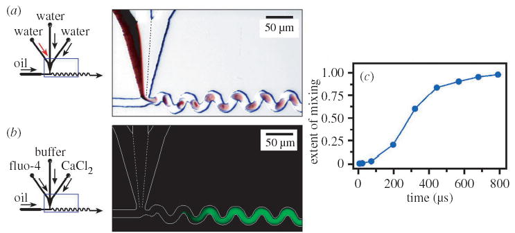
Inducing mixing by chaotic advection in plugs moving through microfluidic channels and quantifying this mixing by measuring fluorescence. (a) Left: schematic of the microfluidic network. Right: microphotograph (10 μs exposure) illustrating mixing. The solutions used were as in figure 1. (b) Left: schematic of the microfluidic network. Right: false-colour fluorescence microphotograph (2 s exposure, shows time-averaged intensity where individual plugs are not visible). The white lines trace the walls of the microchannel. The dashed white lines indicate the laminar flow of reagents in the junction of the aqueous inlet channels. Aqueous streams were solutions of 54 μM fluo-4, 70 μM CaCl₂ (both in 20 mM sodium morpholine propanesulfonate buffer (MOPS), pH 7.2) and 20 mM buffer. The oil stream was as in figure 1a. (c) A mixing profile obtained by analysing fluorescent images from a microchannel with smaller cross-sectional dimensions 10 μm × 10 μm.

5. Quantifying mixing

(a) The time–distance relationship

The mixing time of the reagents within the plug is related to the distance the plug has travelled in the channel. When the plug is travelling at a constant velocity, the distance the plug has moved through the channel since its formation is equivalent to the time the fluid isolated in the plug has mixed, as t = d/U, where t (s) is time, d (m) is distance travelled along the channel, and U (m s⁻¹) is the constant flow velocity. There is a thin film of carrier fluid that separates the plug from the walls of the microchannel (Bico & Qúeàe 2002), and there may be some slip between the two phases. However, our measurements of plug size under conditions used in this paper yield volume fractions virtually equivalent to expected values (Tice et al. 2003), which suggests that effects of slip are negligible. Therefore, this time–distance relationship is valid and can be used to perform and interpret kinetic measurements.

(b) Using fluorescence to quantify mixing

Fluorescence was used to quantify the mixing time through the time–distance relationship. We quantified mixing by measuring the intensity of the fluorescence generated by the binding reaction between Ca²⁺ and fluo-4 at different points along the channel, and therefore at different times in the progression of mixing (figure 3b). A mixing profile can be obtained by plotting measured intensity versus time (figure 3c). As the reaction is diffusion controlled, the time of the reaction corresponds to the mixing time. In the original microchannels (28 μm × 45 μm, figure 3b), mixing times of 1–2 ms were measured. Reducing the cross-sectional dimensions to 10 μm × 10 μm (Song et al. 2003b), among other improvements, moved mixing into the sub-millisecond regime (figure 3c). Scaling of mixing as a function of experimental conditions is described later in § 8.

(c) Challenges encountered when quantifying mixing

We have encountered two challenges when quantifying mixing. First, over-twirling and incomplete snap-off at the plug-forming region causes the time–distance relationship to break down. Mixed solution twirls up into the aqueous inlet of the plug-forming region (over-twirling) and a portion of it can be left there after the plug snaps off (incomplete snap-off) (figure 4a). Incomplete snap-off is illustrated further by the fluorescing spot at the inlet of the plug-forming region in the fluorescence image (figure 4b). These phenomena cause the solutions to mix for a longer time than predicted by the position of the plug in the channel—in fact, it is possible to create conditions under which plugs are completely mixed before snap-off—providing an apparent and incorrect mixing time of zero. Since the time of mixing of the solution at the inlet junction is not well defined under these conditions, quantifying the beginning of mixing is not possible.

Figure 4.

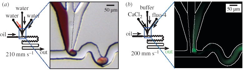
Over-twirling causes some mixed aqueous solutions to be left behind in the aqueous inlet of the plug-forming region after the plug snaps off, resulting in a poorly defined mixing time. (a) Left: schematic of the microfluidic network. Right: microphotograph of the plug-forming region of the microfluidic network. The aqueous streams were as in figure 1. The oil stream was as in figure 3a. The aqueous solution plug forming at the junction is uniform in colour, indicating that there is mixing at the junction. Mixed aqueous solution remains at the junction after the detachment of the plug. (b) Left: schematic of the microfluidic network. Right: false-colour fluorescence microphotograph (0.9 s exposure). The white lines trace the walls of the microchannel. Aqueous streams were solutions of 55.7 μM fluo-4, 150 μM CaCl₂ (both in 20 mM MOPS, pH 7.2) and 20 mM MOPS. The intense green spot at the aqueous inlet of the plug-forming region reveals that some mixed solutions remains there after each plug snaps off.

Second, it would be advantageous to increase the time-averaged fluorescence signal arising from the fluorescent plugs and non-fluorescent carrier fluid. In order to optimize mixing, plugs must be small but still touch all walls of the channel in order to create the recirculating flow in the fluid volume. These small plugs mix more effectively than larger plugs, as the efficiency of mixing depends on d/l, where d (m) is the distance the plug has moved through the channel and l (m) is the length of the plug. To do so with the geometry shown in figure 3, the water fraction must be small. At extremely low values of WF, the spatial period of the flow, or the centre-to-centre distance between adjacent plugs, increases. Consequently, at low values of WF, flow is characterized by small plugs separated by a length of oil around 4–5 times the plug length (Tice et al. 2003), leading to a lower density of plugs in the microchannel. This decreases the fluorescence signal, which is already limited by the short optical path, determined by the channel thickness (ca. 10–100 μm). A high density of small plugs travelling through the channel is desired.

(d) Overcoming the challenges of obtaining fluorescence intensity data

To solve the problems of quantifying and analysing fluorescence data, the channels in the plug-forming region were narrowed to half the width of the channels in the rest of the network (figure 5). The narrowed junction moves the point of snap-off further downstream. As seen in time-lapse images (figure 5a), the flow of aqueous solutions and the water-immiscible fluorinated fluid remains laminar through the narrowed region until the plug is formed (figure 5b). Presumably, the carrier fluid is flowing above and below the aqueous streams. In the plug that is formed, the red solution is completely isolated from the clear solution, indicating that there has been no twirling prior to formation of the plug, and no mixed solution has been left at the inlet. Because of the change in the region of snap-off, smaller plugs are formed, which also affects mixing (as discussed in § 6 below). This change is beneficial as the fluorescence signal increases because the new junction allows for the formation of smaller plugs that are much closer together than those formed in the wider inlet. The narrowed inlet preserves the time–distance relationship while providing an adequate fluorescent signal.

Figure 5.

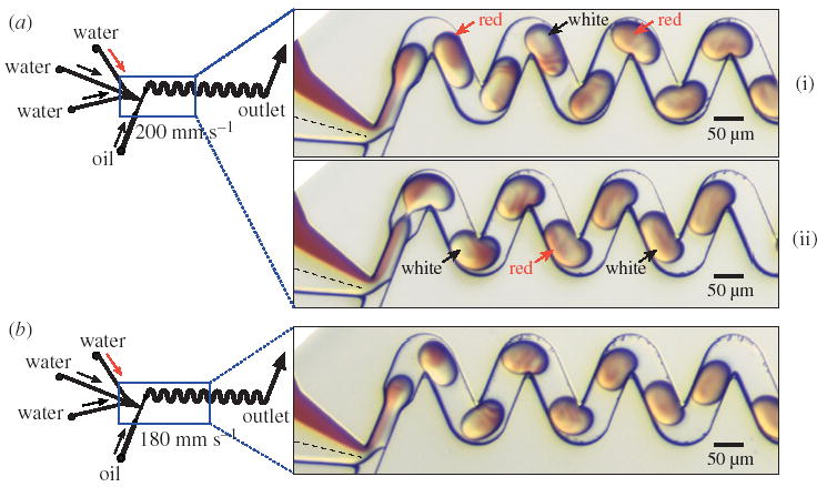
Chaotic advection in plugs moving through winding channels of various geometries. The narrowed channels at the plug-forming junction cause the aqueous solution to remain as distinct laminar streams until the formation of the plug. Left: schematic of the microfluidic network. Right: microphotographs of the microfluidic network. (a) Mixing in larger plugs (WF = 0.55). Arrows indicate ‘flipping’ of coloured solution in the back of the plug from one side to another. (b) Mixing in smaller plugs (WF = 0.44) is more efficient. In the smaller plugs, ‘flipping’ is not observed. The aqueous streams were as in figure 1. The oil stream was as in figure 3a.

6. Effects of channel geometry on chaotic mixing

Chaotic advection does not require a very specific geometry of winding channels. We have observed mixing by chaotic advection in a variety of winding microchannel geometries. Previously, we have used smooth turns to induce chaotic advection (Song et al. 2003b). We have also been able to generate chaotic advection in winding microchannels with sharp turns of 90° and 135°.

The size of the plugs (controlled by the WF, figure 1) formed in the channels affects the flow patterns observed inside the plugs, and affects mixing. Larger plugs, shown in figure 5a, form striations in the front of the plug, yet the back half of the plug appears to ‘flip’ the colours of its left and right sides (defined in figure 1a, inset), shown schematically by arrows in figure 5a. This flipping is a clear indication that mixing is not efficient throughout the plug. In chaotic advection, regions of poorly mixed solutions can exist even in the presence of chaos, and may be eliminated by randomizing the flows (Ottino et al. 1992). In the smaller plugs moving through the same channels (figure 5b), the striations form in the middle of the plug, ‘flipping’ is not observed, and mixing appears to be more efficient. Empirically, we have observed that mixing is best for plugs of a length approximately equal to two widths of the channel. In order to predict the geometry of microchannels that induces the most efficient mixing for each size of plugs, it is desirable to model the flow inside the plugs.

7. The baker’s transformation

In order to model mixing by chaotic advection inside plugs, we have used the baker’s transformation (Ottino & Wiggins 2004; Wiggins & Ottino 2004) as a guide. In the baker’s transformation, striation thickness decreases through a series of stretching, folding, and reorienting events as shown schematically at the top of figure 6. Mixing is very efficient because the striation thickness decreases exponentially according to

Figure 6.

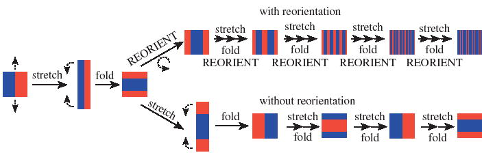
Schematic of a fluid element undergoing stretching, folding and reorientation, characteristics of the baker’s transformation (top). Stretching and folding, as defined here, without reorientation (bottom) does not lead to decrease of the striation thickness, demonstrating the critical nature of the reorientation step.

$$s_{\text{t}}(n)=s_{\text{t}}(0)\times 2^{-n},$$ (7.1)

where n is the number of fold, stretch and reorient cycles, s_t(0) is the initial striation thickness, and s_t(n) is the striation thickness after n cycles. For simplicity, we assumed that the Lyapunov exponent s = 2. This mixing by exponential decrease in striation thickness is similar to the ‘rolling droplet’ idea described by Fowler et al. (2002).

The baker’s transformation (figure 7a) is certainly an idealization of the mixing in plugs, but flow patterns reminiscent of the baker’s transformation can be observed experimentally inside plugs moving through microchannels (figure 7c). During one cycle, the plug experiences recirculating flow in the straight portions, which accounts for the folding and stretching, and then the plug reorients as it continues around a turn (shown schematically in figure 7a). The striation thickness decreases by a factor of two for each cycle, and as the cycles are repeated the striation thickness decreases exponentially according to equation (7.1).

Figure 7.

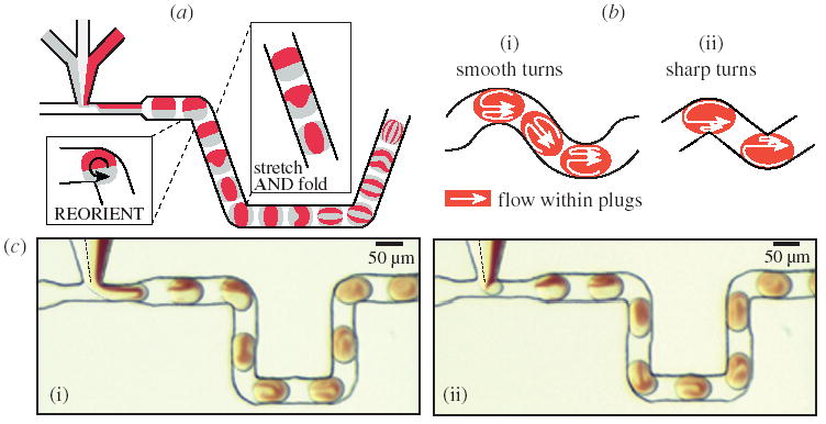
The baker’s transformation in plugs moving through a microfluidic channel. (a) Schematic illustrating the principle: straight portions of the channel perform stretching and folding, and turns allow for reorientation. (b) Mixing as represented by a scheme of recirculating flow in plugs moving through smooth turns (i) and sharp turns (ii). (c) Microphotographs of the microfluidic network in which flow patterns inside plugs in different positions in the microchannel demonstrate flow patterns reminiscent of the baker’s transformation. The aqueous streams were as in figure 1. The oil stream was 10:1 v/v perfluoro-1,3-dimethylcyclohexane to 1H,1H,2H,2H-perfluoro-1-octanol. The streams were flowed at 53 mm s⁻¹.

We emphasize that there is no fundamental difference in fluid flow within plugs moving through sharp turns or smooth turns present in winding channels. We believe that the effects of channel geometry on the recirculating flows can be seen by its effects on the two vortices within the plug. In a straight channel, these two vortices are symmetric (figure 2a(iii)). Around a smooth turn in a winding channel, the vortices are asymmetric (figure 7b(i)). Around a sharp turn, the asymmetry is large enough that the smaller vortex can be neglected and the flow within in the plug may be approximated by a single large vortex (figure 7b(ii)). This large vortex can be viewed as the reorientation of the whole plug in the baker’s transformation.

8. The scaling of mixing by chaotic advection

Chaotic mixing inside plugs moving through winding microchannels has been observed to obey a simple scaling argument that describes the dependence of mixing time on channel width, flow velocity and diffusion coefficient of reagents (Song et al. 2003a). The scaling argument was derived in the spirit of the baker’s transformation as has been done previously for chaotic mixing in general (Ottino 1994) and for chaotic mixing in microchannels (Stroock et al. 2002b). Two assumptions were made. First, we assumed that for one cycle of chaotic advection a plug must travel a distance equal to a certain number of its own lengths. To complete one cycle, the plug must travel the distance d(1) (m) that is proportional to the length of the plug, and in turn is proportional to the cross-sectional dimension of the microchannel: d(1) ~ l = a × w, where l (m) is the length of the plug, a is the length of the plug measured in widths of the channel, and w is the width of the microchannel. This assumption is justified and is convenient because the length of the plug is proportional to the channel width—as channels become smaller, plugs become smaller. For each cycle of chaotic advection the striation thickness decreases by a factor of s. Second, we assumed that the mixing time t_mix is approximately the time when the times for convective transport and diffusive mixing are matched. In other words, the mixing time is assumed to be approximately equal to the total residence time after which the diffusion time over the striation thickness is equal to or smaller than the already elapsed residence time.

From the first assumption, we estimated that the initial striation thickness is approximately equal to the width of the microchannel, s_t(0) ~ w, and that striation thickness for later positions is determined by the equation s_t(n) = w × σ⁻ⁿ. Inserting this definition of striation thickness into the equation for mixing purely by diffusion (equation (1.1)), the time-scale for mixing by diffusion after n cycles is

$$t_{\text{diff}}(n)=w^2\times {\sigma }^{-2n}/2D.$$ (8.1)

The time for transport by convection to complete n cycles was estimated to be

$$t_{\text{conv}}(n)\sim d(n)/U\sim n\times a\times w/U.$$ (8.2)

From the second assumption, we defined the mixing time t_mix to be when the time-scale for mixing by diffusion is equal to the time-scale for transport by convection (Stroock et al. 2002b):

$$t_{\text{conv}}(n)\sim n\times (a\times w/U)\sim w^2\times {\sigma }^{-2n}/2D=t_{\text{diff}}(n).$$ (8.3)

After rearrangement,

$$2a\times n\times {\sigma }^{2n}\sim w\times U/D=Pe,$$ (8.4)

where Pe is the Péclet number, defined as Pe = w × U/D.

The value of n is determined by taking the logarithm of both sides of equation (8.4) and assuming large values of the Péclet number:

$$n\sim log(Pe).$$ (8.5)

We assume large Pe when deriving the argument to be able to state that log(n) is much smaller than n × log(σ). By replacing the derived value of n in the equation for transport by convection, the mixing time t_mix,ca is defined:

$$t_{\text{mix},\text{ca}}\sim t_{\text{conv}}(n)\sim (a\times w/U)\times log(Pe).$$ (8.6)

The result that t_mix,ca ~ log(Pe) agrees with previous results for chaotic mixing (Ottino 1994), including mixing in structured microchannels (Stroock et al. 2002b).

In order to test the scaling argument, we performed a series of experiments (Song et al. 2003a) by independently varying flow velocity (U) by a factor of about 10, and the width of the channel (w) by a factor of 10. The diffusion coefficient was varied by a factor of about 10, and by quantifying mixing times using the Ca²⁺/fluo-4 binding (D ~ 1.6 × 10⁻⁹ m² s⁻¹) and cleavage of a fluorogenic substrate by RNase A (D ~ 2 × 10⁻¹⁰ m² s⁻¹) (Stellwagen & Stellwagen 2002). We used a random, general microchannel geometry shown in figure 8a. We plotted the intensity data from these experiments according to equation (8.6) (figure 8b). Mixing times were linearly related to (w/U) × log(Pe) as predicted by equation (8.6), in the range of parameters tested.

Figure 8.

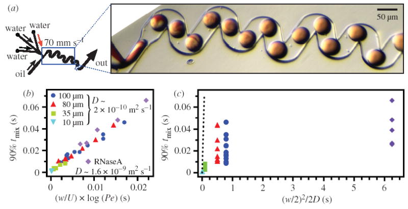
Experimental data showing scaling of mixing by chaotic advection. (a) Left: schematic of the design of the microfluidic network. Right: microphotograph of the plugs moving inside the channel used to determine the scaling of chaotic mixing. The aqueous streams were as in figure 1. The oil stream was as in figure 3a. (b) Mixing times t_mix data plotted as a function of (w/U) × log(Pe) as flow velocities U, cross-sectional dimensions of the microchannel w and the diffusion coefficient of the reagents D were varied. (c) Data from (b) replotted versus (w/2)²/2D, where s_t ~ (w/2). From these data, it is observed that chaotic mixing is much faster than mixing purely by diffusion (predicted mixing time purely by diffusion is shown by the dashed line with a slope of 1). For (b) and (c), 90% mixing time, 90% t_mix (s), was obtained from mixing profiles as in figure 3b.

The experimental value of t_mix for chaotic mixing differs greatly from the mixing time predicted for mixing purely by diffusion (the mixing times expected for mixing purely by diffusion are shown by the dashed line in figure 8c). A measure of the increase in effectiveness of chaotic mixing over diffusive mixing can be estimated by dividing the time of mixing by diffusion by the time of mixing through chaotic advection:

$$t_{\text{diff}}/t_{\text{mix}}=Pe/(a\times log(Pe)).$$ (8.7)

Chaotic advection mixes faster than diffusion alone by a factor of Pe/log(Pe), which has been shown previously for chaotic mixing (Ottino 1994). Chaotic advection increases the effectiveness of mixing the most for systems with high Péclet number, for example reagents with lower diffusion coefficients, and in flows with high flow rates inside large channels. It will not be as useful for accelerating mixing in systems where striation thickness is already small (e.g. in hydrodynamic focusing), but may offer complementary advantages in systems where slower, but complete mixing of multiple reagents in known ratios is required.

9. Using the microfluidic platform to measure kinetics

This plug-based microfluidic network can be used to perform kinetic measurements (Song & Ismagilov 2003). The system requires small amounts of reagents in order to perform experiments because rapid mixing is induced at low values of Re without resorting to turbulence, at flow rates of 10–100 nl s⁻¹. Rapid mixing and transport with no dispersion allows for accurate measurement of both fast and slow kinetic reactions. Rapid on-chip dilution in this system allows one to change the concentration of the reagents by simply varying the relative flow rates of the stock solutions, rather than replacing the stock solutions.

Understanding mixing quantitatively allowed us to incorporate mixing explicitly in the form of a mixing function f_m(t) into the kinetic model, so that kinetic parameters can be extracted from the data with resolution higher than that limited by the mixing time. As an example, we use a generic kinetic model for an enzymatic reaction [P] = F (k, [E]_o, [S], t), where [P] is the concentration of the product expressed in terms of time t, the rate constant k, the initial concentration of the enzyme [E]_o, and the concentration of the substrate [S]. The main effect of mixing occurring over a period of time t_mix is to spread the beginning of the reaction over a period of time t_mix. This effect can be analysed by separating the t_mix into small time-intervals. During a small time-interval dτ_i = τ_i+1 − τ_i, a fraction of the reaction mixture Δ f_m(τ_i) = f_m(τ_i+1) − f_m(τ_i) is mixed and begins to react with a time delay of τ. This effect may be incorporated into the kinetic expression

$$[P(t)]={\int }_0^{\infty }{f^{\prime }}_m(\tau )F(k,[S],t-\tau )\hspace{0.17em}\text{d}\tau .$$ (9.1)

This equation holds for simple kinetic models, but will not be correct for complex kinetic models, especially those modelling autocatalytic reactions (Metcalfe & Ottino 1994).

The form of the mixing function used to describe mixing is not important in this approach, as long as the derivative of the function can be found, and the function reproduces an experimentally determined mixing curve, such as one shown in figure 3c. The ability to establish the mixing function experimentally is an attractive feature of this system. We modelled mixing by a sigmoidal mixing function f_m(t),

$$f_{\text{m}}(t)=1/(1+\alpha exp(-\beta (t-\gamma ))),$$ (9.2)

where the dimensionless parameter a corresponds to the extent of asymmetry of the mixing curve, the parameter β (s⁻¹) describes the sharpness of the mixing curve, and the parameter γ(s) corresponds to the averaged mixing time. For this mixing function, f_m(t = 0) = 0 and f_m(t ≫ t_mix) = 1. The parameters were determined by fitting an experimentally determined mixing curve that was rescaled (using equation (8.6)) to the difference in diffusion coefficients between the components of the fluo-4/Ca²⁺ system used to measure mixing, and the components of the reaction for which kinetics was being measured.

Using this combined model of mixing and kinetics, we are able to describe the millisecond single-turnover kinetics of RNase A at pH = 7.5. For single-turnover kinetics, the initial concentration of the enzyme greatly exceeds that of the substrate, and the reaction can be described by the reaction equation:

$$[P(t)]={[S]}_{\text{o}}(1-exp(-kt)).$$ (9.3)

Using the fluo-4/Ca²⁺ system and then rescaling for the diffusion coefficient of the enzyme, we obtained the mixing function shown in figure 9. This mixing function was then incorporated into the kinetic model of the RNase A reaction:

Figure 9.

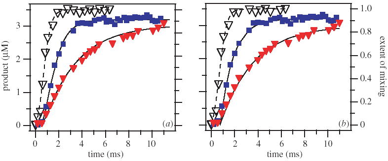
Using chaotic advection to measure millisecond single-turnover kinetics of RNase A at a pH of 7.5 and a pH of 6.0. The mixing function, determined experimentally by the fluo-4/Ca²⁺ system and then rescaled, is represented by the open triangles and fit with a sigmoidal curve (the dashed lines). (a) A graph of the experimental data (solid symbols) with fit produced by equation (9.4) of the reaction progress (solid lines) for both pH 7.5 (blue solid squares) and pH 6.0 (red solid triangles). (b) A graph of the experimental data (solid symbols) with the simple fits produced by equation (9.6) of the reaction progress (solid lines) for both values of pH.

$$[P(t)]={[S]}_{\text{o}}{\int }_0^{\infty }{f^{\prime }}_{\text{m}}(\tau )(1-exp(-k(t-\tau )))\hspace{0.17em}\text{d}\tau .$$ (9.4)

Equation (9.4) was used to fit the experimental data shown in figure 9a to give good fits with the rate constant of k = 1100 ± 250 s⁻¹, in agreement with the previously reported value (Thompson & Raines 1994). It is remarkable that such a fast rate constant (the half-life of the reaction mixture is only 0.6 ms) can be measured accurately and with high resolution in a system where mixing occurs on the same time-scale as the reaction. To verify that the agreement between the kinetic measurement performed on the microfluidic chip and the one previously reported is not coincidental, we repeated the measurement at pH = 6.0. Using the same mixing function, the rate constant of k = 350 ± 50 s⁻¹ was obtained from the fit, in agreement with the published pH dependence data for this reaction (Witzel 1963).

The fact that mixing occurs by chaotic advection is important for carrying out these high-resolution kinetic measurements. A simple argument can be used to demonstrate that the sharpness of mixing, rather than the total mixing time, is the most important parameter that determines the resolution with which kinetic parameters can be extracted from the data. The sigmoidal shape of a chaotic mixing curve ensures that even though mixing begins at time t = 0 and continues until t_mix, the majority of mixing occurs over a time-interval Δτ, where Δτ < t_mix. As mixing occurs over a shorter Δτ, the curve of the mixing function becomes steeper and steeper (or ‘sharper’). At its limit, the mixing function f_m(t) becomes Heaviside’s step function θ(t − t_mix). The derivative of this stepwise function is equal to Dirac’s delta function (θ(t − t_mix)′ = δ(t − t_mix)). Rewriting equation (9.1) gives

$$[P(t)]={\int }_0^{\infty }\delta (\tau -t_{\text{mix}})F(k,[S],t-\tau )\hspace{0.17em}\text{d}\tau .$$ (9.5)

As δ(τ − t_mix) is equal to zero everywhere except at t_mix, the kinetic model simplifies to

$$[P(t)]=F(k,[S],t-t_{mi\text{x}}).$$ (9.6)

When mixing becomes infinitely sharp at time t_mix, the kinetic model for the reaction simplifies to the original kinetic model in which the time variable is shifted by the term t_mix.

Chaotic advection is attractive in this respect because mixing is sharp. The 90% mixing time is ca. 1.5 ms, but over 50% of the solution is mixed in only 0.4 ms, from t = 0.4 ms to t = 0.8 ms. We have illustrated this fact by using the approximate equation (9.6) to fit the experimental data using a time delay of 0.75 ms (experimentally determined average mixing time is 0.72 ms) (figure 9b). We obtained adequate fits for pH = 7.5 with the rate constant k = 1000 ± 300 s⁻¹, similar to that obtained from equation (9.4) using explicit treatment of mixing. Slower reaction at pH = 6.0 gave a good fit with the rate constant k = 350 ± 50 s⁻¹, using the same time delay of 0.75 ms. This argument suggests a somewhat counterintuitive point. Pre-mixing (mixing before snap-off) of solutions—for example, mixing that occurs in the process of twirling during the formation of the plugs—may slightly reduce total mixing time. However, it is detrimental for high-resolution kinetic measurements when mixing is performed by chaotic advection. It is likely to significantly broaden the mixing curve, leading to a wide distribution of mixing times and less-resolved kinetic measurements.

10. Conclusion

In this work, we have learned that chaotic advection can be induced in plugs moving through a variety of winding geometries as long as time-periodic flows are induced. Winding channels created chaotic mixing by folding, stretching and reorienting the fluid volume. Using a random, winding microchannel geometry, we have quantified the scaling of chaotic mixing over at least a 10-fold range of channel widths, flow velocities and diffusion coefficients, making it useful for a wide range of experiments. We found that mixing by chaotic advection accelerated mixing most for systems with a high Péclet number. This method of mixing did not rely on turbulence, and required a small volume of sample; absence of dispersion further minimized the sample consumption, making this system attractive for performing kinetic experiments with biological and other samples available in small quantities. Simple mathematical treatment was developed that incorporated mixing into kinetic models that extract kinetic parameters with high resolution. The development of this system has been driven by understanding the fascinating phenomena that occur in these multiphase fluid flows inside microchannels. Deeper understanding, e.g. detailed predictive modelling of the flows inside moving plugs, is certain to improve this system further.

References

- Ali JA, Lohman TM. Kinetic measurement of the step size of DNA unwinding by Escherichia coli UvrD helicase. Science. 1997;275:377. doi: 10.1126/science.275.5298.377. [DOI] [PubMed] [Google Scholar]
- Aref H. Stirring by chaotic advection. J Fluid Mech. 1984;143:1. [Google Scholar]
- Bico J, Quéré D. Self-propelling slugs. J Fluid Mech. 2002;467:101. [Google Scholar]
- Bird RB, Stewart WE, Lightfoot EN. Transport phenomena. Wiley; 2002. [Google Scholar]
- Brazeau BJ, Austin RN, Tarr C, Groves JT, Lipscomb JD. Intermediate Q from soluble methane monooxygenase hydroxylates the mechanistic substrate probe norcarane: evidence for a stepwise reaction. J Am Chem Soc. 2001;123:11831. doi: 10.1021/ja016376+. [DOI] [PubMed] [Google Scholar]
- Bryden MD, Brenner H. Mass-transfer enhancement via chaotic laminar flow within a droplet. J Fluid Mech. 1999;379:319. [Google Scholar]
- Burns MA. An integrated nanoliter DNA analysis device. Science. 1998;282:484. doi: 10.1126/science.282.5388.484. (and 11 others) [DOI] [PubMed] [Google Scholar]
- Duffy DC, McDonald JC, Schueller OJA, Whitesides GM. Rapid prototyping of microfluidic systems in poly(dimethylsiloxane) Analyt Chem. 1998;70:4974. doi: 10.1021/ac980656z. [DOI] [PubMed] [Google Scholar]
- Fowler J, Moon H, Kim CJ. Proc 2002 IEEE 15th Int Conf Micro Electro Mechanical Systems; Las Vegas, NV. Piscataway, NJ: IEEE; 2002. [Google Scholar]
- Handique K, Burns MA. Mathematical modeling of drop mixing in a slit-type microchannel. J Micromech Microengng. 2001;11:548. [Google Scholar]
- Jana SC, Metcalfe G, Ottino JM. Experimental and computational studies of mixing in complex Stokes flows—the vortex mixing flow and multicellular cavity flows. J Fluid Mech. 1994;269:199. [Google Scholar]
- Kakuta M, Jayawickrama DA, Wolters AM, Manz A, Sweedler JV. Micromixer-based time-resolved NMR: applications to ubiquitin protein conformation. Analyt Chem. 2003;75:956. doi: 10.1021/ac026076q. [DOI] [PubMed] [Google Scholar]
- Kerby M, Chien RL. A fluorogenic assay using pressure-driven flow on a microchip. Electrophoresis. 2001;22:3916. doi: 10.1002/1522-2683(200110)22:18<3916::AID-ELPS3916>3.0.CO;2-V. [DOI] [PubMed] [Google Scholar]
- Knight JB, Vishwanath A, Brody JP, Austin RH. Hydrodynamic focusing on a silicon chip: mixing nanoliters in microseconds. Phys Rev Lett. 1998;80:3863. [Google Scholar]
- Krantz BA, Sosnick TR. Distinguishing between two-state and three-state models for ubiquitin folding. Biochemistry. 2000;39:11 696. doi: 10.1021/bi000792+. [DOI] [PubMed] [Google Scholar]
- Kroujiline D, Stone HA. Chaotic streamlines in steady bounded three-dimensional Stokes flows. Physica D. 1999;130:105. [Google Scholar]
- Liu RH, Stremler MA, Sharp KV, Olsen MG, Santiago JG, Adrian RJ, Aref H, Beebe DJ. Passive mixing in a three-dimensional serpentine microchannel. J Microelectromech Syst. 2000;9:190. [Google Scholar]
- McDonald JC, Whitesides GM. Poly(dimethylsiloxane) as a material for fabricating microfluidic devices. Acc Chem Res. 2002;35:491. doi: 10.1021/ar010110q. [DOI] [PubMed] [Google Scholar]
- McDonald JC, Duffy DC, Anderson JR, Chiu DT, Wu HK, Schueller OJA, Whitesides GM. Fabrication of microfluidic systems in poly(dimethylsiloxane) Electrophoresis. 2000;21:27. doi: 10.1002/(SICI)1522-2683(20000101)21:1<27::AID-ELPS27>3.0.CO;2-C. [DOI] [PubMed] [Google Scholar]
- Mao HB, Yang TL, Cremer PS. Design and characterization of immobilized enzymes in microfluidic systems. Analyt Chem. 2002;74:379. doi: 10.1021/ac010822u. [DOI] [PubMed] [Google Scholar]
- Metcalfe G, Ottino JM. Autocatalytic processes in mixing flows. Phys Rev Lett. 1994;72:2875. doi: 10.1103/PhysRevLett.72.2875. [DOI] [PubMed] [Google Scholar]
- Ottino JM. The kinematics of mixing: stretching, chaos, and transport. Cambridge University Press; 1989. [Google Scholar]
- Ottino JM. Mixing and chemical-reactions—a tutorial. Chem Engng Sci. 1994;49:4005. [Google Scholar]
- Ottino JM, Wiggins S. Introduction. Phil Trans R Soc Lond A. 2004;362:923–935. doi: 10.1098/rsta.2003.1355. [DOI] [PubMed] [Google Scholar]
- Ottino JM, Muzzio FJ, Tjahjadi M, Franjione JG, Jana SC, Kusch HA. Chaos, symmetry, and self-similarity—exploiting order and disorder in mixing processes. Science. 1992;257:754. doi: 10.1126/science.257.5071.754. [DOI] [PubMed] [Google Scholar]
- Pollack L. Time resolved collapse of a folding protein observed with small angle X-ray scattering. Phys Rev Lett. 2001;86:4962. doi: 10.1103/PhysRevLett.86.4962. (and 10 others) [DOI] [PubMed] [Google Scholar]
- Russell R. Rapid compaction during RNA folding. Proc Natl Acad Sci USA. 2002;99:4266. doi: 10.1073/pnas.072589599. (and 10 others) [DOI] [PMC free article] [PubMed] [Google Scholar]
- Shastry MCR, Luck SD, Roder H. A continuous-flow capillary mixing method to monitor reactions on the microsecond time scale. Biophys J. 1998;74:2714. doi: 10.1016/S0006-3495(98)77977-9. [DOI] [PMC free article] [PubMed] [Google Scholar]
- Solomon TH, Gollub JP. Chaotic particle-transport in time-dependent Rayleigh–Bénard convection. Phys Rev A. 1988;38:6280. doi: 10.1103/physreva.38.6280. [DOI] [PubMed] [Google Scholar]
- Song H, Ismagilov RF. Millisecond kinetics on a microfluidic chip using nanoliters of reagents. J Am Chem Soc. 2003;125:14613. doi: 10.1021/ja0354566. [DOI] [PMC free article] [PubMed] [Google Scholar]
- Song H, Bringer MR, Tice JD, Gerdts CJ, Ismagilov RF. Scaling of mixing by chaotic advection in droplets moving through microfluidic channels. Appl Phys Lett. 2003a;83:4664. doi: 10.1063/1.1630378. [DOI] [PMC free article] [PubMed] [Google Scholar]
- Song H, Tice JD, Ismagilov RF. A microfluidic system for controlling reaction networks in time. Angew Chem Int Ed. 2003b;42:768. doi: 10.1002/anie.200390203. [DOI] [PubMed] [Google Scholar]
- Stellwagen E, Stellwagen NC. Determining the electrophoretic mobility and translational diffusion coefficients of DNA molecules in free solution. Electrophoresis. 2002;23:2794. doi: 10.1002/1522-2683(200208)23:16<2794::AID-ELPS2794>3.0.CO;2-Y. [DOI] [PubMed] [Google Scholar]
- Stone HA, Nadim A, Strogatz SH. Chaotic streamlines inside drops immersed in steady Stokes flows. J Fluid Mech. 1991;232:629. [Google Scholar]
- Stroock AD, Dertinger SK, Whitesides GM, Ajdari A. Patterning flows using grooved surfaces. Analyt Chem. 2002a;74:5306. doi: 10.1021/ac0257389. [DOI] [PubMed] [Google Scholar]
- Stroock AD, Dertinger SKW, Ajdari A, Mezic I, Stone HA, Whitesides GM. Chaotic mixer for microchannels. Science. 2002b;295:647. doi: 10.1126/science.1066238. [DOI] [PubMed] [Google Scholar]
- Thompson JE, Raines RT. Value of general acid-base catalysis to ribonuclease-A. J Am Chem Soc. 1994;116:5467. doi: 10.1021/ja00091a060. [DOI] [PMC free article] [PubMed] [Google Scholar]
- Tice JD, Song H, Lyon AD, Ismagilov RF. Formation of droplets and mixing in multiphase microfluidics at low values of the Reynolds and capillary numbers. Langmuir. 2003;19:9127. [Google Scholar]
- Wiggins S, Ottino JM. Foundations of chaotic mixing. Phil Trans R Soc Lond A. 2004;362:937–970. doi: 10.1098/rsta.2003.1356. [DOI] [PubMed] [Google Scholar]
- Witzel H. The function of the pyrimidine base in the ribonuclease reaction. Prog Nucleic Acid Res Mol Biol. 1963;2:221. [Google Scholar]
- Zheng B, Roach LS, Ismagilov RF. Screening of protein crystallization conditions on a microfluidic chip using nanoliter-size droplets. J Am Chem Soc. 2003;125:11 170. doi: 10.1021/ja037166v. [DOI] [PubMed] [Google Scholar]