Contributions of Gaussian Curvature and Nonconstant Lipid Volume to Protein Deformation of Lipid Bilayers

Abstract

An elastic model for membrane deformations induced by integral membrane proteins is presented. An earlier theory is extended to account for nonvanishing saddle splay modulus within lipid monolayers and perturbations to lipid volume proximal to the protein. Analytical results are derived for the deformation profile surrounding a single cylindrical protein inclusion, which compare favorably to coarse-grained simulations over a range of protein sizes. Numerical results for multi-protein systems indicate that membrane-mediated interactions between inclusions are strongly affected by Gaussian curvature and display nonpairwise additivity. Implications for the aggregation of proteins are discussed.

INTRODUCTION

Transmembrane proteins perform critical biological roles as receptors, enzymes, channels, and structural elements within cells (1). Acting as the environment surrounding these proteins, the membrane can influence protein function. Although some of this influence is likely due to specific and detailed lipid-protein interactions, experiments point to the elastic properties of the membrane as playing a prominent role in the activity of certain proteins. For example, both gramicidin A channels (2,3) and bacteriorhodopsin (4) seem critically dependent on the thickness of the surrounding bilayer and associated elastic properties for proper biological behavior. Fully understanding the behavior of membrane proteins, both as individual units and as larger complexes, requires a detailed understanding of lipid-bilayer biophysics from both molecular and continuum (elastic) perspectives. This article focuses on elastic properties with confirmation via coarse-grained molecular level simulations.

When two components of a membrane naturally span hydrophobic regions of different size, they are said to be “hydrophobically mismatched”. If the hydrophobic region of a specific molecule (such as a protein) is shorter than the average thickness of the surrounding membrane, the molecule is “negatively mismatched”; the reverse scenario is called “positive mismatch” (Fig. 1). The large interfacial tension between water and hydrophobic structures drives the membrane to deform so as to shield hydrophobic regions from water, as in Fig. 1. The resulting shape or “deformation profile” of the bilayer around such an imposed disruption depends upon the details of the protein and the lipid environment. Hydrophobic mismatch and its implications have been studied from experimental (2,3,6,7), theoretical (6,8–18), and computational (18–23) perspectives.

FIGURE 1.

Inclusion induced deformation (positive mismatch case). A symmetric transmembrane protein with hydrophobic residues around its periphery exceeding the thickness of the surrounding membrane will tend to distort the bilayer as shown (not to scale). A protein thinner than the surrounding membrane (negative mismatch) is expected to induce the opposite effect. The nonmonotonic deformation profile in membrane thickness as one moves away from the inclusion is predicted theoretically by continuum elastic models and is observed in simulations.

Historically, continuum elastic theories for the mismatch problem, when tested, have been tested against experimental data; the results indicate the plausibility of elastic theories but are inconclusive with regard to distinguishing among the various models currently proposed. For instance, the models of Huang (8), Brannigan and Brown (18), and Nielsen (15) all predict gramicidin lifetime data in good agreement with experiment despite significant differences from one elastic model to the next. Given the somewhat indirect comparison between theory and experimental observables, this is not surprising. Recent advances in computational modeling have allowed simulation studies (18–23) of the hydrophobic mismatch problem with the potential for more critical analysis of elastic theories. Unfortunately, the focus of most of these studies has not been on testing analytical theory, so refinement of elastic models with input from simulation data has not yet occurred.

In a recent study, we presented an elastic theory described as “consistent” (18) in its correct description of thermal bilayer fluctuations and mismatch-type bilayer deformations as tested against available simulation data. To our knowledge, that study represents the first detailed comparison between elastic theory and simulations in the context of the hydrophobic mismatch problem. One implication of that study is that the elastic theory of Aranda-Espinoza et al. (13) (henceforth referred to as A-E) works very well, predicting deformation profiles around a cylindrical protein inclusion in quantitative agreement with simulation results without any fit parameters. (In the case of protein-induced deformations for most relevant parameter regimes, the theory we suggested in our earlier study reduces to that of A-E.) However, this finding needs to be presented with two qualifiers. First, our simulation test was restricted to a coarse-grained model. Second, and more relevant to the work presented here, we only directly verified the theory of A-E for a single size cylindrical inclusion at a positive mismatch.

This study began as a series of simulations paralleling the single inclusion study presented in our earlier work. Fourteen different cylindrical protein inclusions spanning both positive and negative mismatches and a range of radii were simulated. We found that the agreement between theory and experiment reported in our earlier work was fortuitous. Only at positive mismatch does the existing theory do a good job at predicting deformation profiles. To explain all 14 data sets, it is necessary to reconsider the elastic theory of A-E. The version of the theory presented herein includes the energetics associated with Gaussian curvature deformations and the fact that a protein inclusion has the ability to locally alter the average volume per lipid in its immediate vicinity. With these additions, we find universally good agreement between theory and simulation, indicating a broad region of applicability for the improved theory. The new additions have no effect on bilayer fluctuations in homogeneous systems, so we believe the theory presented here is now truly consistent in its proper description of both fluctuations and deformation profiles.

Energetics associated with Gaussian curvature are typically neglected in elastic treatments of the mismatch problem. Although a few studies have recognized the possible contribution of finite saddle splay modulus to deformation profiles (14,17,24), these studies have gone on to ultimately neglect these effects either through judicious choice of boundary conditions or by appealing to arguments that the contributions should be negligible for “typical” physical constants. In our earlier work (18), we argued for the use of natural boundary conditions (as in A-E), both due to mathematical elegance and simulation results in contradiction with other common schemes. Natural boundary conditions predict that the saddle splay modulus should (at least formally) enter into all final results. For the coarse-grained systems studied in this work (which display elastic moduli comparable to experimental lipid systems), we find the contributions of Gaussian curvature are essential to obtain uniform agreement with simulation over a range of inclusion sizes.

We are not aware of prior studies that explicitly consider nonconservation of lipid volume. A lipid in a fluid bilayer has a volume compressibility modulus close to that of water and much larger than the bilayer area compressibility modulus (25). Naively, one expects that the thickness deformations should be accompanied by fully compensating area deformations, resulting in a near constant volume per lipid. Although this reasoning holds true for a homogeneous bilayer, it is important to realize that the imposition of an effective boundary (the protein surface) can alter fluid structure in ways that are difficult to predict. Even in “simple” systems of Lennard-Jones fluids, an imposed boundary can introduce local density deviations that are a challenge to predict theoretically (26). In our theory, we take lipid volume deformation near the protein to be an imposed perturbation; i.e., we do not attempt to solve for the volume deformation profile. We extract the volume deformation profile directly from simulation and input the results in our theory. In most of our discussion, we further assume this deformation is completely confined to the interface between protein and bilayer—this leads to analytically tractable solutions, which display close agreement with simulations.

Under certain circumstances, thickness deformations caused by hydrophobic mismatch can be alleviated by protein aggregation. For instance, experimental distributions of bacteriorhodopsin indicate an attraction between proteins, and at sufficient mismatches (−10% and +20%) the proteins aggregate (4). Synthetic transmembrane peptides with smaller radii than bacteriorhodopsin also dimerize and trimerize at certain mismatches (5). The work presented here predicts membrane-mediated protein interactions with increased sensitivity to mismatch amplitude relative to the original model of A-E. The improved model accounts for qualitative features of these experiments lacking from previous models.

THEORY

An analytical model for membrane thickness deformations induced by cylindrical proteins is derived below. The theory directly builds on that presented in A-E, adding the possibility of variable volume per lipid and allowing for finite saddle splay modulus. The discussion presented here has, to the extent possible, been presented in a notation consistent with our earlier work (18). Our treatment is quite terse, with readers directed to A-E and our earlier work for more details.

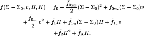
A single lipid in a flat homogenous bilayer assumes, on average, area Σ₀, thickness t₀, and volume v₀ = Σ₀t₀. All deviations are measured relative to this fiducial state. Deviations come in the form of local changes in the area/lipid (as measured perpendicular to the local monolayer normal), volume/lipid, and curvature of the monolayer surface. Membrane fluidity dictates that only invariants of the curvature tensor be included in the Hamiltonian (27,28); these include the trace (twice the mean curvature, H) and the determinant (the Gaussian curvature, K). Expanding to second order in all deviations (curvature, lipid volume, lipid area) from the reference state we find an expression for the free energy per molecule:

(1)

Here we have introduced a considerable amount of notation. Σ is the area per molecule, v + v₀ is the volume per molecule, and is the free energy per molecule (the quantity f being reserved for the free energy per unit area (18)). Note that whereas Σ is the true area per molecule, v is the deviation in volume per molecule from the reference state. Similarly, t is used to indicate deviations in monolayer (lipid) thickness relative to t₀. Coefficients in the Taylor expansion are named with the following convention adopted from Safran (27): derivatives of with respect to H are denoted with a numerical subscript indicating the order of differentiation. Derivatives with respect to other variables are denoted with the appropriate symbols. So, for example, . Note that since K is itself second order in curvature deformations, there are no cross derivatives with the Gaussian curvature or terms of second order in K. Our notation is slightly different from that used in our earlier work (18), due to the introduction of derivatives with respect to v and K.

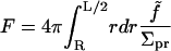
Assuming a vanishing lipid chemical potential (i.e., zero surface tension), it follows that and the free energy for the bilayer is given by summing the remaining terms of Eq. 1 over all lipids in the bilayer. In practice, this summation is conveniently carried out by integrating over the projected area of the bilayer sheet. We assume the inclusion has the symmetry indicated in Fig. 1 so that both monolayers share the same energy, their shapes superpose upon reflection through the xy plane, and the deformation is radially symmetric around the center of the inclusion. The elastic free energy for the bilayer associated with a given symmetric distortion is then

(2)

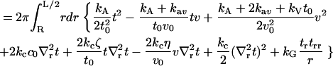(3)

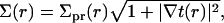
We have introduced a circular annulus for the integration region spanning the area between the inclusion radius, R and some maximal radius L/2. (This region is convenient for analytical work. In our numerical treatments, we use a square box and the integration region must be altered accordingly.) Σ_pr is the area per lipid projected onto the reference xy plane,

(4)

where t(r) + t₀ is the local thickness of the monolayer (see Fig. 1). In deriving Eq. 3 from Eq. 2, we have expressed all areas per molecule in terms of local monolayer thickness and volume per lipid. The following definitions were used in this step, which, although approximate, ensure a consistent final result up to second order in t(r) and v(r):

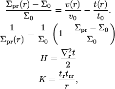(5)

where t_r ≡ ∂t/∂r, t_rr ≡ ∂²t/∂r², and 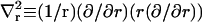. When possible, the constants in Eq. 3 were expressed using their common names: k_A is the bilayer area compressibility modulus, k_V is the bilayer volume compressibility modulus, c₀ is the spontaneous curvature of the monolayer, and are its area and volume derivatives respectively, evaluated at zero tension, k_c is the bilayer bending modulus, and k_G is twice the monolayer saddle splay modulus. The thickness-volume cross-term modulus has been assigned the name k_av. We have defined and .

Equation 3 expresses the elastic energy associated with a radially symmetric distortion of the bilayer with additional mirror symmetry through the xy plane. The free energy is a functional of two fields: the thickness deviations of the associated monolayers, t, and deviations in volume per lipid, v. Prior theories have neglected v entirely. Most prior theories have also assumed (explicitly or otherwise) k_G = 0. In the case that v = k_G = 0, Eq. 3 reduces to the free energy derived by A-E and the free energy considered in our earlier work (18) in the limit of uncoupled protrusion modes.

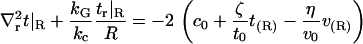
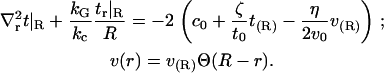
From this point forward, we assume the volume deformation field is a known function. In practice, we will extract v(r) directly from simulations as input to our theory. (Determining an appropriate equation of state for an inhomogeneous and anisotropic fluid near an imposed boundary seems a formidable problem, which we avoid by assuming v(r) is known.) Deformation shape is then determined by minimizing F over all possible t(r), which yields a solution in the form of a differential equation,

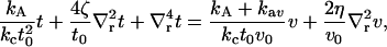(6)

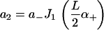
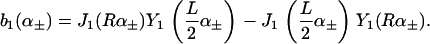
where . We note that neither k_G nor c₀ appear in the Euler-Lagrange equation. They do affect the overall solution through our choice of boundary conditions. The homogeneous equation (v = 0 case) has a solution of the form (13)

(7)

where J₀ and Y₀ are zeroth order Bessel functions of the first and second kinds, (29) respectively, α_± are the frequencies of oscillation, and a_n are coefficients determined by the boundary conditions. Below, we impose an additional restriction on v(r), making it possible to express the solution of Eq. 6 in terms of a solution to the homogeneous problem; the details of the solution used in this work are specified in the Appendix.

The choice of boundary conditions in the mismatch problem has been a subject of considerable controversy. Without further comment (see our earlier work (18) for discussion), we adopt the boundary conditions initially suggested by A-E. We set the membrane height equal to the inclusion height at the inclusion boundary, or

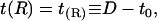(8)

where R is the radius of the inclusion and D is the inclusion half-thickness. At the far edge of the integration region we set the slope to zero:

(9)

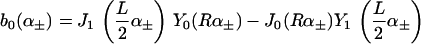
For the remaining two conditions, we adopt the so-called “natural” boundary conditions that are implied by the minimization of F if no further conditions are imposed. This results in one more condition at each edge of the region,

(10)

(11)

where v_(R) ≡ v(R) is the volume deformation at the lipid inclusion boundary, , and we have assumed that v_r|_L/2 = 0. Our analysis will primarily focus on deformation profiles of isolated proteins where L is taken large enough that t and v have completely relaxed at the outer edge of the considered region. Hence, our reported results are not sensitive to the exact choices in Eqs. 9 and 11. In their original work, A-E considered proteins in crystalline geometries up to the close packed limit and all conditions had impact on the final results. Below (“Free energy of multiple inclusions”), we do consider proteins in close proximity, but treat the situation numerically as a many protein problem (not as a single protein problem), so the issue of boundary conditions at the far edge never comes up. Of course, conditions 8 and 10 are relevant to all calculations and contain the sole influence of k_G and c₀ on the deformation profile.

One point should be indicated regarding the natural boundary condition (Eq. 10) at R. It appears that k_G should become less important as protein radius increases, simply due to the R⁻¹ dependence in the only term involving k_G. Physically, the limit corresponds to a flat, wall-like inclusion. In this limit, only one principal curvature of the surface is nonzero and the Gaussian curvature necessarily vanishes, leaving no possible influence for k_G. We therefore expect the influence of k_G on deformation profiles will be most pronounced when protein radius is small. This effect is clearly seen in our simulations below.

In principle, we could proceed directly from the equations presented. For a given inclusion, we would extract v(r) from simulation (or some other source) and use this function in Eq. 6, solving for the energy minimizing t(r) using the suggested boundary conditions. However, we lack a theory for and hence any analytical expression for use as v(r). Furthermore, simulations suggest that v(r) is a quickly decaying function (“Simulation results: volume deformation”). This suggests a simplifying approximation that we have verified numerically in several test cases. We treat the volume perturbation as being completely localized to the lipid-protein boundary. Mathematically, we take

(12)

With this form for v(r) and our specified boundary conditions, the full Eq. 6 is analytically solvable. The solution has the same form as Eq. 7, with the same frequencies as the homogeneous solution but with altered coefficients a_n. Since the modification to the homogeneous solution induced by Eq. 12 is found in the expansion coefficients alone, this change may equivalently be regarded as a change to the boundary conditions for the homogeneous problem. The corresponding change is physically transparent and amounts to averaging Eq. 10 over the jump in v present at the boundary. That is, we make the replacement to give

(13)

The factor of 1/2 accounts for the abrupt change in volume/lipid right at the boundary of the protein. In practical terms, η is not a known quantity and will be used as a fitting constant in the analysis presented below. All further analytical results assume the volume deformation profile of Eq. 12. Exact analytical solutions are reported in the Appendix, and were verified through numerical solution of Eq. 6 with boundary condition 10 using a smoothed version of the Heaviside function slightly displaced from r = R.

The minimized t(r) may be substituted back into Eq. 3 to obtain an expression for the energetic cost of protein insertion associated with bilayer elasticity. With our chosen form for v(r), the volume stretching terms in the Hamiltonian just integrate to constants (i.e., these terms are not dependent on t(r)). Neglecting these constants and using the boundary conditions (Eqs. 8–11) for simplification yields

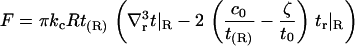(14)

We note that this expression is not unique in the sense that, for example, Eq. 10 can be used to recast c₀ in terms of other quantities. In particular, the expression could be rewritten to make the influence of k_g and η explicit. As presented, the influence of k_g and η on membrane energetics is implicitly contained within Eq. 14 through the shape of the membrane surface at contact. Equation 14 appears identical to the original (k_G = v = 0) results of A-E, but the implicit influence of k_g and η on this equation gives rise to deviations from the A-E results. In the section “Free energy of multiple inclusions”, we present numerical calculations to obtain the interaction energetics between multiple inclusions.

SIMULATIONS

Generation of data

We use the solvent free lipid model described in Brannigan et al. (30) for our simulations. The model has three building blocks: hydrophobic beads, hydrophilic beads, and interface beads. Hydrophobic beads attract each other through standard Lennard-Jones interactions and hydrophilic beads are purely repulsive. Interface beads are placed between the hydrophobic and hydrophilic beads; they interact through a soft potential that mimics oil-water interfacial tension. Individual lipids consist of one hydrophilic bead, one interface bead, and three hydrophobic beads linearly connected along a semiflexible backbone (Fig. 2); membranes formed by this model are fluid, self-assemble, and have elastic properties in the range of biological relevance. (31) Furthermore, they have stress profiles qualitatively similar to solvated bilayers simulated with atomistic resolution (32) and quantitatively similar to solvated bilayers simulated with a similar level of coarse graining (33). The stress profile is relevant when considering the behavior of inclusions embedded within the membrane, so this is an important correspondence. Our earlier work (18) extended this model to consider “proteins” embedded in a lipid bilayer. These proteins are constructed as a rigid assembly of the same hydrophobic, hydrophilic, and interface beads used for the lipids (Fig. 2). The energetic parameters defining lipid/protein beads are the same as those used in our earlier work (18).

FIGURE 2.

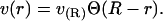
(Left) Range of inclusion structures used in this present study. Simulations are run for two different thickness mismatches (both shown), and seven different radii (smallest and largest shown) for a total of 14 simulations. A model lipid is also shown for comparison: the inclusion with four layers of hydrophobic beads (top) is mismatched primarily because it has fewer hydrophobic beads than a pair of lipids, whereas the inclusion with six layers of hydrophobic beads (bottom) is mismatched because it is rigid and the lipids are flexible. Hydrophobic beads are white, interface beads are gray, and hydrophilic beads are black. (Right) Inclusions (gray) of radius R = 3 nm embedded in membrane (cross section). The pinching of the membrane caused by negative hydrophobic mismatch (top) and dilation caused by positive mismatch (bottom) are visible.

The study presented here repeats the numerical experiment of our earlier work, but with many different sizes of the protein inclusions (Fig. 2). Inclusion radius R is varied through the number of concentric rings of beads comprising the cylinder. The inclusion half-thickness D is varied through the number of layers of hydrophobic beads. Inclusions with seven values of R ranging from 0.75 nm to 5.25 nm were constructed using one, two, three, four, five, six, or seven concentric rings (not counting the single chain at the inclusion center). As in our earlier work (18), horizontally adjacent beads were spaced 0.75 nm apart along the radial axis. Each ring of beads was filled to maximum capacity without allowing bead overlap, and beads were equally spaced from one another along the ring perimeter. At each value of R, inclusions were simulated with either four or six layers of hydrophobic beads (Fig. 2), for a total of 14 simulations. Since the lipids in the bilayer have three hydrophobic beads (for a total of six across the bilayer), but are flexible, inclusions with six layers of hydrophobic beads have a positive hydrophobic mismatch (, or ∼+10%). Those inclusions with only four layers of hydrophobic beads have a negative hydrophobic mismatch with the surrounding membrane (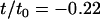, or ∼−20%).

Simulation conditions are identical to those in our earlier work (18), with the exception of the number of membrane lipids, which varies depending on the inclusion radius. Constant vanishing tension, constant temperature Monte Carlo simulations were conducted. Initial conditions were generated as in our earlier work (18): an equilibrated bilayer with 3334 lipids had sufficiently many lipids removed to make room for a given inclusion. The inclusion was then embedded in the membrane and the system was equilibrated (Fig. 2). The average box length was about 〈L〉 = 30 nm for all systems, and the systems contained from 2922 to 3308 lipids, depending on the size of the inclusion. Inclusions were constrained to remain upright (no tilting) to allow for the most elementary comparison to theory.

Analysis of data

At regular intervals throughout the simulation, lipid molecules from the membrane were divided according to their interface bead x and y coordinates into square bins with sides about a molecule wide. The box length fluctuates (slightly) during the course of the simulation, so the bin length does as well, but number of bins (40 per side) was held constant. At any given evaluation, nearly all bins contained exactly two lipid molecules, one from each leaflet.

The thickness (t(x, y) + t₀) for a given square bin was defined as half the vertical distance between the two interface beads. In the event that a bin contained more than one lipid from a given leaflet, the heights of the coleaflet interface beads were averaged before calculating the local distance between opposing leaflets. In the event that a bin contained no lipids from a given leaflet, the height of that leaflet at x, y was estimated using linear extrapolation on neighboring bins. Once t(x, y) was obtained, it was averaged over the polar angle to obtain t(r), and finally t(r) was averaged over the duration of the simulation.

The projected area Σ_pr(x, y) for a given square bin was defined as the average of the projected areas of the molecules contained within. The projected area Σ_pr of a given molecule i was approximated by

(15)

where r_ij is the distance between the interface beads of molecule i and molecule j, projected onto the xy plane, and the sum runs over the six nearest neighbors in the same leaflet. The area deformation profile was averaged like the thickness deformation profile. Equation 15 was verified to reproduce results of more elaborate (triangulation-based) methods to within 1% for several test cases and was adopted for numerical efficiency. The volume deformation profile represents a product of the area and thickness profiles: v(r) + v₀ = (t(r) + t₀)Σ_pr(r).

Derivatives of t(r) at protein contact were calculated by fitting the profile to a fourth order polynomial, constrained to contain the point (r = R, t(R) = t_(R)). The derivative is approximated by the derivative of the polynomial, evaluated at the point of interest (34). The measured derivative could, in principle, depend on the order of the polynomial, the size of the binning window, and the range of the data included in the fit. We avoided making arbitrary decisions for the last two choices by using raw rather than binned data (as recommended in Press et al. (34)), and using the whole profile, rather than a subset close to the inclusion-membrane boundary. The raw unbinned data oscillates over molecular length scales (this is not apparent from the figures in this article, which present binned data) and the fit order should be sufficiently low that these oscillations do not affect the fit. On the other hand, the fit order should be sufficiently high that the important long wavelength features of the profile are captured. Fourth order polynomials were found to simultaneously satisfy both criteria.

SIMULATION RESULTS

An earlier section derived a theory for inclusion-induced deformations that considered the Gaussian curvature and volume perturbations localized to the protein. In this section, we present the actual simulated volume deformation profiles v(r), and discuss both the range and R dependence of the inclusion-induced volume perturbation. We then present measurements on the thickness deformation profiles t(r), and compare them against the analytical predictions made in that earlier section (“Theory”).

Volume deformation

Fig. 3 compares v(r)/v₀ to t(r)/t₀ for both the positive and negative mismatch cases and R = 2.25 nm. The profiles calculated from other values of R are qualitatively similar; quantitative differences are discussed below. v(r)/v₀ has been linearly extrapolated to estimate the volume deformation on the boundary, v_(R)/v₀. The extrapolation is necessary because our binned data only provides the volume deformation a finite distance (one-half bin) away from the boundary. (This is not an issue with the thickness deformation profile because we assume a thickness matching condition: the thickness of a lipid arbitrarily close to the boundary on the lipid side is equal to the thickness of the inclusion. Since we know the thickness of the inclusion, we know the thickness of a lipid on the boundary.)

FIGURE 3.

Volume deformation profile (solid line) and thickness deformation profile (dotted line) measured around inclusions set to have either a positive 10% (left) or negative 20% (right) thickness mismatch with the surrounding membrane; these particular profiles are for inclusions of radius R = 2.25 nm. A solid line connects points that were actually measured, whereas a dashed line indicates a linear extrapolation to the boundary of the protein. Circles mark the boundary of the inclusion; the height of the profile at the boundary is either known in advance (in the case of or extrapolated (in the case of ; see text). The circles marking the estimates of represent the data points used in Fig. 4 for R = 2.25 nm.

Fig. 3 presents v_(R)/v₀ for all studied values of R and both mismatch cases. Regardless of the sign of t_(R), v(r) is always less than zero proximal to the inclusion. The extent of volume nonconservation is considerably larger in the negative mismatch case than the positively mismatched case. In both cases, the magnitude of v_(R) increases with R (Fig. 4); however, in the 10% mismatch case, v_(R) is nearly flat for R ≤ 3.75 nm. This fact will help us in our extraction of k_G and η. We comment that the ratio of volume/thickness immediately yields the area per lipid. The area per lipid in the vicinity of the protein is found to be nearly constant and equal to the equilibrium lipid area of the homogeneous bilayer for the negative mismatch case. In the positive mismatch case, the area is compressed relative to equilibrium.

FIGURE 4.

Lipid volume deformation at inclusion-lipid boundary v_(R)/v₀ as a function of inclusion radius R for inclusions with either a positive 10% or negative 20% thickness mismatch with the surrounding membrane. v_(R)/v₀ was determined using linear extrapolation of v_(R)/v₀ to the boundary, as demonstrated in Fig. 3. As shown in the figure, v_(R)/v₀ is R-dependent, especially in the −20% mismatch case, but the data points in the boxed region are approximated to have constant v_(R)/v₀ for use in the extrapolation scheme presented in Fig. 5 and discussed in the text.

Thickness deformation

To quantitatively compare the thickness deformations to the theory derived in the earlier section, we need to know certain elastic properties of the membrane (k_c, k_G, k_A, c₀, ζ, η). Our earlier work (18) presents some of these parameters, as extracted from homogeneous bilayers composed of the same model lipids used in the work presented here (Table 1). k_c and ζ were calculated by measuring the height and thickness fluctuation spectra, and then fitting the two spectra simultaneously to a theory consistent with that derived in this work. k_A was initially measured the same way, and then adjusted (within the error bars) to reflect some of the outcomes of this work, described below. c₀ was calculated using the stress profile of the homogeneous membrane as described in Safran (27).

TABLE 1.

Elastic properties of membranes formed by the coarse-grained lipids used in this study

Parameter	Value	Description	Reference
t0	2.4 nm	Monolayer thickness	*
Σ0	0.59 nm2	Area per lipid	*
kc	1.4 × 10−19 J	Bilayer bending modulus	*
kG	−0.76 × 10−19 J	2 × monolayer saddle splay modulus	†
	0.94 × 10−19 J nm−4	Bilayer compressibility modulus	*
c0	0.098 nm−1	Monolayer spontaneous curvature	*‡
	0.085 nm−2	Area renormalized spontaneous curvature	*
	−0.78 nm−4	Volume renormalized spontaneous curvature	†

^*Brannigan and Brown (18).

^†Extracted from Fig. 5 of this work.

^‡Brannigan and Brown (18) contains an error. The value reported here is correct.

Beyond the known properties just discussed, this work introduces k_G and η, which also are presumed to be intrinsic properties of the homogeneous bilayer and should, in principle, be measurable from homogeneous simulations. Like c₀, k_G does not appear in the fluctuation spectrum but can in theory be obtained via the stress profile. However, there are ambiguities involved in the stress profile expression. For a tensionless membrane, the integral over the stress profile to obtain c₀ is independent of the location of the origin; this is not the case when one integrates over the stress profile to obtain k_G. In addition, the usual expressions (27) assume the monolayer is deformed as a stack of parallel sheets. Clearly this is not the case of interest in the mismatch problem—the midplane of the bilayer is flat and the interface with water is curved. We did carry out a measurement of k_G as prescribed in Safran (27) using the neutral surface of each monolayer as the origin and obtained k_G = −0.47 k_c. Determination of k_G from experiment or simulation is well known to be a difficult problem (20,35,37), which we do not attempt to solve in this work beyond the estimate obtained from the stress profile (and the alternative linear regression analysis discussed below). The quantity η is related to the derivative of the spontaneous curvature with respect to volume per lipid. Measuring η in a homogeneous bilayer would require a series of simulations with imposed volumes per lipid. Although you might imagine a series of simulations at different pressures to accomplish this, it is impossible to adjust pressure in our solvent-free model. An alternative measurement via volume fluctuations would converge so slowly as to be impractical at present; the large energies associated with volume fluctuations would require exceedingly long sampling times to obtain meaningful results.

As an alternative to obtaining k_G and η from homogeneous simulations, we can extract these parameters based on the theory presented in the earlier section. We have simulated thickness deformation profiles for two sets of proteins with varying R but constant t_(R). For the case of the positively mismatched proteins, we have identified a range of data points with (nearly) constant v_(R) (Fig. 4). The natural boundary condition Eq. 10 suggests a method for collapsing this data and calculating k_G and η as well. Plotting t_rr|_R versus t_r|_R/R for several values of R should yield a line with slope −(k_c + k_G)/k_c and intercept −2(c₀ + ζt_(R)/t₀ − ηv_(R)/v₀). Such a plot is provided in Fig. 5, with the data points corresponding to the boxed points in Fig. 4. The data is noisy but fairly linear. Linear regression yields k_G/k_c = −0.55 ± 0.11 and η/v₀ = −0.78 ± 0.02 nm⁻⁴. The value of k_G is quite close to the measurement from the stress profile, k_G/k_c = −0.47, suggesting that this is a viable method for extracting k_G (and presumably η as well). These values of k_G and η were used in all comparisons to analytical work described in the remainder of this section. Even if we take our procedure for extracting k_G and η to be no more than a glorified process for identifying two fit parameters, it is important to emphasize that these two parameters are used to explain all 14 simulations. The parameters themselves were extracted from only five simulations and do a good job in reproducing the full collection of data.

FIGURE 5.

Boundary curvature plot for positively mismatched systems with five smallest radii (boxed data points in Fig. 4). According to the natural boundary condition (Eq. 10), a plot of t_rr versus t_r/R evaluated at the boundary of inclusions with several different radii R should yield linear data with slope −(k_c + k_G)/k_c and intercept −2(c₀ + ζt_(R)/t₀ − ηv_(R)/v₀). t_rr(R) and t_(R) were measured as described in the section “Simulations: analysis of data”. This plot results in an estimate of k_G/k_c = −0.55 ± 0.11 and η/v₀ = −0.78 ± 0.02 nm⁻⁴.

Observant readers will realize that we use the general boundary condition (Eq. 10) and not the condition specific to a Heaviside function (Eq. 13) in our determination of k_G and η. The general expression is applied because we are analyzing actual simulation data without any additional assumptions. The value of η we obtain may then be used with Eq. 13 in conjunction with the homogeneous Euler-Lagrange equation to provide a good approximation to the simulated deformation profile. Physically, this approximation amounts to assuming a Heaviside volume deformation at the protein boundary (section “Theory”). The theoretical curves discussed below all rely on the Heaviside approximation to allow for analytical solution.

The average thickness deformation profiles t(r)/t₀ for R = 0.75 − 4.5 nm for positive and negative mismatches are shown in Figs. 6 and 7, respectively. In nearly all cases, the membrane slightly “overshoots” the equilibrium thickness; such nonmonotonic behavior has been observed previously (18,21,22) in mesoscopic simulated systems and is consistent with any theory in which the membrane incurs a bending cost from mismatch (8).

FIGURE 6.

Thickness deformation profiles for positively mismatched proteins over a range of radii (R = 0.75 nm to 4.5 nm; data for R = 5.25 nm is not shown due to space constraints but is qualitatively very similar to data for R = 4.5 nm). Circles are actual data from simulation. Solid lines correspond to Eq. 7. Protein mismatch is t_(R)/t₀ = 0.094. Membrane parameters are in Table 1 for the solid lines; dashed lines are the same except k_G = 0 and η = 0, corresponding to the original theory of A-E. For the case of positive mismatch, the theory presented in this article fares similarly to A-E in prediction of the decay profiles.

FIGURE 7.

Thickness deformation profiles for negatively mismatched proteins over a range of radii (R = 0.75 nm to 4.5 nm; data for R = 5.25 nm is not shown due to space constraints but is qualitatively very similar to data for R = 4.5 nm). Circles are actual data points. Solid lines correspond to Eq. 7. Protein mismatch is t_(R)/t₀ = −0.22. Membrane parameters are in Table 1 for the solid lines; dashed lines are the same except k_G = 0 and η = 0, corresponding to the theory of A-E. For this negative mismatch case, the theory presented in this article significantly improves upon the results of A-E.

Also shown are the predictions developed in the Theory section (Eq. 7) with the parameters listed in Table 1. Our initial predictions using the value of reported in our earlier work (18) (12 × 10⁻²⁰ J/nm⁴) consistently predicted that the membrane would return to the unperturbed thickness slightly faster than it does; this is consistent with a measurement of that is too high. The 95% confidence interval on goes down to 9.4 × 10⁻²⁰ J/nm⁴ (see our earlier work (18) and using this value for leads to a better match in all cases. This is the value used in the predictions shown in Figs. 6 and 7 and listed in Table 1.

The predictions neglecting the Gaussian curvature and volume deformations, which correspond to the model of A-E, are shown for comparison (dashed lines in Figs. 6 and 7). Because the Gaussian curvature is only influential for small radius inclusions (as explained in the Theory section), the final panels essentially represent the effect of η alone. Our extension to the theory of A-E does not have a visually significant impact on the predictions for 10% mismatch case. This result is consistent with our earlier observation (18) that 10% mismatch data for one value of R (corresponding to the third panel) was well described by the theory of A-E. Nonetheless, if one looks closely, there is a clear difference in the slopes of the profiles of the two theories as they reach the inclusion boundary. The influence of k_G tends to decrease the contact angle, whereas η increases it for the positive mismatch case. In the first panel of Fig. 4, the effects of k_G and η are actually canceling each other—if we drew one line with k_G turned off and one with η turned off, they would both be distinguishable and on opposite sides of the (indistinguishable) lines currently drawn. (Such lines are not included to keep the figure simple.)

The effects of our extensions to the theory of A-E are much more visible for the −20% mismatch case (Fig. 7). Our predictions (solid line) fit the data very well, whereas if we set k_G and η to zero (dashed line, corresponds to A-E), the prediction returns to the homogeneous value significantly faster than it should for all radii. The theory of A-E also predicts a more substantial overshoot than we observe in simulation. The discrepancies are well outside the error bars of the data and the parameters. The Gaussian curvature is contributing to most (∼80%) of the improvement, relative to A-E, in the prediction for the smallest radius inclusion. The remaining 20% improvement is due to volume nonconservation effects. The role of Gaussian curvature decreases quickly with inclusion radius: it accounts for about half of the improvement for the second smallest radius inclusion, ∼10% of the improvement for the third smallest radius inclusion, and makes an imperceptible contribution to the profile for larger radius inclusions. At the larger radii, the theory presented here improves upon A-E solely because of volume nonconservation effects. For these membranes, the Gaussian curvature plays a larger role for a negatively mismatched inclusion than a positively mismatched inclusion of similar radius due to the sign of the spontaneous curvature. For a positively mismatched inclusion, the spontaneous curvature and the Gaussian curvature work together to flatten the contact angle; for a negatively mismatched inclusion, the spontaneous curvature favors a steep contact angle, whereas the Gaussian curvature still favors a flat one.

FREE ENERGY OF MULTIPLE INCLUSIONS

A complete understanding of the (free) energetics associated with the interaction between multiple inclusions would allow for prediction of the phase behavior in multi-protein assemblies, the equation of state for a two-dimensional fluid of embedded proteins, and related properties associated with a thermodynamic many protein system. Unfortunately, the true energetics of a many protein system include many components, of which the elastic energies considered in this work comprise only a single part. Furthermore, the nature of our model ensures that the interaction energetics between an assembly of proteins is not pairwise additive, which makes a complete understanding of the thermodynamics in just the elastic problem difficult. This section is included to demonstrate two points while largely avoiding the grander questions outlined above. First, it is shown that the effects of Gaussian curvature strongly influence the interactions between inclusions. Second, we demonstrate the nonpairwise additivity of the energies in these systems. These two facts call into question some of the original findings of A-E and lead us to speculate that finite k_G is essential to understanding the aggregation of proteins as seen experimentally.

When calculating the deformation profile around a single inclusion in a large membrane patch (), the details of the boundary conditions far from the inclusion have no effect on the resulting deformation profile (so long as they allow the membrane to relax to equilibrium thickness far from the inclusion). In our analytical calculations of the deformation profiles, we have used the boundary conditions of A-E at L/2 for convenience in calculations and consistency with earlier work. In determining membrane mediated attractions/repulsions among inclusions, however, these boundary conditions are not completely consistent as applied by A-E. Strictly speaking, Eq. 14 corresponds to the free energy of one inclusion-induced deformation when a cylindrical inclusion of radius R is surrounded by a radially symmetric deformation. A-E used this approximate free energy, corresponding to imposing an unwarranted cylindrical symmetry on the problem to estimate the interaction between two proximal inclusions at a separation of L. Compared to exact numerical calculations for the interaction energy between two inclusions, we find the approximate approach generally results in an energy scale that is too large, deviating qualitatively from the exact solution for small inclusion separations. In what follows, energetics were calculated exactly numerically; the approximate analytical scheme of A-E is abandoned for this portion of our work.

Our numerical calculations are similar to those introduced in our earlier work (18). We calculate the elastic interaction energy for any configuration of multiple cylindrical inclusions by minimizing the Hamiltonian of Eq. 2 discretized over a lattice. More precisely, we keep the energy density implied by the integrand of Eq. 2 but use an integration region appropriate to multiple inclusions. In practice, we use a large square region with holes punched out to accommodate the inclusions. There is no longer radial symmetry to the problem and we use general expressions for calculating H, K, etc. The lattice is composed of square lattice sites with an associated height; each site is defined as either a membrane site, an inclusion site, or a membrane-protein boundary site. The membrane sites are free to vary their height in the minimization process; boundary sites remained fixed. Inclusion sites can vary their height, but their variation changes the total system energy only through second derivatives defined at nearby boundary sites. This scheme allows us to fix the height of the inclusion without fixing the membrane slope or curvature at the inclusion boundary. Periodic boundary conditions are assumed for the edges of the lattice; however, the box is always chosen big enough that this choice makes no impact on final results—it is merely a convenient choice for the numerics. For the case of a single inclusion, the numerical scheme reproduces the analytical results of the Theory section.

The role of the Gaussian curvature in membrane-mediated interactions between inclusions was investigated by calculating the free energy of bilayer deformation as a function of inclusion separation. To calculate the pair interaction energy, two circular inclusions of radius R = 0.75 nm were defined in the elastic lattice, with their centers separated by a distance r in the x direction. Separate minimizations were conducted for r ranging from 2R to L_x/2, where L_x, the box length, is chosen such that the inclusions are effectively noninteracting at separations of L_x/2. This procedure provides the membrane-mediated interaction potential energy w(2)(r) between two inclusions:

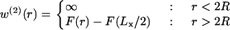(16)

Fig. 8 compares w(2)(r) when k_G is neglected and when k_G is included for the case of negatively mismatched proteins. When k_G is neglected (dashed line), the Hamiltonian corresponds to that of A-E (we choose η = 0 in these simulations to concentrate on Gaussian curvature effects alone). Though we do not assume the radial symmetry of A-E, our qualitative conclusions are very similar so long as k_G is neglected. When two negatively mismatched inclusions reside in a membrane with positive spontaneous curvature, the free energy (neglecting k_G) is minimized when the inclusions assume a finite spacing; dimerization is very unfavorable. This prediction changes dramatically when the Gaussian curvature is added (solid line). With k_G included, dimerization is favored by a few k_BT, although there is still a kinetic barrier to its occurrence.

FIGURE 8.

Two-body potential energy w₂(r) as a function of distance r between two negatively mismatched inclusions. Both lines have η = 0, solid line has k_G as in Table 1, whereas dashed line has k_G = 0 and corresponds to the Hamiltonian of A-E. All other membrane parameters are as in Table 1. Here k_BT corresponds to the temperature used in the coarse-grained molecular simulations of the previous sections (i.e., k_c ∼ 35 k_BT). Protein parameters are R= 0.75 nm, t_(R)/t₀ = −0.20. The theory of A-E predicts that the free energy minimum is achieved at a finite spacing between inclusions, whereas for the theory presented in this article, the free energy minimum is achieved by complete dimerization.

From w(2)(r), we can immediately calculate the second virial coefficient B₂ for a collection of proteins dispersed in a membrane (38):

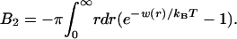(17)

Fig. 9 compares B₂ calculated with η = 0 and k_G = 0 (the Hamiltonian of A-E) and calculated with η = 0 and k_G as in Table 1 over a range of small positive and negative mismatches used in our coarse-grained simulations and commonly used in experiments. In this calculation, k_BT corresponds to the temperature used in the coarse-grained molecular simulations of the previous sections, so, for instance, k_c ∼ 35k_BT. Regardless of whether k_G is considered, B₂ becomes very negative for t_(R)/t₀ > 0.05: inclusions with such mismatches feel a strong attraction that increases with the size of the mismatch. This is consistent with experimental data on bacteriorhodopsin, porin, and other proteins (4,5) that shows that sufficiently mismatched proteins tend to dimerize or aggregate. In fact, B₂ is so negative for t_(R)/t₀ = 0.10 that at the density used in the molecular simulations, the virial expansion is negative at second order.

FIGURE 9.

Second virial coefficient given by Eq. 17 as a function of mismatch, for inclusion with R = 0.75 nm and v_(R)/v₀ = t_(R)/t₀. Membrane parameters are in Table 1, with the following exceptions: dashed line has η = 0, k_G = 0 and consequently represents the Hamiltonian of Aranda-Espinoza et al. (13), and solid line has η = 0 but finite k_G. Here k_BT corresponds to the temperature used in the coarse-grained molecular simulations of the previous sections (i.e., k_c ∼ 35 k_BT).

Experimentally, proteins aggregate at both positive and negative mismatches (4,5), although the magnitude of the critical mismatch is not necessarily the same for both positive and negative cases. In our calculations, it is crucial to include finite k_G to reproduce this qualitative effect. When k_G is neglected, the predicted B₂ is very asymmetric: effective attraction between inclusions increases quickly with positive mismatch magnitude; the attraction at large negative mismatches is only weakly sensitive to mismatch and is actually weaker than the attraction at zero mismatch. This situation is improved significantly by including k_G: when k_G is included, the attraction between inclusions with large negative mismatches is much stronger than the attraction between nonmismatched inclusions, and this attraction is quite sensitive to mismatch magnitude. We comment that A-E extended the arguments presented here by going on to calculate the radial distribution function for a two-dimensional fluid of embedded proteins. We have not attempted this here because our calculations indicate the importance of many-body effects in the elastic energy of mismatched protein assemblies (see below). The treatment presented in A-E assumes two body forces and is not easily extended to the more general case.

An advantage of calculating w(r) numerically, rather than analytically, is that multi-body interactions can also be investigated. For instance, consider two inclusions separated by the minimum separation 2R, and a third separated by distance r from each (see Fig. 10). Multiple lattice simulations (as just described) of this configuration with different values of r were carried out to determine the potential energy of this geometry. Fig. 10 compares the actual potential energy among three inclusions w(3)(r) to the potential energy if it were pairwise additive, i.e., if w(3)(r) = w(2)(2R) + w(2)(r) + w(2)(r). The figure shows that there is a several k_BT difference between these two curves. w(3)(r) is lower than w(2)(2R) + 2w(2)(r) in both the barrier region and the attractive region: it is significantly easier to form a trimer than three dimers. This is just an example of the importance of multi-body effects in determining aggregation and the suitability of this method for their investigation. Studies (24,39) of multi-body effects have previously been carried out for asymmetric inclusions. The work presented here indicates that many-body effects are also important in the case of symmetric but hydrophobically mismatched proteins.

FIGURE 10.

Comparison between three body interaction energy if energy were pair-additive (w(2)(2R) + 2w(2)(r), dashed line) and actual result (w(3)(r), solid line). Inclusions are configured as shown: two inclusions are separated by the minimum spacing and a third is brought toward the dimer while being kept equidistant from each of the other inclusion centers. The solid line does not extend to minimum separation because an equilateral triangle with sides of length 2R is not possible on our square lattice. All parameters are the same as those used for the solid line in Fig. 8.

DISCUSSION

This article presents an extension to the elastic theory of A-E, and most all of our discussion has been directed toward comparison with that model. In earlier work (18), we argued that the handling of boundary conditions and explicit treatment of monolayer spontaneous curvature in the theory of A-E led to the best agreement with simulation and experiment among proposed elastic models in the literature (8,10–15,17). The simulation data supporting this conclusion included fully atomic simulations for the fluctuation spectra of homogeneous membranes and a coarse-grained simulation of the deformation around a single positively mismatched protein inclusion. Upon more extensive simulation of protein inclusions reported on in this work, it became clear that the theory of A-E was not capable of explaining inclusion induced deformations at negative mismatch (at least for our coarse-grained lipid model). The improved theory presented here is capable of fitting the profiles around all 14 of the cylindrical protein shapes we simulated (including the case considered in our earlier work (18)).

The introduction of a finite saddle splay modulus, k_G, and the possibility for lipid volume deformations are both necessary to obtain agreement with simulation over the full range of protein sizes. However, neither of these additions alters the predictions of the model presented in our earlier work (18) in the context of homogeneous bilayer fluctuations over a closed surface. The contribution of Gaussian curvature over a closed homogeneous surface can be rigorously neglected (see next paragraph). Volume fluctuations in the homogeneous bilayer will, at most, lead to renormalization of physical constants already present in the models of A-E and in our earlier work (18). This renormalization should be very slight, due to the large energy scales associated with volume compressibility; only by imposing a large volume perturbation in the mismatched system are significant deviations from v₀ observed. The theory presented here thus improves upon our ability to predict the behavior of inclusion profiles, while leaving unchanged the success of our earlier model in predicting fluctuations in homogeneous systems.

Our treatment of Gaussian curvature energetics seems mathematically unambiguous and physically sound. The energy density of a curved fluid surface should always include such a term, unless by some coincidence the saddle splay modulus is vanishingly small in magnitude (27,28). It is true that this term integrates to a constant (and may thus be ignored for many purposes) if the surface is closed, never changes topology, and is homogeneous in the sense that k_G is everywhere constant (27,28). These conditions are not met for a bilayer with an inserted inclusion. In this article, we consider the membrane surface as ending at the protein boundary, so the surface is not closed. Physically, the situation could also be viewed as a closed surface, but with inhomogeneity in k_G due to the rigidity of the protein. From either perspective, there is no good reason to neglect Gaussian curvature in this problem (although there is a well-established historical precedent for doing so). Readers familiar with differential geometry may be surprised that our expression for the energy of the surface (Eq. 14) does not explicitly display the expected (28) term proportional to k_G times the line integral of the geodesic curvature around the protein boundary. In fact, this omission is only apparent. Equation 14 does include this term, but also includes additional terms with k_G due to the natural boundary conditions assumed in our solution. As written for closest comparison with A-E, everything is jumbled together and the contribution of individual effects is difficult to single out.

In contrast to the question of Gaussian curvature, our treatment of lipid volume deformations is less robust. Although lipid volume is obviously not constant near the protein boundary in simulations, it is not clear how to best include this knowledge in our model. Lacking a theory for the equation of state of an inhomogeneous lipid fluid, we have introduced two major approximations. We assume volume deformations in our system are a given—we do not predict them, but rather extract them from simulation. Further, we approximate the true volume deformation profile with the step profile of Eq. 12. In test cases, we verified numerically that the replacement of the true profile with the step function worked well. It is not clear why this should be the case. The implication is that deformation profiles are much more sensitive to the effect of finite v in the boundary conditions than in the Euler-Lagrange equation itself. We are not aware of prior studies to consider the effects of nonconstant lipid volume. Although simplistic, the approach adopted in this work seems a promising step toward including these important effects in future theories. There is room for improvement along these lines.

The scheme presented for measuring the constants η and k_G relies on our theoretical model, using analytical predictions to fit these two constants over a limited set of our inclusion simulations (those with approximately constant v_(R)). Given the agreement in k_G as obtained from the stress profile calculation and our fitting technique, it is tempting to believe in both the number itself as well as the techniques used to obtain it. Additionally, the numerical value obtained, suggesting the monolayer saddle splay modulus is on the order of the negative monolayer curvature modulus, is in agreement with rough estimates for the behavior of lipid systems (27). It should be stressed, however, that both methods of calculation for k_G are somewhat suspect. The stress profile calculation tacitly assumes a geometry not quite appropriate to our simulations. The linear extrapolation technique relies on a limited set of points and the validity of our elastic model. It is difficult to extract the saddle splay modulus from experiment or simulation (35–37) and we are unaware of a method better than those applied here. There is still work to be done in optimizing a method of calculation for k_G from simulations. Using the definition of η combined with the values reported in Table 1, we conclude that the volume derivative of the spontaneous curvature has the value nm⁻⁴. The positive sign of indicates that the lipids prefer a greater curvature if they have a larger volume (at constant thickness). Since the spontaneous curvature is representative of the shape of the molecule, this suggests that given a larger volume, the lipids assume a more asymmetric or cone-like shape.

It is now becoming possible to stringently test elastic models for membrane phenomena with direct simulations. Simulations are ideally suited to testing analytical theories because the relevant theoretical quantities can be directly inferred from the data. In comparing to experiment, the correspondence is often indirect. This work represents an initial step toward the refinement of analytical models based on simulation data. Further work along similar lines is being pursued.

APPENDIX: SOLUTION TO EQ. 6

Equation 6 was solved using Eq. 12 for the volume profile and Eqs. 8–11 for boundary conditions; the solution was determined both analytically, using Green's function methods, and numerically, using a pseudo-step function. The same solution results from solving the homogeneous form of Eq. 6, but using Eq. 13 instead of Eq. 10 for the natural boundary condition.

For reference, we include the actual expressions for the frequencies

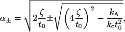(A1)

and coefficients

(A2)

(A3)

(A4)

(A5)

of the solution indicated in Eq. 7. The constants appearing above are defined by

(A6)

and

(A7)

(A8)

We see that introducing k_G complicates matters considerably (Eq. A6 greatly simplifies when k_G = 0), whereas introducing η merely renormalizes the other spontaneous curvature terms.

References

- 1.Lodish, H., D. Baltimore, A. Berk, S. L. Zipursky, P. Matsudaira, and J. Darnell. 1995. Molecular Cell Biology, 3rd ed. Scientific American Books, New York.
- 2.Elliott, J., D. Needham, J. Dilger, and D. Haydon. 1983. The effects of bilayer thickness and tension on gramicidin single-channel lifetime. Biochim. Biophys. Acta. 735:95–103. [DOI] [PubMed] [Google Scholar]
- 3.Kolb, H. A., and E. Bamberg. 1977. Influence of membrane thickness and ion concentration on the properties of the gramicidin a channel. autocorrelation, spectral power density, relaxation and single channel studies. Biochim. Biophys. Acta. 464:127–141. [DOI] [PubMed] [Google Scholar]
- 4.Gil, T., J. H. Ipsen, O. G. Mouritsen, M. C. Sabra, M. M. Sperotto, and M. J. Zuckermann. 1998. Theoretical analysis of protein organization in lipid membranes. Biochim. Biophys. Acta. 1376:245–266. [DOI] [PubMed] [Google Scholar]
- 5.de Planque, M., and J. Killian. 2003. Protein-lipid interactions studied with designed transmembrane peptides: role of hydrophobic matching and interfacial anchoring. Mol. Membr. Biol. 20:271–284. [DOI] [PubMed] [Google Scholar]
- 6.Goulian, M., O. Mesquita, D. K. Fygenson, C. Nielsen, O. Andersen, and A. Libchaber. 1998. Gramicidin channel kinetics under tension. Biophys. J. 74:328–337. [DOI] [PMC free article] [PubMed] [Google Scholar]
- 7.Weiss, T. M., P. C. van der Wel, J. A. Killian, R. E. Koeppe, and H. W. Huang. 2003. Hydrophobic mismatch between helices and lipid bilayers. Biophys. J. 84:379–385. [DOI] [PMC free article] [PubMed] [Google Scholar]
- 8.Huang, H. 1986. Deformation free energy of bilayer membrane and its effects on gramicidin channel lifetime. Biophys. J. 50:1061–1070. [DOI] [PMC free article] [PubMed] [Google Scholar]
- 9.Harroun, T. A., W. T. Heller, T. M. Weiss, L. Yang, and H. W. Huang. 1999. Theoretical analysis of hydrophobic matching and membrane-mediated interactions in lipid bilayers containing gramicidin. Biophys. J. 76:3176–3185. [DOI] [PMC free article] [PubMed] [Google Scholar]
- 10.Helfrich, P., and E. Jakobsson. 1990. Calculation of deformation energies and conformations in lipid membranes containing gramicidin channels. Biophys. J. 57:1075–1084. [DOI] [PMC free article] [PubMed] [Google Scholar]
- 11.Dan, N., P. Pincus, and S. A. Safran. 1993. Membrane-induced interactions between inclusions. Langmuir. 9:2768–2771. [Google Scholar]
- 12.Dan, N., A. Berman, P. Pincus, and S. A. Safran. 1994. Membrane-induced interactions between inclusions. J.Phys. II France. 4:1713–1725. [Google Scholar]
- 13.Aranda-Espinoza, H., A. Berman, N. Dan, P. Pincus, and S. A. Safran. 1996. Interaction between inclusions embedded in membranes. Biophys. J. 71:648–656. [DOI] [PMC free article] [PubMed] [Google Scholar]
- 14.Ring, A. 1996. Gramicidin channel-induced lipid membrane deformation energy: influence of chain length and boundary conditions. Biochim. Biophys. Acta. 1278:147–159. [DOI] [PubMed] [Google Scholar]
- 15.Nielsen, C., M. Goulian, and O. S. Andersen. 1998. Energetics of inclusion-induced bilayer deformations. Biophys. J. 74:1966–1983. [DOI] [PMC free article] [PubMed] [Google Scholar]
- 16.Lundbæk, J. A., and O. Andersen. 1999. Spring constants for channel induced lipid bilayer deformations: Estimates using gramicidin channels. Biophys. J. 76:889–895. [DOI] [PMC free article] [PubMed] [Google Scholar]
- 17.Nielsen, C., and O. S. Andersen. 2000. Inclusion-induced bilayer deformations: effects of monolayer equilibrium curvature. Biophys. J. 79:2583–2604. [DOI] [PMC free article] [PubMed] [Google Scholar]
- 18.Brannigan, G., and F. L. Brown. 2006. A consistent model for thermal fluctuations and protein induced deformations in lipid bilayers. Biophys. J. 90:1501–1520. [DOI] [PMC free article] [PubMed] [Google Scholar]
- 19.Petrache, H., D. Zuckerman, J. Sachs, J. Killian, R. Koeppe, and T. B. Woolf. 2002. Hydrophobic matching mechanism investigated by molecular dynamics simulations. Langmuir. 18:1340–1351. [Google Scholar]
- 20.Chung, H., and M. Caffrey. 1994. The curvature elasticity-energy function of the lipid-water cubic mesophase. Nature. 368:224–226. [DOI] [PubMed] [Google Scholar]
- 21.Venturoli, M., B. Smit, and M. M. Sperotto. 2005. Simulation studies of protein-induced bilayer deformations, and lipid-induced protein tilting, on a mesoscopic model for lipid bilayers with embedded proteins. Biophys. J. 88:1778–1798. [DOI] [PMC free article] [PubMed] [Google Scholar]
- 22.Nielsen, S. O., B. Ensing, V. Ortiz, P. B. Moore, and M. L. Klein. 2005. Lipid bilayer perturbations around a transmembrane nanotube: A coarse grain molecular dynamics study. Biophys. J. 88:3822–3828. [DOI] [PMC free article] [PubMed] [Google Scholar]
- 23.Kandasamy, S., and R. Larson. 2006. Molecular dynamics simulations of model trans-membrane peptides in lipid bilayers: A systematic investigation of hydrophobic mismatch. Biophys. J. 90:2326–2343. [DOI] [PMC free article] [PubMed] [Google Scholar]
- 24.Kim, K. S., J. Neu, and G. Oster. 1998. Curvature-mediated interactions between membrane proteins. Biophys. J. 75:2274–2291. [DOI] [PMC free article] [PubMed] [Google Scholar]
- 25.Braganza, L., and D. L. Worcester. 1986. Structural-changes in lipid bilayers and biological-membranes caused by hydrostatic-pressure. Biochemistry. 25:7484–7488. [DOI] [PubMed] [Google Scholar]
- 26.Weeks, J. D., K. Katsov, and K. Vollmayr. 1998. Roles of repulsive and attractive forces in determining the structure of nonuniform liquids: Generalized mean field theory. Phys. Rev. Lett. 81:4400–4403. [Google Scholar]
- 27.Safran, S. A. 1994. Statistical Thermodynamics of Surfaces, Interfaces and Membranes. Westview Press, Boulder, CO.
- 28.Kamien, R. D. 2002. The geometry of soft materials: a primer. Rev. Mod. Phys. 74:953–971. [Google Scholar]
- 29.Boas, M. L. 1983. Mathematical Methods in the Physical Sciences, 2nd ed. John Wiley & Sons, New York.
- 30.Brannigan, G., P. Philips, and F. L. H. Brown. 2005. Flexible lipid bilayers in implicit solvent. Phys. Rev. E. 72:011915. [DOI] [PubMed] [Google Scholar]
- 31.Sackmann, E. 1995. Physical basis of self-organization and function of membranes: physics of vesicles. In Structure and Dynamics of Membranes, Vol. 1. R. Lipowsky and E. Sackmann, editors. Elsevier Science, Amsterdam, The Netherlands.
- 32.Lindahl, E., and O. Edholm. 2000. Spatial and energetic-entropic decomposition of surface tension in lipid bilayers from molecular dynamics simulations. J. Chem. Phys. 113:3882–3893. [Google Scholar]
- 33.Goetz, R., and R. Lipowsky. 1998. Computer simulations of bilayer membranes: Self assembly and interfacial tension. J. Chem. Phys. 108:7397–7409. [Google Scholar]
- 34.Press, W. H., S. A. Teukolsky, W. T. Vetterling, and B. P. Flannery. 1992. Numerical Recipes in C: The Art of Scientific Computing, 2nd ed. Cambridge University Press, Cambridge.
- 35.Templer, R., J. M. Seddon, and N. A. Warrender. 1994. Measuring the elastic parameters for inverse bicontinuous cubic phases. Biophys. Chem. 49:1–12. [Google Scholar]
- 36.Chung, H., and M. Caffrey. 1994. The curvature elasticity-energy function of the lipid-water cubic mesophase. Nature. 368:224–226. [DOI] [PubMed] [Google Scholar]
- 37.Siegel, D., and M. Kozlov. 2004. The Gaussian curvature elastic modulus of n-monomethylated dioleoylphosphatidylethanolamine:relevance to membrane fusion and lipid phase behavior. Biophys. J. 87:366–374. [DOI] [PMC free article] [PubMed] [Google Scholar]
- 38.McQuarrie, D. A. 2000. Statistical Mechanics. University Science Books, Sausalito, CA.
- 39.Kim, K. S., J. Neu, and G. Oster. 2000. Effect of protein shape on multibody interactions between membrane inclusions. Phys. Rev. E. 61:4281–4285. [DOI] [PubMed] [Google Scholar]