Task-based lens design with application to digital mammography

Abstract

Recent advances in model observers that predict human perceptual performance now make it possible to optimize medical imaging systems for human task performance. We illustrate the procedure by considering the design of a lens for use in an optically coupled digital mammography system. The channelized Hotelling observer is used to model human performance, and the channels chosen are differences of Gaussians. The task performed by the model observer is detection of a lesion at a random but known location in a clustered lumpy background mimicking breast tissue. The entire system is simulated with a Monte Carlo application according to physics principles, and the main system component under study is the imaging lens that couples a fluorescent screen to a CCD detector. The signal-to-noise ratio (SNR) of the channelized Hotelling observer is used to quantify this detectability of the simulated lesion (signal) on the simulated mammographic background. Plots of channelized Hotelling SNR versus signal location for various lens apertures, various working distances, and various focusing places are presented. These plots thus illustrate the trade-off between coupling efficiency and blur in a task-based manner. In this way, the channelized Hotelling SNR is used as a merit function for lens design.

1. INTRODUCTION

The systematic method of lens design in use today is an iterative technique. By this procedure, a basic lens type is first chosen. A paraxial thin-lens and then a thick-lens solution are developed next. Then, with the great progress in computers and applied mathematics today, one can directly go to optimization by relatively high-speed ray trace. Any automatic computer optimization program actually drives an optical design to a local minimum, as defined by a merit function. Broadly speaking, the merit function can be described as a function of calculated characteristics, which is intended to completely describe the value or the quality of a given lens design. The typical merit function is the weighted sum of the squares of many image defects, among which are various aberration coefficients, spot sizes, and modulation transfer function at one or more locations in the field of view. Some merit functions consider the boundary conditions for the lens as well. These boundary conditions include items such as maintaining the effective focal length, center and edge spacings, and overall length. Choice of terms to be included in the merit function is a critical part of the design process. The basis for selecting the aberrations is the experience of designers and their understanding of the nature of lenses and aberrations. The exact choice of term weights and balancing aberrations is largely an empirical process. A large amount of effort has been expended to improve the optimization procedure, but the choice of merit function to provide the best image quality is still not so clear.

Although the aberration coefficients give designers an idea of the performance of the system, the overall effects of these aberrations on the final image is hard to visualize. The question is, what effect does a given amount of aberration have on the performance of optical imaging systems? Phrased in this way, the question is rather vague, and more concrete definitions of image quality are needed. A scientific or medical image is always produced for some specific purpose or task, and the only meaningful measure of its quality is the appropriate observer’s performance on that task. The basic difficulty with the weighted sums of the squared errors as measures of the image quality is that they do not take into account the observer and the task of images. A task-based approach to assessment of image quality must therefore start with a specification of the task followed by a quantitative determination of how well the observer performs the task. Generally, the tasks of practical importance can be either to classify the image into one of two or more categories or to estimate one or more quantitative parameters of the object from the image data. We call these two kinds of tasks classification and estimation, respectively. In astronomical imaging, for example, one might want to detect the presence of a small companion star near a brighter star, or one might want to estimate the relative magnitude of the two stars. The first problem is a classification task, and the second is an estimation task. The observer can be either a human or some mathematical model observer like a machine classifier or pattern recognition system. With the figure of merit for each task, we can quantitatively measure the task-based image quality of imaging systems.

One challenging lens design area is medical x-ray imaging systems, which are usually designed to produce images having the highest quality possible for diagnosis within a specified dose. One type of digital x-ray imaging system uses optics to couple x-ray fluorescent screens onto detection devices or image receptors such as CCD arrays. The lens design must meet a very stringent requirement because the radiation dose applied to patients is limited. Within the safe dose level, x-ray imaging systems should be quantum limited, which means that the dominant noise is the quantum noise from the fluctuation in the x-ray photons. Although x-ray phosphor screens may create hundreds of visible or UV photons per x-ray photon absorbed, the imaging optics cannot couple all of them onto an image receptor. In fact, the number of transmitted light quanta is so much less than the number of those created that the imaging optics can easily become the quantum sink in the whole x-ray imaging system. In its simplest interpretation, when we present an imaging system as a series of cascaded processes or stages, the stage with the fewest quanta per incident x-ray photon is called the quantum sink. The cascaded model is one form of analysis often used by system designers. In this model, the quanta leaving one stage contribute an effective input to the subsequent stage. The starting process usually results from the Poisson statistics characterizing the incident x-ray photons. The randomness introduced by Poisson statistics is a basic noise in photon-limited imaging systems, but there always exists additive noise from external sources, such as electronic components. When imaging systems are designed or assessed, it is important to understand the processes that contribute to the image formation and the effects they have on image signal and noise. In the cascade model, the noise propagates through all stages to the final image as well. All sorts of blurring, especially from aberrations, introduce changes in the appearance and amplitude of the statistical x-ray fluctuations. Such noise takes on a characteristic mottled appearance. Only fast lenses can couple enough light onto image receptors to make recognizable contrast and satisfactory signal intensity over noise. At the same time, the inherent severe aberration of fast lenses can make the mottled appearance even worse.

Recent advances in model observers that predict human perceptual performance now make it possible to optimize optical imaging systems, such as lenses, for human task performance. We illustrate the procedure by investigating a design of a lens for use in an optically coupled digital mammographic imaging system. The cascaded imaging chain consists of a fluorescent screen, an imaging lens, and an electronic imaging device such as a CCD camera. Observers’ performance is evaluated based on the statistical properties of the images from the system. The statistics of images are determined by the statistics of objects and the statistics of the noise from imaging systems. A detailed model of the system to be optimized is described in Section 2. The general observer’s performance and the specific analysis of this model are introduced in Section 3. Section 4 specifies the Monte Carlo strategy used for the numerical computation in evaluating our objective merit function for lens design. Some case studies and discussion are provided in Section 5, and conclusions are presented in Section 6.

2. SYSTEM MODEL

An optically coupled digital mammographic imaging system usually includes an x-ray source, a fluorescent screen, an imaging optical component, and a digital image receiver. A layout drawing of the model system is shown in Fig. 1. Optimizing the imaging optics in this context requires the knowledge of the full system so that the object and the noise propagation can be precisely decided. In Subsections 2.A and 2.B, each system component is investigated carefully and different statistical aspects are given as completely as possible.

Fig. 1.

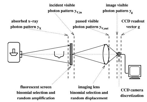
Layout of the model system.

A. Physical System

A remote x-ray generator is placed in front of a fluorescent screen, and the patients to be imaged are in between, usually close to the screen. The detection unit after the screen consists of an optical imaging lens and a CCD camera. The lens images the exit surface of the screen onto the detector plane of the CCD camera.

The most common type of x-ray source in diagnostic radiology is a vacuum tube in which high-energy electrons bombard a metal anode and create x-ray photons. The x-ray photons produced during the exposure are independent of each other, and the total number is Poisson distributed.¹ After the patient, the transmitted x-ray photons still keep their independence since their interactions with tissue are unrelated to each other. The x-ray source is usually far from the fluorescent screen, and there is an antiscattering grid after the patient, so the directions of the x-ray photons are approximately parallel to each other after the patient.

X-ray fluorescent screens are usually made of rare-earth-doped crystallites embedded in plastic binders. These tiny crystal grains emit greenish light upon x-ray excitation. The production rate of light photons is fairly high, over a thousand visible photons per absorbed diagnostic x-ray photon on average. Right after generation, visible light beams are scattered inside the screen by these same crystal grains and meander out to the exit surface of the screen. Once a visible light photon reaches the exit surface, it is most likely displaced from the original position of the absorbed x-ray photon on the surface, and it is also deviated from the original direction of the x-ray photon. The current screen types usually have a reflector on their incident sides to direct more visible light outward. However, the same reflector increases the scattering spread. The detailed specifications of the screens used in the model are based on Kodak products.

An imaging lens couples the exit surface of the screen onto the front surface of a digital imaging detector. To accommodate the whole screen area onto the detector, this lens has to work in a small absolute magnification. The consequently small numerical aperture in the object space cuts off so much visible light emitted from the screen that the ultimate x-ray-to-light-photon conversion rate at the detector stage is around 1, even though 1000 light photons are produced by one x-ray. Making the lens faster while maintaining the field height introduces larger aberrations. Larger aberrations (except distortion) further worsen the blur in the final image. Vignetting can help reduce the off-axis aberrations, but at the same time it causes light loss. The amount of the aberration and the amount of light flux through the lens are coupled with each other.

The last part in the imaging system is a digital imaging detector to produce a discrete set of pixel values representing a continuous image. CCD cameras now have very low noise and very high sensitivity. The electronic noise from CCDs has physical sources independent from other noise previously introduced. In Section 3 we show that it is fairly easy to include any independent noises in the analysis. For now, we analyze an ideal CCD camera with an identical response function for all pixels but no electronic noise. The fill factor of the CCD camera is assumed to be 1.

B. Mathematical Model

The above detailed descriptions and approximations of the physical model system provide us a solid ground to describe mathematically this imaging chain as cascaded stochastic point processes. This type of model for medical imaging is discussed in detail in Ref. 1. The chain begins just in front of the entrance surface of the fluorescent screen and ends at the output of the CCD camera.

1. Point Process of Absorbed X-Ray Photons

In radiography the object is the three-dimensional distribution of the x-ray attenuation coefficient, and the image is the two-dimensional (2D) projection of the x-ray distribution transmitted through that three-dimensional object. To facilitate our analysis of the point processes later in the paper, we use the x-ray distribution transmitted through the patient as the base for the object to our model system. When x-ray beams pass through the fluorescent screen, the crystallites inside the screen absorb a portion of the x rays. Only this portion of the x rays can excite the luminescent crystals to emit visible light and contribute to the image in the CCD camera. We therefore take this portion as the object to the model system and call it f(R), where R is the 2D coordinate on the entrance surface of the screen. Although a realistic x-ray spectrum will introduce energy-dependent absorption coefficients, we think that this detail will not change the results qualitatively: The trends of the signal-to-noise ratio (SNR) curves and the orders of them in the various figures should remain the same, although the exact values can be different. An artificially monochromatic x-ray source is used in our study for the sake of computational simplicity. When we assume that the x-ray source is monochromatic, this object f(R) can also be interpreted as the x-ray number fluence in units of mean number of photons per unit area. The energy fluence for a source is defined as the radiant energy per unit area in radiological imaging, and this quantity is called exposure in photography. The object is thus calculated from the energy fluence divided by the energy of each x-ray photon. Our object is in fact the noise-free x-ray pattern. If we take into account all the patients to be imaged, the object is a random function sampled from the ensemble of patients. Each object produces a noisy x-ray pattern. This x-ray pattern can be described as a 2D Poisson point process, where each x-ray photon contributes in the process a randomly located delta function on the entrance surface of the screen. The photons all propagate in the same direction that we denote as the +z axis in the three-dimensional coordinate system. The entrance surface of the screen therefore lies in the x, y plane. Similar to the situation in patients, every x-ray photon interacts independently of all the other photons within the screen. The absorbed portion of the x-ray photons comprises another random point process that follows Poisson statistics. Mathematically speaking, the absorption mechanism is a binomial selection of the incident point process, and the binomial selection of a Poisson process is still a Poisson with a modified mean.¹ The mean of the Poisson process resulting from the absorption is the object.

Now we are ready to describe the initial random process in the imaging chain. It is the Poisson point process for any given object f(R). This random process models both the object and the noise before the whole imaging system. A sample function of this first random process can be written as

$$y_x(R)=\sum _{n=1}^N\delta (R-R_n),$$ (2.1)

where R_n is the 2D position vector in the entrance surface of the screen at which the nth x-ray photon hits, and each delta function describes an x-ray photon passing through the patient and absorbed by the screen. The x-ray object f(R) is a random function drawn from the ensemble of objects to be imaged, so this process is actually a doubly stochastic Poisson process.¹ For any given object, the total number of absorbed x-ray photons N is a Poisson random variable, whose mean is the integral of the process mean f(R). The integral is over the support of the object, which is usually the whole area of the screen: N

$$\overline{N}(f)=\int {\int }_{\text{supp}}{\text{d}}^{2}Rf(R).$$ (2.2)

Because of the independence of the photons in the Poisson process, the probability density function (PDF) of R_n is just the properly normalized process mean function:

$${\text{pr}}_R(R_n|f)=\frac{f(R_n)}{\overline{N}(f)}=\frac{f(R_n)}{\int {\int }_{\text{supp}}{\text{d}}^{2}Rf(R)}.$$ (2.3)

This 2D point process does not include the third spatial coordinate of the absorbed x-ray photons z, which is the absorption depth. The screen should have a uniform response over its area when well manufactured. The absorption depth z_n of the nth absorbed x-ray photon is thus independent of its 2D position R_n. Given the characteristic x-ray absorption depth d_x, the absorption depth z_n follows the exponential law within the screen thickness d:

$${\text{pr}}_Z(z_n)=\frac{1}{d_x}\frac{exp(-z_n/d_x)}{1-exp(-d/d_x)},\hspace{0.17em}0\le z_n\le d.$$ (2.4)

The proportion of the absorbed x rays in the x-ray pattern after the patient is 1 − exp(−d/d_x).

The 2D point process of the absorbed x-ray photons, together with the PDF of the absorption depth, forms the complete mathematical description of the first stage in the cascaded imaging system model.

2. Point Process of Incident Visible Photons

Once an x-ray photon is absorbed, some of its energy is then re-emitted in the form of fluorescent light photons. Each absorbed x-ray photon can produce more than a thousand visible light photons on average. The initial x-ray interactions with the fluorescent crystals most likely produce high-energy photoelectrons. A high-energy electron migrating through inorganic scintillator crystallites inside the screen will form a large number of electron–hole (e–h) pairs. An e–h pair quickly recombines and independently emits a visible photon with high probability. The e–h pair sites are all so close together near the primary absorption site of the x-ray photon that all the excited visible lights can be considered as emitting from the absorption site. In fact, the e–h pair range is of the order of 2 μm in the mammographic energy range. After demagnification by the lens, the images of the e–h pair ranges are much smaller than the pixel size in common CCD cameras, which is of the order of tens of micrometers. The visible photons propagate equally probably in all directions upon creation. This simplified light conversion model is the starting point of the visible light scattering. The visible light photons are scattered by the tiny crystals in the screen and may be reflected by the diffuse reflectors on the back of the screen. Before they can get out of the screen, they have a slight chance of being absorbed along the way. The result of the scattering analysis follows next.

The whole process can be described mathematically as a random amplification process with x-ray photons as primaries and visible photons that get out of the exit surface of the screen as secondaries.^1–3 The amplification number of each absorbed x-ray photon is random. The nth primary produces K_n secondaries, and we can write down a sample function of the 2D stochastic process after this amplification mechanism:

$$\begin{array}{l}{y}_{v,\text{in}}(r)=\sum _{n=1}^N\sum _{k=1}^{K_n}\delta \hspace{0.17em}(r-r_{nk})\\ =\sum _{n=1}^N\sum _{k=1}^{K_n}\delta \hspace{0.17em}(r-R_n-\mathrm{\Delta }{r}_{nk}),\end{array}$$ (2.5)

where r_nk is the location on the exit surface of the screen for the kth secondary produced by the nth primary and Δr_nk is the random displacement. The position vectors here and in the rest of the paper are all 2D. They may be on different planes along the optical axis, but all the planes are parallel to each other and have identical coordinate systems with the origins on the optical axis. When projected along the optical axis on a certain plane, position vectors follow the common 2D vector arithmetic correctly.

In radiometry, a function called the bidirectional transmission distribution function [(BTDF) (r, $\widehat{s},{\widehat{s}}^{\prime }$)] is used to quantify the directional property of light transmission through a thin transmissive layer.¹ It is defined as the ratio of transmitted radiance in the direction $\widehat{s}$ to the radiant incidence at the position r on the layer. Radiant incidence is the irradiance of a highly collimated beam traveling in the direction ${\widehat{s}}^{\prime }$ so the BTDF actually specifies the transmitted radiance generated by such a beam. The BTDF is in units of inverse steradians, and we can relate the transmitted radiance with the incident radiance by the following integral:

$$L_{\text{trs}}(r,\widehat{s})=\int {\int }_{2\pi }\text{d}{\mathrm{\Omega }}^{\prime }\text{BTDF\hspace{0.17em}(}r,\widehat{s},\hspace{0.17em}{\widehat{s}}^{\prime })L_{\text{inc}}(r,{\widehat{s}}^{\prime })cos({\theta }^{\prime }),$$ (2.6)

where the integral is over the hemisphere of unit vector ${\widehat{s}}^{\prime }$ directed toward the surface, and $\widehat{s}$ lies in the same hemisphere. Here we assume that the visible photons all have the same energy and, with the above assumption of monochromatic x-ray sources, the radiometric quantities of x ray and visible light can be defined in units of photon numbers.

Now we generalize the conventional BTDF to describe the entire light transmission through the fluorescent screen. For thick translucent objects like screens, the generalized BTDF is also a function of the position vector on the exit surface r′, namely, BTDF (r, $\widehat{s}$; r′, ${\widehat{s}}^{\prime }$). The light-transmission process includes two steps: (1) the amplification process in which the absorbed x-ray photons are converted into a larger number of visible light photons and (2) the scattering process in which the visible light photons are displaced from the original x-ray absorption sites on the exit surface of the screen. In this analysis, the incident light is the absorbed x rays, and the transmitted light is the visible light out of the screen. Because the transmitted light displacement distribution can be different at different incident x-ray absorption depths, the generalized BTDF should also be a function of depth z. The generalized BTDF is thus similarly defined as the ratio of transmitted radiance in the direction $\widehat{s}$ at the position r on the exit plane to the radiant flux on the entrance plane when the incident x-ray is absorbed at the depth z. Radiant flux is the flux of highly collimated x rays traveling in direction ${\widehat{s}}^{\prime }$ with a pointlike size at the position r′ on the entrance plane. Hence the generalized BTDF, by definition, is in units of inverse steradians per square meters, suggesting that it can be used in an integral over a solid angle and a 2D spatial vector. In fact, it is the kernel of the integral relating incident radiance to the transmitted radiance if the absorption happens at depth z:

$$\begin{array}{l}{L}_{\text{trs}}(r,\widehat{s}|z)=\int {\int }_{2\pi }\text{d}{\mathrm{\Omega }}^{\prime }\hspace{0.17em}{\int }_{\infty }{\text{d}}^{\text{2\hspace{0.17em}}}R\text{BTDF\hspace{0.17em}}\\ \times \hspace{0.17em}(r,\hspace{0.17em}\widehat{s},\hspace{0.17em}R,\hspace{0.17em}{\widehat{s}}^{\prime }|z)L_{\text{inc}}(R,\hspace{0.17em}{\widehat{s}}^{\prime })cos({\theta }^{\prime }),\end{array}$$ (2.7)

where all the radiometric quantities are in units of photon numbers. Therefore the mean gain of the amplification process is automatically incorporated into the generalized BTDF.

In our model, the incident radiance is an angular delta function scaled by the absorbed x-ray irradiance. Because we assume that x rays have normal incidence on the screen, the direction cosine is 1. The delta function is along the propagating direction ${{\widehat{s}}^{\prime }}_0$ of all the x-ray photons, which is parallel to the optical axis, defined in the $+\widehat{z}$ direction:

$$L_{\text{inc}}(R,\hspace{0.17em}{\widehat{s}}^{\prime })=\frac{M_{\text{inc}}(R)\delta (\hspace{0.17em}{\widehat{s}}^{\prime }-{{\widehat{s}}^{\prime }}_0)}{cos({\theta }^{\prime })}=M_{\text{inc}}(R)\delta (\hspace{0.17em}{\widehat{s}}^{\prime }-\widehat{z}),$$ (2.8)

where M_inc is the absorbed incident x-ray irradiance on the entrance surface at the position R. By applying Eq. (2.7), it is easy to get the transmitted visible light radiance at the absorption depth z:

$$L_{\text{trs}}(r,\hspace{0.17em}\hspace{0.17em}\widehat{s}|z)=\int {\int }_{\infty }{\text{d}}^{\text{2}}R{M}_{\text{inc}}(R)\text{BTDF}(r,\widehat{s},r^{\prime },\widehat{z}|z).$$ (2.9)

The subsequent irradiance on the exit surface can be found by integrating the irradiance over all directions in the forward hemisphere:

$$\begin{array}{l}{M}_{\text{trs}}(r|z)=\int {\int }_{2\pi }\text{d}\mathrm{\Omega }{L}_{\text{trs}}(r,\hspace{0.17em}\widehat{s}|z)cos(\theta )\\ \int {\int }_{\infty }{\text{d}}^{2}R{M}_{\text{inc}}(R)\int {\int }_{2\pi }\text{d}\mathrm{\Omega }\text{BTDF}\\ \times (r,\widehat{s},\hspace{0.17em}R,\widehat{z}|z)cos(\theta ).\end{array}$$ (2.10)

The kernel that relates incident irradiance to transmitted irradiance can also be called the irradiance point response function (PRF), which is

$$\text{PRF(}r,R|z)=\int {\int }_{2\pi }\text{d}\mathrm{\Omega }\text{BTDF\hspace{0.17em}(}r,\widehat{s},\hspace{0.17em}R,\hspace{0.17em}\widehat{z}|z)\hspace{0.17em}cos(\theta ).$$ (2.11)

When in photon number units, the irradiances are equivalent to the mean processes f of the corresponding random point processes:

$$M_{\text{inc}}(R)=f(R),\hspace{0.17em}\hspace{0.17em}\hspace{0.17em}{M}_{\text{trs}}(r|z)=f^{\prime }(r).$$ (2.12)

The amplification PRF p_d can be derived from the irradiance PRF in Eq. (2.11):

$$\begin{array}{l}{p}_d(r,\hspace{0.17em}R|z)=\int {\int }_{2\pi }\text{d}\mathrm{\Omega }\text{BTDF(}r,\hspace{0.17em}\widehat{s},\hspace{0.17em}R,\hspace{0.17em}\widehat{z}|z)cos(\theta )\\ =\overline{k}(R|z)\cdot {\text{pr}}_{\mathrm{\Delta }r}(\mathrm{\Delta }r|R,\hspace{0.17em}z).\end{array}$$ (2.13)

As shown in Ref. 1, the amplification PRF determines both the PDF of the displacement position pr_Δr and the average gain $\overline{K_n}$ by

$${\text{pr}}_{\mathrm{\Delta }r}(\mathrm{\Delta }r|R,\hspace{0.17em}z)=\frac{p_d(R+\mathrm{\Delta }r,\hspace{0.17em}R|z)}{\overline{K_n}(R|z)},$$ (2.14)

$$\overline{K_n}(R|z)=\int {\int }_{\infty }{\text{d}}^{2}r{p}_d(r,\hspace{0.17em}R|z),$$ (2.15)

where $\overline{K_n}$ is the average number of secondaries per primary. We also note that the average number of secondaries per primary is independent of the particular primary, or n, and can be written as $\overline{K}$. Similarly, the PRF in the four-dimensional space (the 2D position and the 2D direction) is the generalized BTDF in photon number units corrected by the direction cosine:

$$\text{PRF(}r,\widehat{s},\hspace{0.17em}R,\hspace{0.17em}\widehat{z}|z)=\text{BTDF\hspace{0.17em}(}r,\hspace{0.17em}\widehat{s},\hspace{0.17em}R,\hspace{0.17em}\widehat{z}|z)cos(\theta ).$$ (2.16)

The joint PDF of the exit position and direction of a scattered secondary photon is thus the normalized four-dimensional PRF:

$$\text{pr(}r,\hspace{0.17em}\widehat{s}|R,\hspace{0.17em}z)=\frac{\text{BTDF\hspace{0.17em}(}r,\hspace{0.17em}\widehat{s},\hspace{0.17em}R,\hspace{0.17em}\widehat{z}|z)cos(\theta )}{\overline{K}(R|z)}.$$ (2.17)

The conditional PDF of the outgoing direction can be derived from the joint PDF of Eq. (2.17). The direction is determined by the azimuth angle φ and the polar angle θ. The differential solid angle in the angular space is in fact the product of the differential azimuth angle dφ and the differential cosine of the polar angle d cos(θ). The direction PDF is thus expressed as the joint PDF of the azimuth angle φ and the cosine of the polar angle cos(θ). The conditional PDF of the outgoing direction is expressed as

$$\begin{array}{l}\text{pr(\hspace{0.17em}}\widehat{s}|\mathrm{\Delta }r,\hspace{0.17em}R,\hspace{0.17em}z)\\ =\frac{\text{pr(}R+\mathrm{\Delta }r,\hspace{0.17em}\widehat{s}|R,\hspace{0.17em}z)}{\text{pr(\hspace{0.17em}}\mathrm{\Delta }r|R,\hspace{0.17em}z)}\\ =\frac{\text{BTDF(}R+\mathrm{\Delta }r,\hspace{0.17em}\widehat{s},\hspace{0.17em}R,\hspace{0.17em}\widehat{z}|z)cos(\theta )}{\int {\int }_{2\pi }\text{d}{\mathrm{\Omega }}^{\prime }\hspace{0.17em}\text{BTDF(}R+\mathrm{\Delta }r,\hspace{0.17em}{\widehat{s}}^{\prime },\hspace{0.17em}R,\hspace{0.17em}\widehat{z}|z)cos({\theta }^{\prime })}.\end{array}$$ (2.18)

The conditional direction PDF of Eq. (2.18) is completely determined by the generalized BTDF, but the PDF of the gain is still unknown except for the mean value. The amplification mechanism removes the independence among the different points in the resultant process because two or more secondaries can be produced by one primary. Shift invariance holds inside the boundary of well-manufactured screens, where the secondary displacement PDF [Eq. (2.14)] and the conditional direction PDF [Eq. (2.18)] are both independent of the primary position R. The PRF p_d(r, R|z) is now only a function of the displacement r − R and the depth z, and it can be called the point-spread function. The secondaries from different primaries are independently produced since the screen should have no memory from one primary to another. The multivariate density on {Δr_nk} is therefore a product of univariate densities on each of the Δr_nk. The product form is also valid for the multivariate density on {(Δr_nk, ${\widehat{s}}_{nk}$)} and the conditional multivariate density on { ${\widehat{s}}_{nk}$|Δr_nk}. Similarly, the conditional multivariate density pr({r_nk}|R_n) is the product of the univariate densities pr(r_nk|R_n).

3. Point Process of Output Visible Photons

The visible light from the screen has to pass through the optical imaging lens after the screen to contribute to the image formation on the CCD camera. Because of the limited entrance pupil and the complicated vignetting effect of the lens, each visible photon has only a small chance to pass. The passing probability pass(R + Δr, R|z) of an output visible photon depends on its exit position R + Δr and its primary position R. On the basis of the probability densities above, the function pass(R + Δr, R|z) can be obtained from the generalized BTDF function:

$$\begin{array}{l}\text{pass(}R+\mathrm{\Delta }r,\hspace{0.17em}R|z)\\ =\int {\int }_{\mathrm{\Omega }(R+\mathrm{\Delta }r)}\text{d}\mathrm{\Omega }\text{pr(}\widehat{s}|\mathrm{\Delta }r,\hspace{0.17em}R,\hspace{0.17em}z)\\ =\frac{\int {\int }_{\mathrm{\Omega }(R+\mathrm{\Delta }r)}\text{d}\mathrm{\Omega }\text{BTDF(}R+\mathrm{\Delta }r,\hspace{0.17em}\widehat{s},R,\hspace{0.17em}\widehat{z}|z)cos(\theta )}{\int {\int }_{2\pi }\text{d}\mathrm{\Omega }\text{BTDF(}R+\mathrm{\Delta }r,\hspace{0.17em}\widehat{s},R,\hspace{0.17em}\widehat{z}|z)cos(\theta )},\end{array}$$ (2.19)

where the solid angle Ω(R + Δr) incorporates only the directions that a visible photon can pass through the lens from the position R + Δr on the exit surface of the screen. The solid angle is determined by the lens pupil and vignetting at the field R + Δr. This binomial selection mechanism needs to be explicitly expressed because the input process is no longer a Poisson process. One sample function of the resultant process is

$$y_{v,\text{out}}(r)=\sum _{n=1}^N\sum _{k=1}^{K_n}{\beta }_{nk}\delta (r-R_n-\mathrm{\Delta }{r}_{nk}),$$ (2.20)

where β_nk is a random variable taking only two values: It is 0 when the kth visible photon produced by the nth x-ray photon does not pass through the lens or 1 when the photon reaches the CCD camera. The probability law on β_nk is

$$\begin{array}{l}Pr({\beta }_{nk}|R_n,\mathrm{\Delta }{r}_{nk},z_n)\\ =\{\begin{array}{ll}\text{pass\hspace{0.17em}(}{R}_n+\hspace{0.17em}\mathrm{\Delta }{r}_{nk},R_n|z_n),\hfill & {\beta }_{nk}=1\hfill \\ \text{1}-\text{pass\hspace{0.17em}(}{R}_n+\hspace{0.17em}\mathrm{\Delta }{r}_{nk},R_n|z_n),\hfill & {\beta }_{nk}=0\hfill \end{array}.\end{array}$$ (2.21)

Each visible photon travels independently inside the lens, so the multivariate density on {β_nk} is the product of the univariate densities on each β_nk.

4. Point Process of Visible Photons in the Image

Because of aberrations, each passed visible photon is displaced from the ideal image position on the image plane. For a given photon (or ray) direction, this deviation is deterministic, but the photon directions are random. Thus aberrations translate randomness of the incident directions $\widehat{s}$ starting from the position r on the exit surface of the screen into randomness of the position displacements Δr″ away from the ideal image positions r″ on the CCD detector surface. Another 2D spatial stochastic process is produced by this translated randomness.⁴ A sample function of this process is

$$y_g^{\prime }(r^{″})=\sum _{n=1}^N\sum _{k=1}^{K_n}{\beta }_{nk}\delta (r^{″}-{r^{″}}_{nk}),$$ (2.22)

where r″_nk is the position on the detector plane of the kth visible photon produced by the nth x-ray photon.

Because of the magnification of the lens, ideal image positions are generally not the same as the corresponding object positions. We can properly scale the sample functions on the CCD detector plane to cancel the image magnification. In particular, every position vector is divided by the magnification so that the ideal image points coincide with the corresponding object points. The resultant sample function is expressed as

$$\begin{array}{l}{y}_g(r^{\prime })=\sum _{n=1}^N\sum _{k=1}^{K_n}{\beta }_{nk}\delta (r^{\prime }-{r^{\prime }}_{nk})\\ =\sum _{n=1}^N\sum _{k=1}^{K_n}{\beta }_{nk}\delta (r^{\prime }-R_n-\mathrm{\Delta }{r}_{nk}-\mathrm{\Delta }{r^{\prime }}_{nk}),\end{array}$$ (2.23)

where Δr′_nk is the scaled displacement from the scaled ideal image point position that is the same as the object point R_n + Δr_nk. This scaled process again can be treated as a particular random amplification process with the nonrandom gain equaling 1. The PDF of the displacement equals its PRF p_g(r′, r|R, z):

$$p_g(R+\mathrm{\Delta }r+\mathrm{\Delta }{r}^{\prime },\hspace{0.17em}R+\mathrm{\Delta }r|R,z)={\text{pr}}_{\mathrm{\Delta }{r}^{\prime }}(\mathrm{\Delta }{r}^{\prime }|R,\hspace{0.17em}\mathrm{\Delta }r,\hspace{0.17em}z).$$ (2.24)

We note that the PRF is not the properly scaled continuous spot diagram from optical design softwares such as CODEV or ZEMAX; the spot diagram is generated from the particular incident direction distribution density that is uniform in the direction tangent. Nor can we compute the PRF from the product of the spot diagram and the actual PDF of the direction. Analytically, we can employ the transformation law to get the PDF of Δr′ from the PDF of the $\widehat{s}$ inside the passing cone Ω(R + Δr). For a given lens, any displacement Δr′ depends on the object point position r and the incident direction $\widehat{s}$ before the lens:

$$\mathrm{\Delta }{r}^{\prime }=\mathrm{\Delta }{r}^{\prime }(\widehat{s},\hspace{0.17em}r)=\mathrm{\Delta }{r}^{\prime }(\widehat{s},\hspace{0.17em}R+\mathrm{\Delta }r).$$ (2.25)

We should be aware that the conditional direction PDF inside the passing cone is the original PDF normalized by the probability to be inside the cone:

$$\begin{array}{l}{\text{pr}}_{\widehat{s}}\text{(\hspace{0.17em}}\widehat{s}|R,\mathrm{\Delta }r,\hspace{0.17em}z)\\ =\frac{\text{BTDF(}R+\mathrm{\Delta }r,\hspace{0.17em}\widehat{s},\hspace{0.17em}R,\hspace{0.17em}\widehat{z}|z)cos(\theta )}{\int {\int }_{\mathrm{\Omega }(R+\mathrm{\Delta }r)}\text{d}{\mathrm{\Omega }}^{\prime }\hspace{0.17em}\text{BTDF(}R+\mathrm{\Delta }r,\hspace{0.17em}\widehat{s},\hspace{0.17em}R,\hspace{0.17em}\widehat{z}|z)cos({\theta }^{\prime })}.\end{array}$$ (2.26)

When finding the mean value of some function of the displacement u(Δr′), we obtain the integral relation between the point-spread function p_g and the conditional direction PDF as

$$\begin{array}{l}\int {\int }_{\infty }{\text{d}}^2\mathrm{\Delta }{r}^{\prime }u(\mathrm{\Delta }{r}^{\prime }){\text{pr}}_{\mathrm{\Delta }{r}^{\prime }}(\mathrm{\Delta }{r}^{\prime }|R,\hspace{0.17em}\mathrm{\Delta }r,z)=\int {\int }_{\mathrm{\Omega }(R+\mathrm{\Delta }r)}\text{d}\mathrm{\Omega }u[\mathrm{\Delta }{r}^{\prime }(\widehat{s},r)]\text{pr(}\widehat{s}|R,\hspace{0.17em}\mathrm{\Delta }r,\hspace{0.17em}z)\\ =\frac{\int {\int }_{\mathrm{\Omega }(R+\mathrm{\Delta }r)}\text{d}\mathrm{\Omega }u[\mathrm{\Delta }{r}^{\prime }(\widehat{s},r)]\text{BTDF(}R+\mathrm{\Delta }r,\hspace{0.17em}\widehat{s},\hspace{0.17em}R,\hspace{0.17em}\widehat{z}|z)cos(\theta )}{\int {\int }_{\mathrm{\Omega }(R+\mathrm{\Delta }r)}\text{d}{\mathrm{\Omega }}^{\prime }\hspace{0.17em}\text{BTDF(}R+\mathrm{\Delta }r,\hspace{0.17em}{\widehat{s}}^{\prime },\hspace{0.17em}R,\hspace{0.17em}\widehat{z}|z)cos({\theta }^{\prime })},\end{array}$$ (2.27)

where the direction $\widehat{s}$ is chosen inside the passing cone Ω (R + Δr). Whenever the angular space of passed $\widehat{s}$ is mapped onto the Δr′ space, this integral relation is always true. We do not usually know the analytical expression of Δr′( $\widehat{s}$,r) or r′ ( $\widehat{s}$,r), but we can find precisely r′ ( $\widehat{s}$,r) with Snell’s law and geometric optics. Given a group of randomly emanating photons corresponding to proper direction density, computers can trace them through the lens onto the CCD detector plane and automatically produce the requested sample of the above formidable PDF of the scaled final displacement on the CCD.

5. Random Image Vector

The last step is to map this 2D continuous image function y_g(r′) into a 2D discrete image array g. Remember that we ignore the electronic noise from the CCD for now, so the final image array is

$$\begin{array}{l}g=\{g_m,m=\{1,1\},\{1,2\},\dots ,\{M,\hspace{0.17em}M\left\}\right\},\\ g_m=\int {\int }_{\text{supp}}{\text{d}}^{\text{2}}{r}^{\prime }g(r^{\prime })h_m(r^{\prime }),\end{array}$$ (2.28)

where h_m(r′) is the response function of the mth pixel. This mapping from a continuous function to a discrete vector can be denoted by a discretization operator D:

$$g=D{y}_g,$$ (2.29)

$${[D{y}_g]}_m=\int {\int }_{\text{supp}}{\text{d}}^{\text{2}}{r}^{\prime }{y}_g(r^{\prime })h_m(r^{\prime }).$$ (2.30)

Under the ideal CCD model, the response function is the 2D rectangle function centered at the corresponding pixel with the size of the pixel. Every response function has the same size, and adjacent response functions have no gap in between.

3. MERIT FUNCTION

Improving image quality is the central goal for imaging system optimization such as lens design. A task-based assessment of image quality is rooted in statistical decision theory, where the observer performance in the specific task is used to measure the image quality. The major type of task of a mammographic imaging system is to help diagnose breast tumors, which is a classification task. Therefore the measure of the observer performance in the classification task can be used as the merit function for optimizing lens design.

A. Observer Performance

The observer is the strategy by which the task gets done. Both human and computer algorithms can perform classification tasks, and the algorithms are called mathematical observers. Mathematical observers calculate the outcome from some operation on the data, and the outcome is called the test statistic. In addition to the test statistic, mathematical observers also have a rule of dividing the data space into several regions without ambiguity based on the test statistic. Each region corresponds to a class or hypothesis.

For a general L-class task, the Bayesian observer has complete knowledge of the statistical information regarding the task and uses that knowledge to make the best decision. Thus the performance of the Bayesian observer provides an upper bound for all the other observer performances. It is also called the ideal observer. The test statistic of the ideal observer (the likelihood ratio) is usually nonlinear in the data and difficult to implement. Another type of observer has the linear test statistic t = W^tg in the data g, and the template W is a matrix. The Hotelling observer is the optimal linear observer in the sense that it maximizes the Hotelling trace. The Hotelling trace is a useful performance measurement that calculates the separability of the classes. The expression of the Hotelling trace in a two-class case is given in this section.

The first task of mammographic imaging systems is to make the decision between two hypotheses: tumor-present H₁ and tumor-absent H₀. For this binary or two-class task, every mathematical observer uses a scalar test statistic t and compares it with a threshold t_c. The observer makes decision D₁ when the statistic is larger than the threshold; otherwise, the observer makes decision D₀. The conditional probability Pr(D₁|H₁) is called the true positive fraction, and Pr(D₁|H₀) is called the false positive fraction; they are both functions of the threshold. We can plot the true positive fraction versus the false positive fraction with the threshold as the changing parameter. The plot is referred to as the receiver operating characteristic (ROC) curve. The area under the ROC curve (AUC) can also be used as a performance measure. The Hotelling observer for the binary detection task has the template vector w as follows:

$$w=K_g^{-1}\mathrm{\Delta }\overline{g},$$ (3.1)

$$K_g=\frac{1}{2}(K_1+K_0),$$ (3.2)

$$\mathrm{\Delta }\overline{g}={\overline{g}}_1-{\overline{g}}_0,$$ (3.3)

where K₁, K₀, ${\overline{g}}_1$, and ${\overline{g}}_0$ are the covariance matrices and the mean image vector under each hypothesis, respectively. The Hotelling trace is now $J_{\text{Hot}}=4\mathrm{\Delta }{\overline{g}}^t{K}_g^{-1}\mathrm{\Delta }\overline{g}$. We define a new performance measure called the Hotelling SNR as a quarter of the Hotelling trace:

$${\text{SNR}}_{\text{Hot}}^{\text{2}}=\mathrm{\Delta }{\overline{g}}^t{K}_g^{-1}\mathrm{\Delta }\overline{g}.$$ (3.4)

Only the first and second moments of the data appear in the SNR definition, which relaxes the requirement for the full conditional probabilities needed in the AUC calculation. When the test statistic is Gaussian distributed under both hypotheses, the AUC can be monotonically mapped to the SNR. The mapping is through the error function

$${\text{SNR}}_{\text{Hot}}=2\hspace{0.17em}{\text{erf}}^{-\text{1}}(2\times \text{AUC}-1).$$ (3.5)

For non-Gaussian test statistics, the result of this mapping is called the detectability index d_A.

Observers for the tumor detection task are usually radiologists who look at the images formed by the mammographic system. The human observer’s AUC under this task can be measured from psychophysical studies. This experiment is limited by the resources and is very time-consuming. We need a mathematical observer to model the human observer to facilitate the performance measurement. The ROC curve and the AUC are used to compare the models. The channelized Hotelling observer is a computationally feasible model whose ROC curve correlates well with that of the human observer. The channelized Hotelling observer was first introduced to medical image quality assessment by Myers and Barrett.⁵ On the basis of previous work in our group,⁶ the channelized Hotelling observer can satisfactorily predict the human observer performance in a wide range of situations when the tumor profile is deterministic. The notion of channels in the human visual system has been studied intensively in vision science for many years.⁷ Gabor functions are widely used as one type of channel set. Several other kinds of functions have been used instead of Gabor functions. Difference of Gaussians (sometimes called DOGs),^8,9 a Gaussian-derivative model,¹⁰ the Laplacian operator,¹¹ and Cauchy functions¹² have all been used in the research. On the basis of these studies in vision research, the introduction of the channels into the model of the human observer has been successful in a variety of circumstances.^13–15

We will use the channelized Hotelling observer in our study here. The observer applies the Hotelling observer’s strategy on the channel output of the image. The channel output is defined by the transformation u = T^tg, where each column of the matrix T represents the spatial profile of a channel. The observer template is given by

$$w_{\text{ch}}=T{(T^{t}KT)}^{-1}{T}^t\mathrm{\Delta }\overline{g},$$ (3.6)

where K and $\mathrm{\Delta }\overline{g}$ are defined in Eqs. (3.2) and (3.3). The AUC of the channelized Hotelling observer is difficult to get directly. By the central limit theorem, the test statistic w^tg is approximately normally distributed since it is a linear combination of all the image vector elements. The monotonic relationship between the SNR and the AUC in Eq. (3.5) is approximately true. Because a monotonic transformation preserves the performance order, we use the SNR as the performance measure. The SNR on the channel outputs is calculated as

$${\text{SNR}}_{\text{ch}}{}^2=\mathrm{\Delta }{\overline{g}}^{t}T{(T^{t}KT)}^{-1}T\mathrm{\Delta }\overline{g}.$$ (3.7)

The SNR of the channelized Hotelling observer is the task-based merit function to be used in this paper.

B. Merit Function Calculation

To compute the merit function, we need the first and second moments of the image array ${\overline{g}}_j$ and K_j under both hypotheses j = 0, 1. According to the relations among all the random variables, we should average from the bottom up. Similar analyses can be found in Refs. ^1–3 and ¹⁶. The procedure is as follows:

1. Average over {Δr′_nk} for fixed R_n, z_n, and {Δr_nk} with density [Eq. (2.27)],

2. average over {β_nk} for fixed R_n, z_n, and {Δr_nk} with density [Eq. (2.21)],

3. average over {Δr_nk} for fixed R_n and z_n with density [Eq. (2.14)],

4. average over K_n for fixed R_n and z_n,

5. average over z_n for fixed f with density [Eq. (2.4)],

6. average over R_n for fixed f with density [Eq. (2.3)],

7. average over N for fixed f with the Poisson density law, and

8. average over f.

We will follow this procedure in the calculations of both the mean image vector and the image covariance matrix.

The mean image vectors and the covariance matrices are given by the following (see Appendix A or Chap. 11 in Ref. 1 for the derivation):

$$\overline{g}=D\overline{y_g},$$ (3.8)

$$\overline{y_g}(r^{\prime })=[H_1\overline{f}](r^{\prime }),$$ (3.9)

$$K_g=D{K}_g{D}^{†},$$ (3.10)

$$\begin{array}{l}{K}_g(r_1^{\prime },r_2^{\prime })=[H_1\overline{f}](r_2^{\prime })\delta (r_1^{\prime }-r_2^{\prime })\\ +[H_2\overline{f}](r_1^{\prime },r_2^{\prime })\\ +[H_1{K}_f{H}_1^{†}](r_1^{\prime },r_2^{\prime }),\end{array}$$ (3.11)

where D is the discretization operator in Eq. (2.30). The linear operators H₁ and H₂ are defined as

$$[H_1\overline{f}](r^{\prime })=\int {\int }_{\text{supp}}{\text{d}}^{\text{2}}R\overline{f}(R)p_{\text{tot}}(r^{\prime },\hspace{0.17em}R),$$ (3.12)

$$p_{\text{tot}}(r^{\prime },R)=\frac{1}{d_x}{\int }_0^d\text{d}zexp(-d/d_x)p_{\text{tot}}(r^{\prime },\hspace{0.17em}R|z),$$ (3.13)

$$\begin{array}{l}{p}_{\text{tot}}(r^{\prime },R|z)=\int {\int }_{\infty }{\text{d}}^{2}r{p}_d(r,\hspace{0.17em}R|z)\text{pass}\\ \times \hspace{0.17em}\text{(}r,\hspace{0.17em}R|z)p_g(r^{\prime },\hspace{0.17em}r|R,\hspace{0.17em}z),\end{array}$$ (3.14)

$$\begin{array}{l}[H_2\overline{f}](r_1^{\prime },r_2^{\prime })=\frac{1}{d_x}\int {\int }_{\text{supp}}{\text{d}}^{\text{2}}R\overline{f}(R){\int }_0^d\text{d}z\\ \times \hspace{0.17em}exp(-z/d_x)\text{Q(}R,\hspace{0.17em}z)p_{\text{tot}}\\ \times \hspace{0.17em}(r_1^{\prime },\hspace{0.17em}R|z)p_{\text{tot}}(r_2^{\prime },\hspace{0.17em}R|z),\end{array}$$ (3.15)

$$\text{Q(}R,\hspace{0.17em}z)=\frac{\overline{m^2}-\overline{m}}{{\overline{m}}^2},$$ (3.16)

$$\begin{array}{l}[H_1{K}_f{H}_1^{†}(r_1^{\prime },\hspace{0.17em}{r}_2^{\prime })=\int {\int }_{\text{supp}}\int {\int }_{\text{supp}}{\text{d}}^{\text{2}}{R}_1{\text{d}}^2{R}_2{p}_{\text{tot}}\\ \times \hspace{0.17em}(r_1^{\prime },\hspace{0.17em}{R}_1)K_f(R_1,R_2)p_{\text{tot}}(r_2^{\prime },\hspace{0.17em}{R}_2),\end{array}$$ (3.17)

where f is the x-ray fluence; m is the number of visible photons produced by an x-ray photon absorbed at position R and depth z; and p_d, pass, and p_g are given in Eqs. (2.13), (2.19), and (2.24), respectively. The conditional total PRF p_tot(r′, R|z) at depth z and the overall total PRF p_tot(r′, R) describe the total blur effect on the final image by the whole imaging system. The mean number of visible photons produced by an absorbed x-ray photon $\overline{m}$ is not necessarily the same as the mean number of secondaries per primary $\overline{K}(R,z)$ in the incident visible photons stage because there may be visible light loss inside the screen due to the visible light absorption and light leakage through the edges. The visible light loss mechanism can depend on the position and depth, but m is usually well approximated as independent of them. The Q factor can thus be a constant as well. The Q factor is related to the Swank factor S used to describe the fluorescent screen in x-ray imaging.^1,17 The Swank factor is defined as the ratio of the squared mean gain and the second moment of the gain, $S={\overline{m}}^2/\overline{m^2}.$ The Q factor can be found by the following formula:

$$\text{Q}=\frac{\text{1}}{S}-\frac{1}{\overline{m}}.$$ (3.18)

If we denote the x-ray fluence after normal breast tissue as the background b(r), the tumor can be the additive x-ray fluence with the profile s(r), so the x-ray fluence after tumor-present tissue is denoted as b + s. In the statistical decision theory, the tumor is the signal we want to detect. In the signal-known-exactly case, the signal profile s is nonrandom, whereas the background b can be random. The ensemble-average object function and the covariance function are $\overline{b}$ and K_b under the signal-absent hypothesis H₀ ; they are $\overline{b}$+ s and K_b under the signal-present hypothesis H₁. The SNR of the channelized Hotelling observer is readily derived from the formulas above. Note that all the operators involved are linear, so additions can interchange with these linear operators and work directly on the fluences. Specifically,

$${\text{SNR}}_{\text{ch}}^2=\mathrm{\Delta }{\overline{g}}^{t}T{(T^{t}KT)}^{-1}T\mathrm{\Delta }\overline{g},$$ (3.19)

$$\mathrm{\Delta }\overline{g}=D\mathrm{\Delta }\overline{y_g}=D{H}_1\mathrm{\Delta }f,$$ (3.20)

$$\mathrm{\Delta }f=s,$$ (3.21)

$$K=D\left[\frac{\text{1}}{\text{2}}(K_1+K_0)\right]D^{†},$$ (3.22)

$$\begin{array}{l}\frac{1}{2}(K_1+K_0)=[H_1(\overline{b}+\frac{1}{2}s)]\delta (r_1^{\prime }-r_2^{\prime })\\ +\hspace{0.17em}[H_2(\overline{b}+\frac{1}{2}s)]+H_1{K}_b{H}_1^{†}.\end{array}$$ (3.23)

Expanding the compact expressions, we are able to see the details underneath. The ith element of the difference of the mean image vector $\mathrm{\Delta }\overline{g}$ is

$$\begin{array}{l}{[\mathrm{\Delta }\overline{g}]}_i=\int \int {\text{d}}^2{r}^{\prime }[H_{1}s](r^{\prime })h_i(r^{\prime })\\ =\int \int {\text{d}}^{2}Rs(R)\int \int {\text{d}}^2{r}^{\prime }\hspace{0.17em}{p}_{\text{tot}}(r^{\prime },\hspace{0.17em}R)h_i(r^{\prime }).\end{array}$$ (3.24)

We write the ijth element of the matrix K in three parts, as follows:

$$\begin{array}{l}{K}_{ij}=\int \int {\text{d}}^2{r}^{\prime }\left[H_1\left(\overline{b}+\frac{1}{2}s\right)\right](r^{\prime })h_i(r^{\prime })h_j(r^{\prime })\\ +\int \int \int \int {\text{d}}^2{r}_1^{\prime }{\text{d}}^2{r}_2^{\prime }\left[H_2\left(\overline{b}+\frac{1}{2}s\right)\right]\\ \times \hspace{0.17em}(r_1^{\prime },r_2^{\prime })h_i(r_1^{\prime })h_j(r_2^{\prime })\\ +\int \int \int \int {\text{d}}^2{r}_1^{\prime }{\text{d}}^2{r}_2^{\prime }\hspace{0.17em}(H_1{K}_b{H}_1^{†})\\ \times \hspace{0.17em}(r_1^{\prime },r_2^{\prime })h_i(r_1^{\prime })h_j(r_2^{\prime })\\ =\int \int {\text{d}}^{2}R\left[\overline{b}(R)+\frac{1}{2}s(R)\right]\\ \times \hspace{0.17em}\int \int {\text{d}}^2{r}^{\prime }{p}_{\text{tot}}(r^{\prime },\hspace{0.17em}R)h_i(r^{\prime })h_j(r^{\prime })\\ +\hspace{0.17em}\int \int {\text{d}}^{2}R\left[\overline{b}(R)+\frac{1}{2}s(R)\right]\frac{1}{d_x}\\ \times {\int }_0^d\text{d}zexp(-z/d_x)\text{Q(}R,z)\\ \times \hspace{0.17em}\int \int {\text{d}}^2{r}_1^{\prime }{p}_{\text{tot}}(r_1^{\prime },\hspace{0.17em}R|z)h_i(r_1^{\prime })\\ \times \hspace{0.17em}\int \int {\text{d}}^2{r}_2^{\prime }{p}_{\text{tot}}(r_2^{\prime },\hspace{0.17em}R|z)h_j(r_2^{\prime })\\ +\int \int \int \int {\text{d}}^2{R}_1{\text{d}}^2{R}_2{K}_b(R_1,\hspace{0.17em}{R}_2)\\ \times \hspace{0.17em}\int \int {\text{d}}^2{r}_1^{\prime }{p}_{\text{tot}}(r_1^{\prime },\hspace{0.17em}{R}_1)h_i(r_1^{\prime })\\ \times \hspace{0.17em}\int \int {\text{d}}^2{r}_2^{\prime }{p}_{\text{tot}}(r_2^{\prime },\hspace{0.17em}{R}_2)h_j(r_2^{\prime }).\end{array}$$ (3.25)

The two formulas in Eqs. (3.24) and (3.25) are the basis for the following numerical computation.

4. NUMERICAL CALCULATION

We should not get lost in the messy expressions above. Instead, we can see that all the system’s information is encapsulated into p_tot(r′, R|z) and Q(R, z). The object randomness is separated out in the mean $\overline{b}$ and the covariance function K_b. Thus when we design the system, all we need to consider are the two functions that describe the system. Moreover, the definition of Q(R, z) implies its constant nature since the conversion number m is independent of the absorption depth z and the position R. There is only one function left, the total PRF p_tot(r′, R|z). Since the pixels in a CCD do not overlap, the first part of the covariance matrix is a diagonal matrix with the elements as DH₁f. In fact, we need only the numerical simulation of the integral ∫∫d²r′p_tot(r′, R|z)h_i(r′).

The total PRF p_tot(r′, R|z) contains three parts: the spatial point-spread function of the screen p_d(r, R|z), the passing probability of a visible photon pass(r, R|z) at r with its parent x-ray photon at R, and the PRF of the optical imaging system p_g(r′, r|R, z). By the PDF of the displacement given in Eq. (2.27) on the CCD detector plane, the integral can be written as

$$\begin{array}{l}\int \int {\text{d}}^2{r}^{\prime }{p}_{\text{tot}}(r^{\prime },\hspace{0.17em}R|z)h_i(r^{\prime })\\ =\int \int {\text{d}}^2{r}^{\prime }\int \int {\text{d}}^{2}r{p}_d\hspace{0.17em}(r,\hspace{0.17em}R|z)\\ \times \hspace{0.17em}\text{pass\hspace{0.17em}(}r,\hspace{0.17em}R|z)p_g(r^{\prime },\hspace{0.17em}r|R,z)\\ =\int \int {\text{d}}^{2}r{p}_d(r,\hspace{0.17em}R|z)\hspace{0.17em}\text{pass}(r,\hspace{0.17em}R|z)\\ \times \hspace{0.17em}{\int \int {\text{d}}^2\mathrm{\Delta }{r}^{\prime }\hspace{0.17em}\text{pr}}_{\mathrm{\Delta }r}(\mathrm{\Delta }{r}^{\prime }|r,\hspace{0.17em}R|z)h_i(r+\mathrm{\Delta }{r}^{\prime })\\ =\int \int {\text{d}}^{2}r{p}_d(r,\hspace{0.17em}R|z)\text{pass(}r,\hspace{0.17em}R|z)\\ \times \hspace{0.17em}\int {\int }_{\mathrm{\Omega }(r)}\text{d}\mathrm{\Omega }{\text{pr}}_{\widehat{s}}(\widehat{s}|r,\hspace{0.17em}R,\hspace{0.17em}z)h_i(r+\mathrm{\Delta }{r}^{\prime }(r+R,\hspace{0.17em}\widehat{s})).\end{array}$$ (4.1)

When referred back to the expressions of p_d, pass, and $p{r}_{\hspace{0.17em}\widehat{s}}$ in Eqs. (2.13), (2.19), and (2.18), the final integral form used in the Monte Carlo calculation is

$$\begin{array}{l}\int \int {\text{d}}^2{r}^{\prime }{p}_{\text{tot}}(r^{\prime },\hspace{0.17em}R|z)h_i(r^{\prime })\\ =\overline{K}(R,\hspace{0.17em}z)\int \int \\ \times \hspace{0.17em}{\text{d}}^{2}r\frac{\int {\int }_{2\pi }\text{d}{\mathrm{\Omega }}^{\prime }\hspace{0.17em}\text{BTDF(}r,{\widehat{s}}^{\prime },\hspace{0.17em}R,\hspace{0.17em}\widehat{z}|z)}{\int {\int }_{\infty }{\text{d}}^2{r}^{\prime }\int {\int }_{2\pi }\text{d}{\mathrm{\Omega }}^{\prime }\hspace{0.17em}\text{BTDF\hspace{0.17em}(}{r}^{\prime },{\widehat{s}}^{\prime },\hspace{0.17em}R,\hspace{0.17em}\widehat{z}|z)}\\ \times \hspace{0.17em}\int {\int }_{\mathrm{\Omega }(r)}\text{d}\mathrm{\Omega }\hspace{0.17em}\frac{\text{BTDF(}r,\widehat{s},\hspace{0.17em}R,\hspace{0.17em}\widehat{z}|z)}{\int {\int }_{2\pi }\text{d}{\mathrm{\Omega }}^{\prime }\hspace{0.17em}\text{BTDF\hspace{0.17em}(}r,{\widehat{s}}^{\prime },\hspace{0.17em}R,\hspace{0.17em}\widehat{z}|z)}\\ \times \hspace{0.17em}{h}_i(r+\mathrm{\Delta }{r}^{\prime }(\widehat{s},\hspace{0.17em}r)).\end{array}$$ (4.2)

The first fraction is the spatial marginal of the BTDF and the second one is the angular part for the given spatial position. The optical system manifests itself in the integration area Ω(r) and the transformation $\mathrm{\Delta }{r}^{\prime }(\widehat{s},\hspace{0.17em}r)$. The mean gain of the screen $\overline{K}$ can also be independent of the x-ray absorption position R and the depth z to the first approximation. The inner and outer integrals can be computed with a Monte Carlo method, where the position vectors r and the direction vector $\widehat{s}$ of a visible photon can be sampled from the corresponding densities. To find the displacement Δr′ on the CCD, we can employ a geometrical-optical ray-tracing routine to trace a ray starting at r and propagating into $\widehat{s}$ from the screen. Since we need only the $\overline{K}$ and Q, the entire PDF of the gain is not necessary.

The above integral contains the entire system and is critical for the optimization of the system. The rest of the SNR calculation is about the objects to be observed. In the statistical description of objects, the entire density is again not necessary; rather, only the first two moments for the Hotelling observer are necessary. In fact, only the mean and the covariance function of the background are needed since the signal is deterministic.

The clustered lumpy background is a way of generating textures that simulate real mammograms while still being analytically trackable.¹⁸ It is generated when we first select a random number of cluster centers in the object area. Then each cluster center is replaced by a random number of blob centers according to a certain distribution density about the center. Finally, there is a blob centered at each blob position. The shapes of the blob profiles have the same functional forms but different parameters. The shape is elliptical with random orientation. This random background is a wide-sense stationary background with constant mean function and shift-invariant covariance function. A sample function is shown in Fig. 2.

Fig. 2.

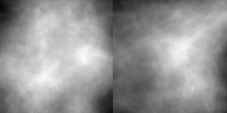
Two samples of the clustered lumpy background.

A. Positive Semidefinite Functions

To evaluate the performance of the channelized Hotelling observer, we can compute the squared SNR directly. We are not calculating sample covariance matrices but are using the numerical integral to calculate directly the elements of the covariance matrix. The natural guarantee of positivity of the estimated SNR square is lost in our method. The positive semidefiniteness of the average covariance function ensures the nonnegativity of the squared SNR. The direct Monte Carlo method cannot guarantee the positive definiteness because small deviations in the elements of the matrix usually break it. Taking a look at the covariance function expression again, we find it is important to ensure the positive semidefiniteness of the background covariance function in the numerical computation. The theory of the positive semidefinite functions and their construction is beyond the scope of this paper. A detailed discussion on this issue can be found in Refs. ¹ and ^19–21.

The covariance function of the clustered lumpy background K_b(R₁, R₂) is shift invariant since the background is stationary. In fact, we can find a real-valued symmetric function Φ(R) to construct the covariance function in the following form:

$$K_b(R_1-R_2)=\int \int {\text{d}}^{2}R\mathrm{\Phi }(R_1-R)\mathrm{\Phi }(R-R_2).$$ (4.3)

The exact expression for the function Φ (r′) is derived in Appendix C. With this function, the third term of the covariance matrix of the final image is given as

$$\begin{array}{l}{K}_{ij}^{(3)}\int \int {\text{d}}^{2}R\int \int \int \int {\text{d}}^2{r}_1^{\prime }{\text{d}}^2{R}_1\mathrm{\Phi }\\ \times \hspace{0.17em}(R_1-R)p_{\text{tot}}(r_1^{\prime },R_1)h_i(r_1^{\prime })\\ \times \hspace{0.17em}\int \int \int \int {\text{d}}^2{r}_2^{\prime }{\text{d}}^2{R}_2\mathrm{\Phi }(R_2\\ -R)p_{\text{tot}}(r_2^{\prime },\hspace{0.17em}{R}_2)h_j(r_2^{\prime }),\end{array}$$ (4.4)

where K⁽³⁾_{i j}is the ijth element of the third term of the covariance matrix. The set {∫ ∫ ∫ ∫ d²r₁′d²R₁Φ(R₁ −R) × p_tot(r₁′, R₁)h_i(r₁ ′)} composes n² ×1 column vector functions. The matrix function given by the product of the vector function and its transpose is thus a positive-definite matrix. The integral of this positive-definite matrix over its argument is the third term of the image covariance matrix and therefore is positive definite. We then perform the Monte Carlo integration over the vector function directly to get the sample function. After the above procedure, the resultant estimate of the third term is always positive definite.

B. Channel Profiles

We use the radially symmetric difference-of-Gaussian channels in this study because the signal profiles in the image are close to radially symmetric. The channel profiles are described in terms of the Fourier-transform space of the original 2D space:

$$C_j(\rho )=\text{exp}\left[-\frac{1}{2}{\left(\frac{\rho }{A{\sigma }_j}\right)}^2\right]-exp\left[-\frac{1}{2}{\left(\frac{\rho }{{\sigma }_j}\right)}^2\right],$$ (4.5)

where ρ is the radial spatial-frequency variable. The standard deviation of each channel is defined by σ_j =σ₀α^j from an initial value σ₀. The multiplicative factor A >1 defines the bandwidth of the channel. We then implement the channels in the discrete image space by using the inverse Fourier transform followed by a digitization operator D defined above. To compare the response of each channel, the channel profile is normalized so that 2π∫ dr′r′t_j(r′)² = 1, where t_j(r′) is the spatial sensitivity function calculated as the inverse Fourier transform of C_j(ρ).

5. RESULTS AND DISCUSSIONS

The clustered lumpy background has the same parameters throughout the simulation. The characteristic lengths of each blob before any random rotation are Lx = 1.5 mm and L_y =0.6 mm. The mean number of blobs per cluster is $\overline{K}$_blob = 20, and the mean number of the clusters per square centimeter is $\overline{N}$_cluster =10.17 cm⁻². The average number of blobs $\overline{K}$_blob should not be confused with the mean number of secondaries per primary $\overline{K}$ in the previous discussion. The adjustable coefficients in the blob’s exponent are α = 3.6373 mm^1/2 and β = 0.5. The standard deviation of the distribution density of the blob centers inside a cluster is σ_Φ =3.6 mm. The signal we used is a Gaussian-profile blob with the standard deviation of σ = 1.0 mm. The maximum signal level at its center is 10% of the mean background level. A unit level in the background and signal corresponds to 58.1 x-ray photons so that the exposure on the screen is comparable to the typical screen-film mammographic system with a grid that is ~9.5 mR.²²

The parameters of the fluorescent screen are primarily from the Kodak company’s mammographic screens, which use gadolinium oxysulfide activated with terbium as the phosphor. The size of the screen is 24 cm × 30 cm, and the thickness is 84 μm. The x-ray absorption coefficient is α_x =1.3 cm⁻¹. On average, each absorbed x-ray photon in the mammographic range produces 1000 visible photons that can come out of the exit surface of the screen regardless of the absorption depth. To get the Q factor in the screen model, we need the Swank factor S.²³ The value S for this screen is 0.8.²⁴ To a first approximation, the generalized BTDF can be the product between the separate spatial part and the angular part. The angular part is independent of the spatial information. We approximate the spatial distribution density of the visible photons as Gaussian with the standard deviation equal to the absorption depth. The angular distributions on all spatial positions are assumed to follow the Lambertian approximation.

The imaging lens is the part containing changing parameters. We will study the effects of these parameters on the image quality defined by the SNR of the channelized Hotelling observers. There is a folding mirror between the screen and the lens to prevent the x-ray photons from striking onto the CCD camera directly. In the simulation, the mirror is unfolded and not included in the ray-tracing routine.

The CCD camera has 128 × 128 pixels with a pixel size of 50 μm × 50 μm. The quantum efficiency is unity, and there are no gaps among adjacent pixels. This simple model of an ideal CCD camera is adequate for our simulation.

The channels used in the observer model are the dense difference-of-Gaussian channels mentioned in Abbey and Barrett’s study.⁶ This model uses ten channels. The radial frequency profile of the jth channel is the difference of the two Gaussians. The initial standard deviation in frequency is σ₀ = 0.005 pixel⁻¹, and the ratio of adjacent standard deviations is α = 1.4. The multiplicative factor defining the bandwidth of the channel is A = 1.67.

The signal position changes from an on-axis spot up to the edge of the screen. The signal position is known to the observer so that the center of the channel set is on the image of the signal center each time. When the magnification is not large enough to cover the full screen in a single CCD shot, we will move the CCD accordingly until the edge is imaged. Each time the CCD camera is shifted, the signal to be imaged will be guaranteed to be within the CCD detector and not too close to the boundary.

The first experiment is to study the effect of the aperture size of the lens. The plots of SNR versus signal position at different aperture sizes are shown in Fig. 3, and the corresponding spot diagrams at four different fields are shown in Fig. 4. The CCD camera is at the minimum rms point size position, which is commonly called the best focus position. An iris is used on the stop to control the numerical aperture of the lens. With the parameters unchanged, except for the iris diameter, the aperture size of the imaging system can be controlled. The CCD camera remains at the minimum rms spot size position as the aperture size is changed throughout this experiment. When the iris is opened up, the light throughput becomes larger so that the exposure during the same time interval becomes larger. The relatively large demagnification of the lens cuts off a large portion of the light by the relatively small numerical aperture in object space. The visible light that finally gets onto the CCD detector is so dim that it makes the Poisson noise from the x-ray photons in-significant. Instead, the lens becomes the quantum sink. Larger exposure generally improves the discrimination ability of observers because it makes the lens less of a quantum sink. Meanwhile, more aberrations are introduced into the image and make the images more blurred. The signal is gradually smeared into the background by more and more blur. Blurring effects are usually detrimental to the observer’s ability to pick a signal out of the background. The trade-off between the exposure and the blur, i.e., between the numerical aperture and the aberration, can be defined quantitatively by a certain aperture size, which makes the observer have the highest SNR.

Fig. 3.

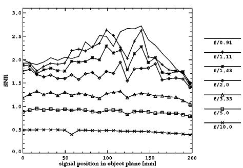
SNR plots at different aperture sizes. The signal position is measured from the optical axis on the entrance surface of the screen. The image plane position is unchanged in all cases. The aperture size is in terms of the numerical aperture in object space.

Fig. 4.

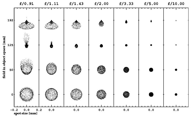
Spot diagrams at four fields of different aperture sizes. The field position is in terms of the radial distance from the optical axis on the image plane.

In this experiment, we vary the object-space numerical aperture from 0.005 up to 0.055, which corresponds to f-numbers from 10 down to 0.91. The SNR curves versus the signal position are compared in all f-number cases. From Fig. 3, the SNR increases with decreasing f-number at all fields in the f-number range from 10 to 2. The enhancement in the SNR demonstrates that the flux increase improves the observer performance at the relatively small apertures. From f-number 2 to under 1, the SNR has only limited increase at first and then is maximized at ~f/1. Although we cannot open the aperture further, we can already observe the saturation of the SNR at around f/1. In this case, decreasing the f-number further will not help in detecting signals. The maximum SNR curve numerically defines the best f-number for this lens design. This f-number quantitatively indicates the balancing point between the flux and the aberrations in the task-based manner.

At the same f-number, the aberration changes with changing field, although the exposure is almost the same within a 10° field of view in this Lambertian condition. Therefore the aberration differences are the main reason for the SNR differences at the different signal positions given any single f-number. However, from the largest f-number at 10 down to 2, each SNR curve is almost flat. From the spot diagram plots, the spot size is limited to approximately 2 × 2 pixels throughout the full range of the field of view. Therefore the observer performance is insensitive to the aberration changes when the spot width is within ~2 pixels. From f-number 2 to under 1, the SNR is not flat but has a maximum at ~ 0.7 field. From the spot diagrams, the spot size generally increases with the decreasing f-number and has a minimum at ~ 0.7 field. Most of the spots are wider than 2 pixels, which means that the observer performance is sensitive to the aberration when the spot size is beyond the 2-pixel limit. Looking at the 0.7 field in the spot diagrams, we find that the spot sizes are still around 2 pixels at different f-numbers. The trend of the SNR increasing with decreasing f-numbers is again observable at that field. Away from the 0.7 field, both aberration and exposure have visible effects on observer performance. Even though the spot size is less in the far off-axis field than in the near-axis field, the SNR is higher in the near-axis field than that far from the axis. This is because vignetting begins to reduce the exposure in the off-axis field at a low f-number, and the SNR enhancement from the smaller spot size is overcompensated by the SNR decrease from less exposure.

The second experiment is to study the effect of the working distance change of the same lens. The SNR plots at different working distances are shown in Fig. 5, and the corresponding spot diagrams are shown in Fig. 6. We choose the f/0.91 lens design from the above experiment since it yields the best observer performance. Each time we change the working distance, the lens is adjusted to the best focus position for that working distance. The closer the object is to the lens, the farther the CCD camera is from the lens and the higher the absolute magnification value. The magnification of the imaging system varies monotonically with the working distance, so we use the magnification to denote the working distance. At the designed working distance, the magnification is −0.10. This experiment examined the SNR changes at the different magnifications from −0.07 to −0.13. Because of the large demagnification used, the change in the working distance is much smaller than the distance between the screen and the lens. The observer’s performance varies considerably in spite of the small changes in the working distance.

Fig. 5.

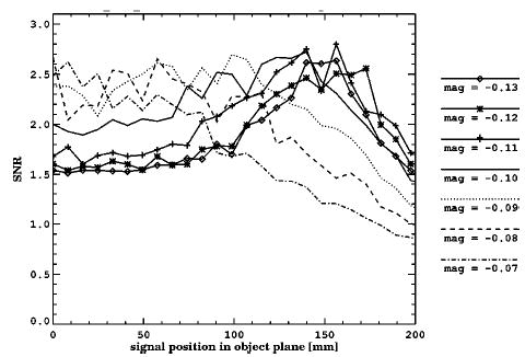
SNR plots at different working distances. The signal position is measured from the optical axis on the entrance surface of the screen. The aperture size is unchanged in all cases, with a numerical aperture of 0.055. The working distance is in terms of the magnification.

Fig. 6.

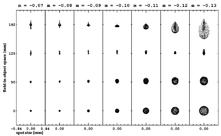
Spot diagrams at four fields of different working distances. The field position is in terms of the radial distance from the optical axis on the image plane.

The flux becomes larger when the absolute magnification is increased because the solid angle viewed from the object plane becomes larger with the increased working distance. At the close-to-axis field range, the SNR curves decrease with the increasing absolute magnifications. In this field range, the spot size quickly increases when the absolute magnification becomes larger. The SNR drop shows that the small improvement in observer performance by the flux increase cannot overcome the negative effects of blurring. At a lower absolute magnification portion, the curves are largely overlapped with an insignificant decreasing trend with increasing absolute magnifications. From the spot diagrams, the spot sizes are within the 2-pixel width limit in this portion. Therefore the observer performs similarly since the flux difference is small. When we extend to the far off-axis field region, the changing trend of the SNR curves versus the magnifications reverts, with the SNR becoming higher at the higher absolute magnification. For magnifications lower than 0.1, the SNR increases quickly when the absolute magnification becomes larger. For the cases when the absolute magnifications are higher than 0.1, the SNR curves are very close. The spot size now has a minimum at the magnification − 0.1 and increases toward both ends. Therefore the rapid improvement in observer performance below the magnification − 0.1 indicates the help from both the decreasing spot size and the increasing flux. When the absolute magnification is larger than 0.1, the detrimental effects from the increased spot size balance the positive effects from the flux, and observer performance remains the same. At ~0.7 field, the spot sizes vary little among different working distances, which makes the SNR almost unchanged.

When the absolute magnification is small, the SNR curves are relatively flat at the close-to-axis field range and generally go downward at the far off-axis field region. This is because the observer can tolerate the aberrations within 2-pixel-wide spots, which is true in the near-axis field. At the higher absolute magnification area, the effects from the aberrations become visible, and the observer performs best at ~0.7 field since the spot sizes are minimum there. Although the spot sizes are obviously different between the full field and the zero field, the observer performs similarly. This indicates that the effects of aberration should be more than just the effects of the spot size.

In this experiment, both the flux and the aberration clearly affects the observer performance. The spot size is only a coarse summary on the effect of the aberrations. More detailed effects by the aberration should not be overlooked. We can select the working distance based on the region where the signal will show up. Above all, there is only a small improvement in the near-axis fields and a larger drop in the far off-axis fields at the small absolute magnifications, and there is nearly no improvement in all fields at large absolute magnifications. We should consider the original designed working distance as the best among all choices.

The last experiment is on the focus shift of the lens. The SNR plots at different image plane positions are shown in Fig. 7, and the corresponding spot diagrams are shown in Fig. 8. On the basis of the first two experiments, we wanted to study the effect of the aberration alone. We designed the third experiment since the defocus is the most convenient way to control the blur size of the imaging lens. Also, we can check whether the best focal plane defined by the smallest rms spot size is the best in the task-based sense. In this experiment, we again use the f/0.91 lens from the first experiment. The defocus is in terms of a CCD detector plane shift from the best focal plane. The shift ranges from − 200 to 400 μm, where the negative shift means moving the CCD toward the lens, and the positive shift means moving it away. Now the fluxes in all the cases are the same. At the near-axis field region, the SNR becomes smaller when the CCD camera is moved closer to the lens. When the focus shift is between 100 and 300 μm, the SNR stays close and almost always remains at the maximum. When going out to the far off-axis field region, the SNR increases when the CCD camera is moved closer to the lens. When the shift is positive, the SNR curves overlap and remain at the upper bound. The complicated changes in SNR are related to the complex blurs by the different amounts of aberrations. From the spot diagrams, the SNR change can be explained approximately by the rms spot size, but we can also see the effect from the further details of aberrations. For the spots at the far off-axis field region and the negative focus shift, the rms spot size increases when moving closer to the lens, while the SNR is almost the same. This indicates that the tail in the spot does not affect the observer performance, even though it contributes to the rms spot size. A similar situation happens in the near-axis field region and the moderate positive focus shift; the tail around a much darker center has little effect on the SNR. On the basis of these observations, the rms spot size is not a very pertinent measure of the position of the best focus. In fact, we can see that the best focal plane should be moved a little farther away from the lens, within 100 μm from the rms best focal plane, as can be seen from the SNR curve of the 100-μm focus shift in Fig. 7.

Fig. 7.

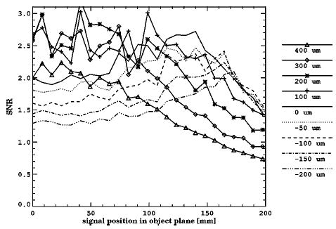
SNR plots at different image plane positions. The signal position is measured from the optical axis on the entrance surface of the screen. The aperture size is unchanged in all cases. The defocus is in terms of the distance from the ideal image plane in image space.

Fig. 8.

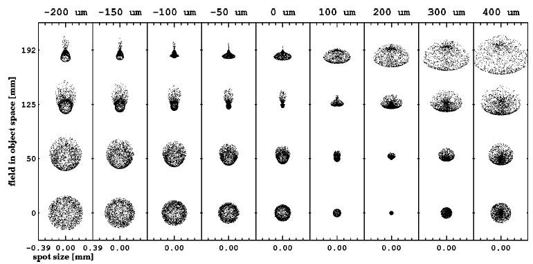
Spot diagrams at four fields of different image plane positions. The field position is in terms of the radial distance from the optical axis on the image plane.

6. CONCLUSIONS

From our simulation, the task-based lens design merit function in terms of the SNR of the channelized Hotelling observers can quantitatively take into account not only aberrations but also the flux and noise. The designers’ subjective opinion on the relationship between the aberration and other facts of the design is eliminated. The connection is instead numerically established based on statistical signal detection theory and the mathematical human vision model through the channelized Hotelling observer. We therefore call this SNR an objective or task-based design criterion. To our knowledge, this is the first time the observer’s performance has been introduced into the lens design.

We should note that the conclusions in this work, such as the best f-number at ~1.0 and the observer’s tolerance at 2-pixel-wide spots, are pertinent only to the mammographic imaging condition. Objective performance measures are critically determined by the relevant flux level and noise characteristics together with the base lens type.

APPENDIX A: MEAN IMAGE VECTOR

The discrete mean image array $\overline{g}$ is given when the operator D is applied to the continuous mean image function 〈y_g(r′)〉:

$$\begin{array}{l}\overline{g}=\langle \int {\int }_{\text{supp}}{y}_g(r^{\prime })h(r^{\prime }){\text{d}}^{\text{2}}{r}^{\prime }\rangle \\ =\int {\int }_{\text{supp}}\langle y_g(r^{\prime })\rangle h(r^{\prime }){\text{d}}^2{r}^{\prime }=D(\langle y_g(r^{\prime })\rangle ),\end{array}$$ (A1)

where h(r′) is the vector whose elements are the pixel response functions {h_i(r′)}.

The calculation of 〈y_g(r′)〉 is performed as follows:

1. Average over the displacement on the CCD detector plane {Δr′_nk}:

$$\begin{array}{l}{\langle y_g(r^{\prime })\rangle }_{\left\{\mathrm{\Delta }{r}_{nk}^{\prime }\right\}}=\sum _n\sum _k\int {\int }_{\infty }{\text{d}}^2{r}_{nk}^{\prime }{\beta }_{nk}\delta \\ \times \hspace{0.17em}(r^{\prime }-R_n-\mathrm{\Delta }{r}_{nk}-\mathrm{\Delta }{r^{\prime }}_{nk})\\ \times \hspace{0.17em}{p}_g(R_n+\mathrm{\Delta }{r}_{nk}+\mathrm{\Delta }{r^{\prime }}_{nk},\hspace{0.17em}{R}_n\\ +\hspace{0.17em}\mathrm{\Delta }{r}_{nk}|R_n,z_n)\\ =\sum _n\sum _k{\beta }_{nk}{p}_g(r^{\prime },R_n+\mathrm{\Delta }{r}_{nk}|R_n,z_n).\end{array}$$ (A2)

1. Average over {β_nk}:

$$\begin{array}{l}{\langle y_g(r^{\prime })\rangle }_{({\beta }_{nk})}=\sum _n\sum _k\langle {\beta }_{nk}\rangle p_g(r^{\prime },\hspace{0.17em}{R}_n+\mathrm{\Delta }{r}_{nk}|R_n,z_n)\\ =\sum _n\sum _k\hspace{0.17em}\text{pass}(R_n+\mathrm{\Delta }{r}_{nk},R_n|z_n)p_g(r^{\prime },\hspace{0.17em}{R}_n\\ +\hspace{0.17em}\mathrm{\Delta }{r}_{nk}|R_n,\hspace{0.17em}{z}_n).\end{array}$$ (A3)

1. Average over the displacements on the exit surface of the screen {Δr_nk}:

$$\begin{array}{l}{\langle y_g(r^{\prime })\rangle }_{(\mathrm{\Delta }{r}_{nk})}\\ =\sum _n\sum _k\int {\int }_{\infty }{\text{d}}^2{r}_{nk}\hspace{0.17em}\text{pass}(R_n+\mathrm{\Delta }{r}_{nk},\hspace{0.17em}{R}_n|z_n)\\ \times \hspace{0.17em}{p}_g(r^{\prime },\hspace{0.17em}{R}_n+\mathrm{\Delta }{r}_{nk}|R_n,\hspace{0.17em}{z}_n)\\ \times \hspace{0.17em}\overline{K_n}{(R_n,z_n)}^{-1}{p}_d(R_n+\mathrm{\Delta }{r}_{nk},\hspace{0.17em}{R}_n|z_n)\\ =\sum _n\overline{K_n}{(R_n,\hspace{0.17em}{z}_n)}^{-1}\sum _k\int {\int }_{\infty }{\text{d}}^{2}r{p}_d(r,\hspace{0.17em}{R}_n|z_n)\\ \times \hspace{0.17em}\text{pass\hspace{0.17em}}(r,\hspace{0.17em}{R}_n|z_n)p_g(r^{\prime },r|R_n,z_n)\\ =\sum _n\overline{K_n}{(R_n,\hspace{0.17em}{z}_n)}^{-1}{K}_n(R_n,z_n)\int {\int }_{\infty }{\text{d}}^{2}r{p}_d(r,\hspace{0.17em}{R}_n|z_n)\\ \times \hspace{0.17em}\text{pass\hspace{0.17em}}(r,\hspace{0.17em}{R}_n|z_n)p_g(r^{\prime },\hspace{0.17em}r|R_n,\hspace{0.17em}{z}_n).\end{array}$$ (A4)

1. Average over the gains {K_n}:

$$\begin{array}{l}{\langle y_g(r^{\prime })\rangle }_{\left\{K_n\right\}}=\sum _n\int {\int }_{\infty }{\text{d}}^{2}r{p}_d(r,\hspace{0.17em}{R}_n|z_n)\\ \times \hspace{0.17em}\text{pass\hspace{0.17em}}(r,\hspace{0.17em}{R}_n|z_n)p_g(r^{\prime },\hspace{0.17em}r|R_n,\hspace{0.17em}{z}_n).\end{array}$$ (A5)

1. Average over the absorption depth {z_n}:

$$\begin{array}{l}{\langle y_g(r^{\prime })\rangle }_{(z_n)}=\sum _n{\int }_0^d\text{d}{z}_n\frac{\text{1}}{d_x}\cdot \frac{exp(-z_n/d_x)}{1-exp(-d/d_x)}\\ \times \hspace{0.17em}\int {\int }_{\infty }{\text{d}}^{2}r{p}_d(r,\hspace{0.17em}{R}_n|z_n)\\ \times \hspace{0.17em}\text{pass\hspace{0.17em}}(r,\hspace{0.17em}{R}_n|z_n)p_g(r^{\prime },\hspace{0.17em}r|R_n,\hspace{0.17em}{z}_n).\end{array}$$ (A6)

1. Average over the absorption positions of x-ray photons {R_n}:

$$\begin{array}{l}{\langle y_g(r^{\prime })\rangle }_{(R_n)}\\ =\sum _n\int {\int }_{\text{supp}}{\text{d}}^{\text{2}}{R}_n\frac{f(R_n)}{\int \int f(R){\text{d}}^{2}R}\\ \times \hspace{0.17em}{\int }_0^d\text{d}{z}_n\frac{1}{d_x}\cdot \frac{exp(-z_n/d_x)}{1-exp(-d/d_x)}\\ \times \hspace{0.17em}\int {\int }_{\infty }{\text{d}}^{2}r{p}_d(r,\hspace{0.17em}{R}_n|z_n)\\ \times \hspace{0.17em}\text{pass\hspace{0.17em}}(r,\hspace{0.17em}{R}_n|z_n)p_g(r^{\prime },\hspace{0.17em}r|R_n,\hspace{0.17em}{z}_n)\\ =\frac{1}{d_x\overline{N}(f)}\sum _n\int {\int }_{\text{supp}}{\text{d}}^2{R}_{n}f(R_n){\int }_0^d\text{d}{z}_n\\ \times \hspace{0.17em}exp\hspace{0.17em}(-z_n/d_x)\\ \times \hspace{0.17em}\int {\int }_{\infty }{\text{d}}^{2}r{p}_d(r,\hspace{0.17em}{R}_n|z_n)\\ \times \hspace{0.17em}\text{pass\hspace{0.17em}}(r,\hspace{0.17em}{R}_n|z_n)p_g(r^{\prime },\hspace{0.17em}r|R,\hspace{0.17em}{z}_n)\\ =\frac{N(f)}{d_x\overline{N}(f)}\int {\int }_{\text{supp}}{\text{d}}^{\text{2}}Rf(R){\int }_0^d\text{d}zexp(-z/d_x)\\ \times \hspace{0.17em}\int {\int }_{\infty }{\text{d}}^{2}r{p}_d(r,\hspace{0.17em}R|z)\text{pass}(r,\hspace{0.17em}R|z)p_g(r^{\prime },\hspace{0.17em}r|R,\hspace{0.17em}z).\end{array}$$ (A7)

1. Average over the number of absorbed x-ray photons N:

$$\begin{array}{l}{\langle y_g(r^{\prime })\rangle }_N=\int {\int }_{\text{supp}}{\text{d}}^{2}Rf(R){\int }_0^d\text{d}z\frac{1}{d_x}exp(-z/d_x)\\ \times \hspace{0.17em}\int {\int }_{\infty }{\text{d}}^{2}r{p}_d(r,\hspace{0.17em}R|z)\\ \times \hspace{0.17em}\text{pass}(r,\hspace{0.17em}R|z)p_g(r^{\prime },\hspace{0.17em}r|R,\hspace{0.17em}z).\end{array}$$ (A8)

1. Average over the x-ray fluence before the entrance surface of the screen f:

$$\begin{array}{l}{\langle y_g(r^{\prime })\rangle }_N=\frac{1}{d_x}\int {\int }_{\text{supp}}{\text{d}}^{2}R\overline{f}(R){\int }_0^d\text{d}zexp(-z/d_x)\\ \times \hspace{0.17em}\int {\int }_{\infty }{\text{d}}^{2}r{p}_d(r,\hspace{0.17em}{R}_n|z)\\ \times \hspace{0.17em}\text{pass}(r,\hspace{0.17em}{R}_n|z)p_g(r^{\prime },\hspace{0.17em}r|R,\hspace{0.17em}z).\end{array}$$ (A9)

We define a conditional total PRF p_tot(r′, R|z), an overall total PRF p_tot(r′, R), and a linear operator H₁:

$$\begin{array}{l}{p}_{\text{tot}}=(r^{\prime },\hspace{0.17em}R|z)=\int {\int }_{\infty }{\text{d}}^{2}r{p}_d(r,\hspace{0.17em}R|z)\\ \times \hspace{0.17em}\text{pass}(r,\hspace{0.17em}R|z)p_g(r^{\prime },\hspace{0.17em}r|R,\hspace{0.17em}z),\end{array}$$ (A10)

$$p_{\text{tot}}(r^{\prime },\hspace{0.17em}R)=\frac{1}{d_x}{\int }_0^d\text{d}z\hspace{0.17em}exp(-d/d_x)p_{\text{tot}}(r^{\prime },\hspace{0.17em}R),$$ (A11)

$$[H_{1}f](r^{\prime })=\int {\int }_{\text{supp}}{\text{d}}^{\text{2}}R\overline{f}(R)p_{\text{tot}}(r^{\prime },\hspace{0.17em}R).$$ (A12)

The mean image array is

$$\overline{g}=[D{H}_1\overline{f}].$$ (A13)

APPENDIX B: COVARIANCE MATRIX

The covariance matrix K_g can be deduced from the autocorrelation matrix R_g and the mean image vector $\overline{g}$:

$$K_g=R_g-\langle g\rangle {\langle g\rangle }^t.$$ (B1)

With the help of the operator D, we can also obtain the autocorrelation matrix R_g out of the autocorrelation function R_g(r′₁, r′₂):

$$\begin{array}{l}{R}_g=\langle g{g}^t\rangle \\ =\langle \int \int {\text{d}}^2{r}_1^{\prime }{y}_g(r_1^{\prime })h(r_1^{\prime })\int \int {\text{d}}^2{r}_2^{\prime }{y}_g(r_2^{\prime })h^t(r_2^{\prime })\rangle \\ =\int \int \int \int {\text{d}}^2{r}_1^{\prime }{\text{d}}^2{r}_2^{\prime }h(r_1^{\prime })h^t(r_2^{\prime })\langle y_g(r_1^{\prime })y_g(r_2^{\prime })\rangle \\ =[D{R}_g(r_1^{\prime },r_2^{\prime })D^{†}].\end{array}$$ (B2)

The exact expression for the autocorrelation function is

$$\begin{array}{l}{R}_g(r_1^{\prime },r_2^{\prime })=\langle \sum _{n_1}\sum _{k_1}{\beta }_{n_1{k}_1}\delta (r_1^{\prime }-R_{n_1}-\mathrm{\Delta }{r}_{n_1{k}_1}\\ -\mathrm{\Delta }{r}_{n_1{k}_1}^{\prime })\sum _{n_2}\sum _{k_2}{\beta }_{n_2{k}_2}\delta \\ \times \hspace{0.17em}(r_2^{\prime }-R_{n_2}-\mathrm{\Delta }{r}_{n_2{k}_2}-\mathrm{\Delta }{r^{\prime }}_{n_2{k}_2})\rangle .\end{array}$$ (B3)

In the double sum over n₁ and n₂ , there are N terms with n₁ = n₂ and N² − N terms with n₁ = n₂ . For n₁ = n₂ , there are also K_n terms with k₁ = k₂and K_n² − K_n terms with k₁ ≠ k₂ . For n₁ ≠ n₂ , it is irrelevant whether k₁ = k₂ . Hence there are three cases to consider:

Case 1: n₁ = n₂ and k₁ = k₂ . The calculation parallels the derivation of the mean image array. The contribution from this part is

$${[R_g(r_1^{\prime },\hspace{0.17em}{r}_2^{\prime })]}_1=[H_{1}b](r_2^{\prime })\delta (r_1^{\prime }-r_2^{\prime }).$$ (B4)

Case 2: n₁ = n₂ and k₁ ≠ k₂ . In this case, Δr′_nk1 and Δr′_nk2 are independent, as are Δr_nk1 and Δr_nk2. The result from step (3) in Appendix A is

$$\begin{array}{l}{[R_g(r_1^{\prime },r_2^{\prime })]}_2=\sum _n\frac{K_n^2-K_n}{{\langle K_n\rangle }^2}{p}_{\text{tot}}\\ \times \hspace{0.17em}(r_1^{\prime },\hspace{0.17em}{R}_n|z_n)p_{\text{tot}}(r_2^{\prime },\hspace{0.17em}{R}_n|z_n).\end{array}$$ (B5)

Averaging over K_n in the next step requires 〈K_n(R_n , z_n)〉 and 〈K_n²(R_n , z_n)〉. Although we do not know the PDF of K_n , we can still go a little further because K_n is from the binomial selection of m(R_n , z_n), which is the total number of visible photons generated by the nth x-ray photon. The probability of a visible photon to come out of the screen is denoted by A(R_n , z_n):

$${Pr}_{K_n}(K_n)=\left[\begin{array}{c}m\\ K_n\end{array}\right]A^{K_n}{(1-A)}^{m-K_n},$$ (B6)

$$\overline{K_n}=\overline{m}A,$$ (B7)

$$\langle K_n^2|m\rangle =mA(1-A)+m^2{A}^2,$$ (B8)

$$\langle K_n^2\rangle =\overline{m}A\hspace{0.17em}(1-A)+\overline{m^2}{A}^2,$$ (B9)

$$\begin{array}{l}\text{Q(}{R}_n,\hspace{0.17em}{z}_n)\equiv \frac{\overline{K_n^2}-\overline{K_n}}{\overline{K_n{}^2}},\\ =\frac{\overline{m}A(1-A)+\overline{m^2}{A}^2-\overline{m}A}{{\overline{m}}^2{A}^2},\\ =\frac{\overline{m^2}-\overline{m}}{{\overline{m}}^2}.\end{array}$$ (B10)

With the function Q(R_n , z_n) introduced above, the result from step (4) in Appendix A is

$$\begin{array}{l}{[R_g(r_1^{\prime },\hspace{0.17em}{r}_2^{\prime })]}_2=\sum _n\frac{\overline{K_n^2}-\overline{K_n}}{\overline{K_n{}^2}}{p}_{\text{tot}}\\ \times \hspace{0.17em}(r_1^{\prime },\hspace{0.17em}{R}_n|z_n)p_{\text{tot}}(r_2^{\prime },\hspace{0.17em}{R}_n|z_n)\\ =\sum _n\text{Q(}{R}_n,\hspace{0.17em}{z}_n)p_{\text{tot}}(r_1^{\prime },\hspace{0.17em}{R}_n|z_n)p_{\text{tot}}\\ \times \hspace{0.17em}(r_2^{\prime },\hspace{0.17em}{R}_n|z_n).\end{array}$$ (B11)

The remaining steps now yield

$$\begin{array}{l}{[R_g(r_1^{\prime },r_2^{\prime })]}_2\int {\int }_{\text{supp}}{\text{d}}^{\text{2}}R\overline{f}(R){\int }_0^d\text{d}z\frac{1}{d_x}\\ \times \hspace{0.17em}exp(-z/d_x)\text{Q}(R,\hspace{0.17em}z)\\ \times \hspace{0.17em}{p}_{\text{tot}}(r_1^{\prime },\hspace{0.17em}R|z)p_{\text{tot}}(r_2^{\prime },\hspace{0.17em}R|z).\end{array}$$ (B12)

We can express this term more compactly by defining a linear operator H₂ :

$$\begin{array}{l}[H_2\overline{f}](r_1^{\prime },\hspace{0.17em}{r}_2^{\prime })=\int {\int }_{\text{supp}}{\text{d}}^{\text{2}}R\overline{f}(R){\int }_0^d\text{d}z\frac{1}{d_x}\\ \times \hspace{0.17em}exp(-z/d_x)\text{Q}(R,\hspace{0.17em}z)p_{\text{tot}}\\ \times \hspace{0.17em}(r_1^{\prime },\hspace{0.17em}R|z)p_{\text{tot}}(r_2^{\prime },\hspace{0.17em}R|z).\end{array}$$ (B13)

This part of the autocorrelation function is therefore expressed as

$${[R_g(r_1^{\prime },\hspace{0.17em}{r}_2^{\prime })]}_2=[H_2\overline{f}](r_1^{\prime },\hspace{0.17em}{r}_2^{\prime }).$$ (B14)

Case 3: n₁ ≠ n₂ . If n₁ ≠ n₂ , and considering the independence between Δr′_n1,k1 and Δr′_n2,k2, there is no correlation between R_n1 and R _n2 except possible randomness induced by f(R). For any fixed f, step (6) in Appendix A gives

$${[R_g(r_1^{\prime },\hspace{0.17em}{r}_2^{\prime })]}_3-\frac{N^2(f)-N(f)}{{\overline{N}}^2(f)}[H_{1}f](r_1^{\prime })[H_{1}f](r_2^{\prime }).$$ (B15)

Since N is a Poisson random variable at the fixed fluence f, we know that

$$\langle N^2-N|b\rangle =\text{Var(}N|f)+{\overline{N}}^2(f)-\overline{N}(f)={\overline{N}}^2(f).$$ (B16)

From step (7) of Appendix A, we have

$${[R_g(r_1{}^{\prime },\hspace{0.17em}{r}_2{}^{\prime })]}_3=[H_{1}f](r_1{}^{\prime })[H_{1}f](r_2{}^{\prime }).$$ (B17)

After step (8) in Appendix A, this case yields

$${[R_g(r_1^{\prime },\hspace{0.17em}{r}_2^{\prime })]}_3=[H_1{R}_f{H}_1^{†}](r_1^{\prime },\hspace{0.17em}{r}_2^{\prime }).$$ (B18)

By adding the Eqs. (B4), (B12), and (B18) together, we find that the autocorrelation function is

$$\begin{array}{l}{R}_g(r_1^{\prime },\hspace{0.17em}{r}_2^{\prime })=[H_1\overline{f}](r_2^{\prime })\delta (r_1^{\prime }-\hspace{0.17em}{r}_2^{\prime })+[H_2\overline{f}](r_1^{\prime },\hspace{0.17em}{r}_2^{\prime })\\ +\hspace{0.17em}[H_1{R}_f{H}_1^{†}](r_1^{\prime },\hspace{0.17em}{r}_2^{\prime }).\end{array}$$ (B18)

Because the operator H₁ is linear, the covariance function is given as

$$\begin{array}{l}{K}_g(r_1^{\prime },\hspace{0.17em}{r}_2^{\prime })=R_g(r_1^{\prime },\hspace{0.17em}{r}_2^{\prime })-\langle y_g(r_1^{\prime })\rangle \langle y_g(r_2^{\prime })\rangle \\ =[H_1\overline{f}](r_2^{\prime })\delta (r_1^{\prime }-r_2^{\prime })+[H_2\overline{f}](r_1^{\prime },r_2^{\prime })\\ +\hspace{0.17em}[H_1{K}_f{H}_1^{†}](r_1^{\prime },r_2^{\prime }).\end{array}$$ (B20)

APPENDIX C: COVARIANCE FUNCTION DECOMPOSITION

If the stationary covariance function can be decomposed into K(R) = ∫∫ d²rf(R + r)f(r)*, the Fourier transform is a positive function defined as [F₂K](ρ) = ||F(ρ)||, where F₂ is the 2D Fourier-transform operator and F(ρ) is the Fourier transform of f(R). The amplitude of the Fourier transform of the decomposition function is the square root of the Fourier transform of the covariance function.

The covariance function is¹⁸

$$\begin{array}{l}K(R_1-R_2)\\ =\frac{\overline{NK}}{A}[R_b(R_1-R_2)+\overline{K}{R}_s(R-1-R_2)],\end{array}$$ (C1)

$$\begin{array}{l}b(R,\hspace{0.17em}{R}_{\theta })=b(R,\hspace{0.17em}\phi ,\hspace{0.17em}{R}_{\theta })\\ =exp\{-\alpha R^{\beta }\\ \times \hspace{0.17em}\frac{{[L_y^2{cos}^2(\theta +\phi )+L_x^2{sin}^2(\theta +\phi )]}^{1/2}}{L_x{L}_y}\},\end{array}$$ (C2)

where b is the blob function, R_b is the autocorrelation function of the blob averaged over all the orientations,

$$\begin{array}{l}{R}_b(R_1-R_2)=\frac{1}{2\pi }{\int }_0^{2\pi }\text{d}\theta \int {\int }_A{\text{d}}^{2}Rb(R_1-R,\hspace{0.17em}{R}_{\theta })b\\ \times \hspace{0.17em}(R_2-R,\hspace{0.17em}{R}_{\theta }),\end{array}$$ (C3)

and R_s is the autocorrelation function of S_θ averaged over all the orientations, given by

$$\begin{array}{l}{R}_s=\frac{1}{2\pi }{\int }_0^{2\pi }\text{d}\theta \int {\int }_A{\text{d}}^{2}R{S}_{\theta }(R_1-R,\hspace{0.17em}{R}_{\theta })S_{\theta }\\ \times \hspace{0.17em}(R_2-R,\hspace{0.17em}{R}_{\theta }),\end{array}$$ (C4)

$$S_{\theta }(R)=\int \int {\text{d}}^2{R}^{\prime }\mathrm{\Phi }(R^{\prime })b(R-R^{\prime },\hspace{0.17em}{R}_{\theta }),$$ (C5)

where S_θ is the convolution of the cluster PDF Φ and the blob function, where the cluster PDF is the Gaussian with the standard deviation σ_φ. The constant $\overline{N}$ is the mean number of clusters within the field of view, $\overline{K}$ is the mean number of blobs per cluster, and A is the area of the field of view.

The Fourier transform of R_b results in the absolute squared Fourier transform of the blob function averaged over all the orientations:

$$[F_2{R}_b](\rho )=\frac{1}{2\pi }{\int }_0^{2\pi }\text{d}\theta \left|\right|[F_{2}b](\rho ,\theta )|{|}^2.$$ (C6)

The Fourier transform of R_s is similarly given as

$$[F_2{R}_s](\rho )=\frac{1}{2\pi }{\int }_0^{2\pi }\text{d}\theta \left|\right|[F_2{S}_{\theta }](\rho ,\theta )|{|}^2,$$ (C7)

and the Fourier transform of S_θ is the product of the Fourier transform of the blob function and the Gaussian φ:

$$[F_2{S}_{\theta }](\rho ,\theta )=exp(-2{\pi }^2{\sigma }_{\phi }^2{\rho }^2)[F_{2}b](\rho ,\hspace{0.17em}\theta ).$$ (C8)

The Fourier transform of the covariance function is given as

$$\begin{array}{l}[F_2{K}_b](\rho )=\frac{\overline{N}\overline{K}}{A}[1+\overline{K}\\ \times \hspace{0.17em}exp(-4{\pi }^2{\sigma }_{\phi }^2{\rho }^2)]\frac{1}{2\pi }{\int }_0^{2\pi }\text{d}\theta \left|\right|F_{2}b](\rho ,\theta )|{|}^2.\end{array}$$ (C9)

The amplitude of the Fourier transform of the decomposition function is the square root of that of the covariance function:

$$\begin{array}{l}|F(\rho )|={\left\{\frac{\overline{N}\overline{K}}{A}[1+\overline{K}\hspace{0.17em}exp(-4{\pi }^2{\sigma }_{\phi }^2{\rho }^2)]\right\}}^{1/2}\\ \times \hspace{0.17em}{\left[{\langle \left|\right|F_{2}b(\rho ,\theta ){\left|\right|}^2\rangle }_{\theta }\right]}^{1/2},\end{array}$$ (C10)

where 〈||F₂b(ρ, θ)||²〉_θ is the averaged absolute square of the Fourier transform of the blob function.

The Fourier transform of the blob function can be simplified as follows:

$$\begin{array}{l}[F_{2}b](\rho ,\hspace{0.17em}\theta )\\ =[F_{2}b](\rho ,\hspace{0.17em}{\phi }^{\prime },\theta )\\ ={\int }_0^{\infty }{\int }_0^{2\pi }\text{d}r\text{d}\phi rb(r,\hspace{0.17em}\phi ,\hspace{0.17em}\theta )\\ \times \hspace{0.17em}exp[-j2\pi \rho rcos({\phi }^{\prime }-\phi )]\\ ={\int }_0^{\infty }{\int }_0^{2\pi }\text{d}r\text{d}\phi r\\ \times \hspace{0.17em}exp\left\{-\alpha r^{\beta }\frac{{[L_y^2{cos}^2(\theta +\phi )+L_x^2{sin}^2(\theta +\phi )]}^{1/2}}{L_x{L}_y}\right\}\\ \times \hspace{0.17em}exp[-j2\pi \rho rcos({\phi }^{\prime }-\phi )]\\ ={\int }_0^{\infty }{\int }_0^{2\pi +\theta }\text{d}r\text{d}\phi r\\ \times \hspace{0.17em}exp\left\{-\alpha r^{\beta }\frac{{[L_y^2{cos}^2(\phi )+L_x^2{sin}^2(\phi )]}^{1/2}}{L_x{L}_y}\right\}\\ \times \hspace{0.17em}exp[-j2\pi \rho rcos({\phi }^{\prime }+\theta -\phi )].\end{array}$$ (C11)

Because the spatial function to be transformed and the Fourier-transform kernel are both periodic functions of the variable φ with 2π as one period, the integral over one period is independent of the starting point of the integration interval. The interval in Eq. (C11) can be changed into (0, 2π):

$$\begin{array}{l}[F_{2}b](\rho ,\hspace{0.17em}{\phi }^{\prime },\theta )\\ ={\int }_0^{\infty }{\int }_0^{2\pi }\text{d}r\text{d}\phi r\\ \times \hspace{0.17em}exp\left\{-\alpha r^{\beta }\frac{{[L_y^2{cos}^2(\phi )+L_x^2{sin}^2(\phi )]}^{1/2}}{L_x{L}_y}\right\}\\ \times \hspace{0.17em}exp[-j2\pi \rho rcos({\phi }^{\prime }+\theta -\phi )]\\ =[F_{2}b](\rho ,\phi +\theta ,0).\end{array}$$ (C12)

The Fourier transform of the blob function is still a periodic function of θ with a period of 2π; thus

$$\begin{array}{l}{\langle \left|\right|F_{2}b(\rho ,\hspace{0.17em}\theta ){\left|\right|}^2\rangle }_{\theta }={\langle \left|\right|F_{2}b(\rho ,\hspace{0.17em}\phi +\theta ,0){\left|\right|}^{\text{2}}\rangle }_{\theta }\\ ={\langle \left|\right|F_{2}b(\rho ,\theta ,0){\left|\right|}^{\text{2}}\rangle }_{\theta }.\end{array}$$ (C13)

The absolute square of the transform averaged over all the orientations is a radially symmetric function at last. For a radially symmetric function, the inverse Fourier transform is actually the Hankel transform, and the corresponding spatial function is a 2D real function. On the basis of this fact, the phase of the Fourier transform of the decomposition function is uniformly 0. The function can be calculated by the inverse Fourier transform of the amplitude given above:

$$\begin{array}{l}f(R)=F_2^{-1}(\{\frac{\overline{NK}}{A}[1\\ {+\overline{K}exp(-4{\pi }^2{\sigma }_{\phi }^2{\rho }^2)]\}}^{1/2}{\left[{\langle \left|\right|F_{2}b(\rho ,\hspace{0.17em}\theta ,\hspace{0.17em}0){\left|\right|}^2\rangle }_{\theta }\right]}^{1/2}).\end{array}$$ (C14)

The Fourier and inverse Fourier transform were performed for this study by the fast-Fourier-transform algorithm on a computer.

References

- 1.H. H. Barrett and K. J. Myers, Foundations of Image Science (Wiley, New York, 2004).
- 2.Rabbani M, Shaw R, Van Metter R. “Detective quantum efficiency of imaging systems with amplification and scattering mechanisms,”. J Opt Soc Am A. 1987;4:895–901. doi: 10.1364/josaa.4.000895. [DOI] [PubMed] [Google Scholar]
- 3.Cunningham IA, Westmore MS, Fenster A. “A spacial-frequency dependent quantum accounting diagram and detective quantum efficiency model of signal and noise propagation in cascaded imaging systems,”. Med Phys. 1994;21:417–427. doi: 10.1118/1.597401. [DOI] [PubMed] [Google Scholar]
- 4.B. R. Frieden, Probability, Statistical Optics, and Data Testing, 2nd ed. (Springer-Verlag, New York, 1991).
- 5.Myers KJ, Barrett HH. “Addition of a channel mechanism to the ideal-observer model,”. J Opt Soc Am A. 1987;4:2447–2457. doi: 10.1364/josaa.4.002447. [DOI] [PubMed] [Google Scholar]
- 6.Abbey CK, Barrett HH. “Human- and model-observer performance in ramp-spectrum noise: effects of regularization and object variability,”. J Opt Soc Am A. 2001;18:473–488. doi: 10.1364/josaa.18.000473. [DOI] [PMC free article] [PubMed] [Google Scholar]
- 7.N. Graham, “Complex channels, early nonlinearities, and normalization in texture segmentation,” in Computational Models of Visual Processing, M. S. Landy and J. A. Movshon, eds. (MIT Press, Cambridge, Mass., 1990), pp. 273–290.
- 8.Frishman LJ, Freeman AW, Troy JB, Schweitzer-Tong DE, Enroth-Cugell C. “Spatiotemporal frequency responses of cat retinal ganglion cells,”. J Gen Physiol. 1987;89:599–628. doi: 10.1085/jgp.89.4.599. [DOI] [PMC free article] [PubMed] [Google Scholar]
- 9.Hawken MJ, Parker AJ. “Spatial properties of neurons on the monkey striate cortex,”. Proc R Soc London, Ser B. 1987;231:251–288. doi: 10.1098/rspb.1987.0044. [DOI] [PubMed] [Google Scholar]
- 10.Webster MA, De Valois RL. “Relationship between spatial-frequency and orientation tuning of striate-cortex cells,”. J Opt Soc Am A. 1985;2:1124–1132. doi: 10.1364/josaa.2.001124. [DOI] [PubMed] [Google Scholar]
- 11.Marr D, Hildreth E. “Theory of edge detection,”. Proc R Soc London, Ser B. 1980;207:187–217. doi: 10.1098/rspb.1980.0020. [DOI] [PubMed] [Google Scholar]
- 12.Klein SA, Levi DM. “Hyperacuity thresholds of 1 sec: theoretical predictions and empirical validation,”. J Opt Soc Am A. 1985;2:1170–1190. doi: 10.1364/josaa.2.001170. [DOI] [PubMed] [Google Scholar]
- 13.Fiete RD, Barrett HH, Smith WE, Myers KJ. “The Hotelling trace criterion and its correlation with human observer performance,”. J Opt Soc Am A. 1987;4:945–953. doi: 10.1364/josaa.4.000945. [DOI] [PubMed] [Google Scholar]
- 14.E. B. Cargill, “A mathematical liver model and its application to system optimization and texture analysis,” Ph.D. dissertation (University of Arizona, Tucson, Ariz., 1989).
- 15.Eckstein MP, Whiting JS. “Lesion detection in structured noise,”. Acad Radiol. 1995;2:249–253. doi: 10.1016/s1076-6332(05)80174-6. [DOI] [PubMed] [Google Scholar]
- 16.H. H. Barrett, R. F. Wagner, and K. J. Myers, “Correlated point processes in radiological imaging,” in Physics of Medical Imaging, R. L. Van Metter and J. Beutel, eds., Proc. SPIE 3032, 110–124 (1998).
- 17.Swank RK. “Absorption and noise in x-ray phosphors,”. J Appl Phys. 1973;44:4199–4203. [Google Scholar]
- 18.Bochud FO, Abbey CK, Eckstein MP. “Statistical texture synthesis of mammographic images with clustered lumpy backgrounds,”. Opt Exp. 1999;4:33–43. doi: 10.1364/oe.4.000033. http://www.opticsexpress.org. [DOI] [PubMed] [Google Scholar]
- 19.C. Berg, J. P. Reus Christensen, and P. Russel, Harmonic Analysis on Semigroups: Theory of Positive Definite and Related Functions (Springer-Verlag, New York, 1984).
- 20.M. H. Stone, Linear Transformations in Hilbert Space and Their Applications to Analysis, Vol. 15 of the American Mathematical Society Colloquium (American Mathematical Society, New York, 1932).
- 21.Aronszajn N. “Theory of reproducing kernels,”. Trans Am Math Soc. 1950;68:337–404. [Google Scholar]
- 22.Roehrig H, Yu T, Krupinski E. “Image quality control for digital mammographic systems: initial experience and outlook,”. J Digital Imaging. 1995;8:52–66. doi: 10.1007/BF03168128. [DOI] [PubMed] [Google Scholar]
- 23.Blevis IM, Hunt DC, Rowlands JA. “X-ray imaging using amorphous selenium: detection of swank factor by pulse height spectroscopy,”. Med Phys. 1998;25:638–641. doi: 10.1118/1.598245. [DOI] [PubMed] [Google Scholar]
- 24.D. P. Trauernicht and R. Van Metter, “The measurement of conversion noise in x-ray intensifying screens,” in Medical Imaging II: Image Formation, Detection, Processing, and Interpretation, R. H. Schneider and S. J. Dwyer, eds., Proc. SPIE 914, 100–116 (1988).