Segmentation And Quantification Of Black Holes In Multiple Sclerosis

Abstract

A technique that involves minimal operator intervention was developed and implemented for identification and quantification of black holes on T1- weighted magnetic resonance images (T1 images) in multiple sclerosis (MS). Black holes were segmented on T1 images based on grayscale morphological operations. False classification of black holes was minimized by masking the segmented images with images obtained from the orthogonalization of T2-weighted and T1 images. Enhancing lesion voxels on postcontrast images were automatically identified and eliminated from being included in the black hole volume. Fuzzy connectivity was used for the delineation of black holes. The performance of this algorithm was quantitatively evaluated on 14 MS patients.

Introduction

Magnetic resonance imaging (MRI) is the most sensitive modality for visualizing multiple sclerosis (MS) lesions and provides a portal to the pathologic substrate that underlies clinical disability in MS. Several MRI measures could serve as useful surrogate markers of clinical outcome in MS clinical trials and in individual patient management. The most commonly used MR-based measures include the total lesion burden on T2-weighted images (T2 lesions), the number and volume of contrast enhanced lesions, the extent of tissue disruption as reflected by the volume of black holes on T1-weighted images (or T1 images for brevity) and magnetization transfer ratio (MTR), the magnitude of global tissue loss measured by brain and spinal cord atrophy, and the extent of neurochemical alterations based on magnetic resonance spectroscopy (MRS) (Narayana et al., 2005). A number of studies have shown that the correlation between many of these MR measures and clinical scores is weak (Sharma et al., 2004).

Of these various MR-based pathological markers, black holes have attracted considerable attention in MS. Black holes can reflect either acute edematous lesions, or matrix destruction with axonal loss as shown on post-mortem examination (Uhlenbrock and Sehlen, 1989; Van Walderveen et al., 1998). The edematous black holes initially exhibit enhancement on postcontrast MRI and often resolve with time. Black holes that represent matrix destruction and axonal loss may show better correlation with clinical disability than other MR measures. In fact Truyen et al. (1996) reported a relatively strong correlation between change in the non-enhancing black hole volumes and change in the extended disability status score (EDSS) over a period of 3 years in MS subjects.

In spite of their potential role as a surrogate in MS, there is relatively little literature on objective identification and quantification of black holes. Adams et al. (1999) have used a semiautomated region growing technique based on threshold to segment the black holes by manually selecting a seed point inside the black hole region. Molyneux et al. (2000) measured the volume of black holes using a semi-automated contour technique based on the local thresholds, which were later compared with the lesion loads obtained by outlining the boundary of the lesions on the hard copy of the image. These procedures are prone to errors, could introduce considerable operator bias, and are not practical in handling large amount of data that is typically encountered in multi-center clinical trials. In order to overcome these limitations, we have developed, implemented, and validated a method for identification and quantification of black holes with minimal human intervention.

Materials and Methods

Patients and MRI-Protocol

A total of 14 patients (10 females and 4 males; age range of 20 to 67 years with a median age of 39 years) with clinically definite MS were recruited. Their EDSS scores ranged from 1.0 to 4.0 with a median score of 2.0. Written informed consent was obtained from all patients. These studies were approved by our Institutional Committee for the Protection of Human Subjects.

Magnetic resonance images of the whole brain (from vertex to foramen magnum) were acquired on a 3T, Philips Intera scanner with a quasar gradient system (Philips Medical Systems, Best, Netherlands) using the following sequences: 1) dual fast spin echo (FSE) with TE1/TE2/TR = 9.5/90/6800 ms, 2) fluid attenuation inversion recovery (FLAIR) with TE/TR/TI = 80/10000/2600 ms, 3) pre- and post-contrast T1 weighted spin echo with TE/TR = 9.2/600 ms. Here TE, TR, and TI represent the echo, repetition and inversion times respectively. All images with these different sequences were acquired using the identical graphical prescription. The total number of images in each sequence was 44 (3 mm thick axial and contiguous) with an image matrix of 256 × 256 and a field-of-view of 240 mm × 240 mm. A SENSE factor of 2 was used for all the scans.

Identification and Quantification of Black Holes

In these studies, we are interested only in the hypointense lesions on the postcontrast T1 images. Quantification of black holes involves four major steps: 1) image preprocessing, 2) image segmentation, 3) identification of hypointense T1-lesions, and 4) identification and minimization of false classifications. These steps are described below.

Image Preprocessing

Even though all the images on a given patient are acquired in the same session with the patient's head comfortably secured, slight patient movement between different series is inevitable. Therefore, the FLAIR, pre- and post-contrast T1 images were first co-registered with the dual echo FSE images with a sub-voxel accuracy using the algorithm described elsewhere (Ashburner et al., 2000). This was followed by bias field correction (Ashburner, 2002) to compensate for the RF inhomogeneity. Extrameningeal tissues from the images were removed using a semi-automatic procedure. The stripped images were filtered using the anisotropic diffusion filter (Perona and Malik, 1990) to reduce noise without concomitant image blurring.

Segmentation of CSF, GM, WM and Hyperintense T2 Lesions

In general, there are a number of regions within the T1 images that appear hypointense that are not associated with lesions. It is essential to eliminate these regions from being falsely classified as black holes. This is realized by exploiting the fact that black holes are always associated with hyperintense lesions on T2-weighted images (T2 lesions). For an automatic association between black holes and T2 lesions, it is necessary to classify the T2 lesions.

Images were segmented into cerebrospinal fluid (CSF), gray matter (GM), white matter (WM), and lesions based on the dual echo and FLAIR images as described by Sajja et al. (2004). Briefly, following the image preprocessing, histogram normalization was performed on all the data sets so that a single feature map could be used for segmenting all the images acquired on different subjects (Narayana and Borthakur, 1995; Nyul et al., 2000). A two dimensional feature map was generated using the T2 and FLAIR images based on the Parzen window classifier (Duda et al., 2001) as described elsewhere (Bedell et al., 1997). This feature map was used to classify the whole brain into CSF, brain parenchyma, and lesions. The brain parenchyma was further segmented into GM and WM using the EM-HMRF (expectation maximization – hidden Markov random field) algorithm (Zhang et al., 2001). CSF, lesions, GM, and WM were merged together to generate the complete segmented images. The false lesion classifications were minimized using the contextual information. Finally lesions were delineated using the fuzzy-connectedness method (Udupa et al., 1997).

Identification of Black Holes

Black holes appear as regional hypointense areas on T1 images. The hypointense areas (both enhancing and non-enhancing areas) on the T1 precontrast images were identified as the regional minima on these images. A regional minimum was defined as the region of connected pixels such that any pixel in the neighborhood (six nearest neighbors along the three axes) of this region possessed an intensity that was strictly higher than the intensity of each and every pixel in the region. The identification of these regional minima was achieved by the application of grayscale morphological reconstruction by geodesic erosion (Vincent, 1993; Soille, 2003). A fixed value, say h, was added to the intensity of T1 image to generate an image, T1', in which every pixel has an intensity greater that the intensity of corresponding pixel in T1 image. The value of h was set to 3000 based on careful observation on large number of images (See “Results”). An elementary geodesic erosion of T1' denoted by ${\epsilon }_{T1}^{\left(1\right)}\left(T{1}^{\prime }\right)$, was obtained by first eroding the image with a structuring element, S, and then by taking the point-wise maximum with the image T1. Mathematically, this can be written as

$${\epsilon }_{T1}^{\left(1\right)}\left(T{1}^{\prime }\right)=\left(T{1}^{\prime }\Theta S\right)\vee T1$$ (1)

where Θ and ∨ represent the morphological erosion and point-wise maximum operators.

The grayscale morphological reconstruction of image T1' by erosion, denoted by ${\epsilon }_{T1}^{\left(n\right)}\left(T{1}^{\prime }\right)$, was realized by iteratively performing the elementary geodesic erosion until there was no further change in the reconstructed image.

In the above equation, n is the number of times the elementary erosion was applied.

The regional minima were obtained by subtracting the precontrast T1 image from the reconstructed image, and an appropriate threshold was applied to generate the binary image of the hypointense T1 lesions. Based on careful evaluation of a large number of images, this threshold was fixed and the same value was used for all the images on different subjects (see “Results”).

False positives minimization (FPM)

Black holes are always associated with T2 lesions. But the above procedure identifies all regional hypointense areas, whether or not they were associated with the T2 lesions, as black holes. These false positives were minimized by masking the binary images of regional minima with the binary maps obtained by the orthogonalization of the T2 and T1 images. Following the transformation of T1 and T2 images into one-dimensional vectors, the orthogonalization of T2 with respect to T1 was performed using

$$\overline{T2}=T2-\frac{<T2,T1>}{<T1,T1>}T1$$ (3)

where, < , > is the inner product. The orthogonalization process does not involve adjustment of any thresholds. The hypointense T1 lesions obtained after the above false positives minimization procedure were usually observed to be smaller in size compared to the black holes seen on the thresholded regional minima images. Therefore, a region growing algorithm was applied to match the sizes of the hypointense lesions.

The above procedure also classifies the enhancing voxels on the postcontrast T1 images as black holes. As these enhancing voxels appear hyperintense on the postcontrast T1 images, a preset threshold was applied to these images for differentiating the enhancing voxels from being classified as black holes. Once these enhancing voxels were identified on the postcontrast T1 images, they were eliminated from the black hole classification. As mentioned earlier, intensity normalization was applied to the T1 postcontrast images. The range of intensities on these transformed images was 0 to 4095. Since black holes on the postcontrast T1 images have lower intensities compared to the enhancing voxels, a threshold of 1500 was used to identify the enhancements after examining a large number of data sets (see “Results”). This threshold was fixed and applied to all the images acquired on all patients in this study. Since the pre- and post-contrast images were already co-registered, it is straightforward to automatically identify and eliminate enhancing voxels from being classified as black holes.

Fuzzy connectivity

In many instances, black holes do not exhibit sharp boundaries from the surrounding areas and the above procedure might not delineate the complete extent of the black holes. In these studies delineation of black holes was realized by the application of fuzzy-connectedness algorithm which is based on fuzzy adjacency and fuzzy affinity (Udupa et al., 1997). Fuzzy adjacency is the strength by which the two pixels are connected to each other spatially, and the fuzzy affinity is a measure of the strength with which the two pixels are connected to each other based on properties such as intensities of the pixels and the boundaries of objects to which the pixels belong. Fuzzy-connectedness is defined by the equation

$${\mu }_{\kappa }(x,y)={\mu }_{\alpha }(x,y)\{{\omega }_1{g}_1(x,y)+{\omega }_2{g}_2(x,y)\}$$ (4)

where, μ_α (x, y) and μ_κ (x, y) represent fuzzy adjacency and fuzzy affinity between two pixels x and y. The functions g₁ and g₂ are multivariate Gaussian functions, ω₁ and ω₂ are non-negative weights associated with these functions such that ω₁ + ω₂ = 1. Based on examination of a subset of the images, the values of ω₁ and ω₂ were set to 0.7 and 0.3, and the threshold on fuzzy affinity was set to 0.5 (see “Results”). These values were fixed and applied to all the images acquired in these studies.

Validation

The truth about the presence and extent of black holes in MS brains is not known. Therefore we relied on the expertise of an experienced neuroradiologist (RKG) in the identification and delineation of the black holes. A suite of software tools was developed to enable the neuroradiologist to identify and delineate the black holes. These tools allow the display of all the pre- and post-processed images along with the segmented images. A number of image editing tools such as paint brush and eraser were also provided in the software. The results obtained with the segmentation procedure described above were compared with the results of manual segmentation using the similarity measures (Anbeek et al., 2004) on 14 MS patients. The four similarity measures used for the validation are: 1) similarity index (SI), 2) fraction of over estimation (FOE), 3) fraction of under estimation (FUE), and 4) fraction of correct estimation (FCE). SI measures the fraction of the correctly and falsely classified black hole volumes and is perhaps the most important of all the measures. FOE and FUE measure the false positive and false negative classifications relative to the reference image, respectively, whereas FCE is the measure of the correct lesion classification relative to the reference image. These measures are formally defined as:

$$\begin{array}{cc}\hfill \mathrm{SI}& =\frac{2\times (\mathrm{Ref}\cap \mathrm{Seg})}{\mathrm{Ref}+\mathrm{Seg}}\hfill \\ \hfill & \mathrm{FOE}=\frac{\overline{\mathrm{Ref}}\cap \mathrm{Seg}}{\mathrm{Ref}}\hfill \\ \hfill & \mathrm{FUE}=\frac{\mathrm{Ref}\cap \overline{\mathrm{Seg}}}{\mathrm{Ref}}\hfill \\ \hfill & \mathrm{FCE}=\frac{\mathrm{Ref}\cap \mathrm{Seg}}{\mathrm{Ref}}\hfill \end{array}$$ (5)

In the above equations Ref and Seg denote the volumes of black holes obtained manually by the neuroradiologist and the segmentation technique, respectively.

All modules of the software were written under IDL (Interactive Data Language) and implemented on a Dell PC with a 2.2 GHz processor and 2 GB of RAM. The total computation time, excluding the image stripping which involves some operator intervention, is less than 10 minutes per subject. The typical stripping time varied between 5 to 15 minutes, depending on the experience of the individual.

Results

Segmentation

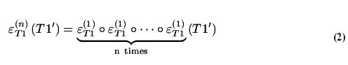
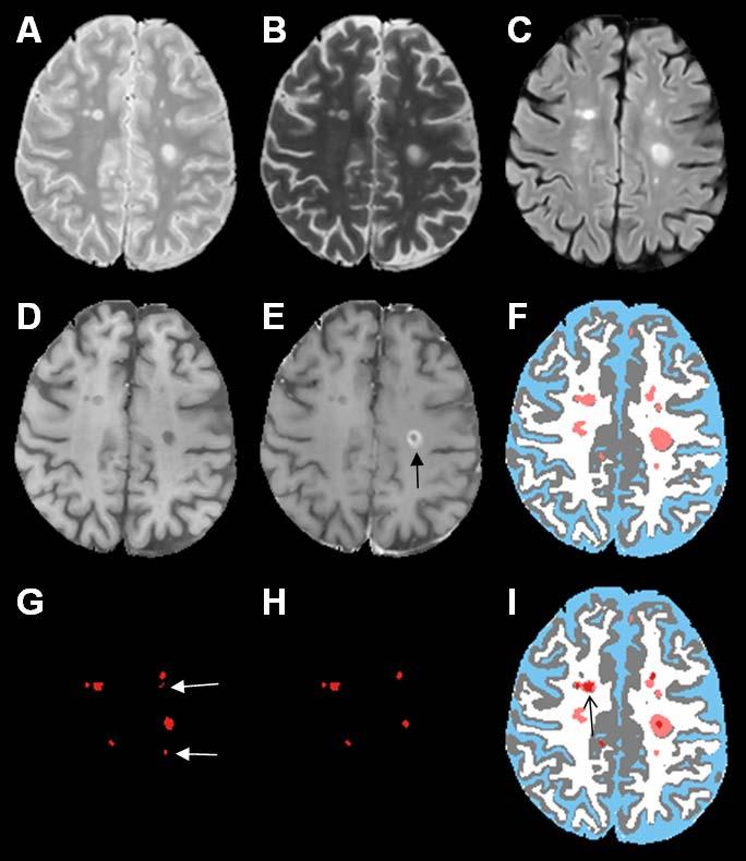
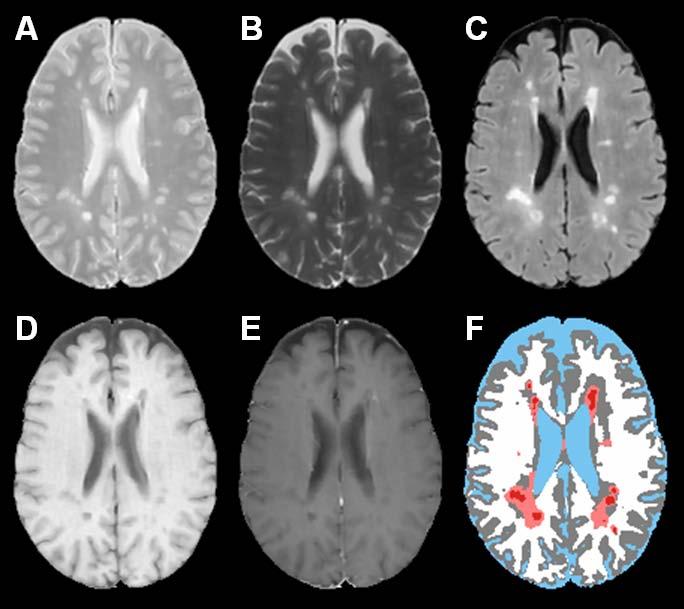
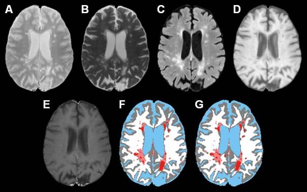
Fig. 1 shows the short echo (referred to as the proton density or PD)) (A), and long echo (T2) (B) FSE, FLAIR (C), T1 precontrast (D), T1 postcontrast (E), and the segmented (F) images using the method described by Sajja et al. (2004). The binary image with regional minima representing the hypointense T1 lesions is shown in Fig. 1G. These hypointense lesions consist of black holes, enhancing voxels, as well as lesions that are not associated with T2 lesions. The false positives seen on this image (shown by the white arrows) were minimized by masking the image by an orthogonal image of T2 and T1 and the enhancing voxels seen on the T1 postcontrast image (indicated by the black arrow on image E) were eliminated based on the intensity threshold as described earlier. The binary image of black holes following this false positives minimization procedure is shown in Fig. 1H. Following the application of fuzzy-connectedness principle, the delineated black holes along with other tissue classifications is shown in Fig. 1I. As shown in Fig. 2, the algorithm also appears to perform well even when the lesion load is relatively large. Even with all the steps taken for minimizing the false positives, in some instances, we have observed a few false positives as shown in Fig. 3. As elaborated in the “Discussion”, these false positives are the result of false T2 lesion classifications.

Fig. 1.

(A) PD, (B) T2, (C) FLAIR, (D) T1 precontrast, (E) T1 postcontrast, (F) segmented images, (CSF (blue), gray matter (gray), white matter (white), lesions (salmon)), (G) thresholded binary map of regional minima corresponding to black holes, (H) image with regional minima after false positives minimization (false positives as shown by white arrows in G were eliminated after masking G with the orthogonal image). The enhancement as shown by black arrow on image E was eliminated after differentiating enhancing lesions from black holes on T1 postcontrast image. Black holes are shown in red on final segmented image I. The effect of fuzzy delineation on the black hole is indicated by the black arrow on image I.

Fig. 2.

PD (A), T2 (B), FLAIR (C), T1 precontrast (D), T1 postcontrast (E), segmented image (F) of a subject with relatively high lesion load. The color scheme in the segmented image is CSF (blue), gray matter (gray), white matter (white), lesions (salmon), black holes (red).

Fig. 3.

PD (A), T2 (B), FLAIR (C), T1 precontrast (D), T1 postcontrast (E), segmented image (F). The color scheme in the segmented image is CSF (blue), gray matter (gray), white matter (white), lesions (salmon), black holes (red). The falsely classified black hole is shown by the arrow.

Quantitative Analysis

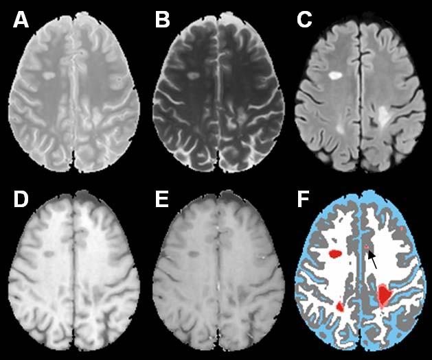
As an example, Fig. 4 shows the segmented images generated by the algorithm and the expert neuroradiologist for a visual comparison. As can be seen on this image, the automated algorithm produced both false positive and negative black holes. However, based on the comparison of a large number of images, no systematic differences were observed between the classification of the black holes by the algorithm and the neuroradiologist.

Fig. 4.

PD (A), T2 (B), FLAIR (C), T1 precontrast (D), T1 postcontrast (E), segmented image based on the algorithm (F), manually segmented image by an expert neuroradiologist (G). The color scheme in the segmented image is CSF (blue), gray matter (gray), white matter (white), lesions (salmon), black holes (red).

The identification of black holes is based on the threshold values used in the morphological grayscale reconstruction (h), identification and elimination of enhanced voxels on the postcontrast T1-images, and fuzzy connectivity (fuzzy affinity and ω₁). We varied these various thresholds to investigate their effect on the similarity measures. Changing the threshold parameter ‘h’ within the range 2200-3800 yielded identical similarity measures. Based on these results, we fixed the value of h at 3000. The threshold used for identification and elimination of contrast enhancements was varied from 1300-1600. The effect of this threshold on the similarity measures for one patient data is summarized in Table 1. The volume of black holes in this patient was determined to be 8.18 cc by the neuroradiologist. As can be seen from this table, varying the threshold between 1450 and 1600 has relatively modest effect on the similarity measures. Based on these results, we fixed the value of this threshold at 1500 which provided consistent values for all the patients. The effect of fuzzy affinity and ω₁ were also investigated. Table 2 summarizes the variation in similarity measures for black holes volumes in the same subject as in Table 1. This table indicates that both fuzzy affinity and ω₁ have only a modest effect on the similarity measures. The parameters that yielded the lowest FOE and FUE and the highest FCE are fuzzy affinity of 0.5 and ω₁ of 0.7 were chosen for all the subjects.

Table 1.

Effect of threshold for identification of enhancements on the volume of black holes and the similarity measures in one patient data.

S. No.	Threshold to eliminate enhanced voxels	Segmented volume (in cc)	FOE	FUE	FCE	SI
1.	1300	4.88	0.07	0.47	0.53	0.66
2.	1350	5.85	0.09	0.38	0.62	0.72
3.	1400	6.48	0.11	0.32	0.68	0.76
4.	1450	6.92	0.13	0.28	0.72	0.78
5.	1500	7.04	0.13	0.27	0.73	0.78
6.	1550	7.06	0.14	0.27	0.73	0.78
7.	1600	7.06	0.14	0.27	0.73	0.78

Table 2.

Effect of parameters associated with fuzzy connectivity on the volume of black holes and the similarity measures in the same subject as in Table 1.

S. No.	Threshold on Fuzzy affinity	ω1	Segmented Volume (in cc)	FOE	FUE	FCE	SI
1.	0.4	0.6	7.92	0.24	0.27	0.73	0.74
2.	0.4	0.7	7.35	0.17	0.27	0.73	0.77
3.	0.4	0.8	7.22	0.16	0.27	0.73	0.77
4.	0.5	0.4	7.23	0.18	0.30	0.70	0.74
5.	0.5	0.5	7.34	0.19	0.29	0.71	0.75
6.	0.5	0.6	7.12	0.15	0.28	0.72	0.77
7.	0.5	0.7	7.04	0.13	0.27	0.73	0.78
8.	0.5	0.8	7.00	0.14	0.28	0.72	0.77
9.	0.6	0.6	6.79	0.13	0.30	0.70	0.76
10.	0.6	0.7	6.85	0.13	0.29	0.71	0.77
11.	0.6	0.8	6.87	0.13	0.29	0.71	0.77

Table 3 summarizes the segmented volume of black holes and T2 lesion volumes on 14 subjects used for the quantitative analysis in the current studies. Quantitative analysis was performed by comparing the automatic segmentation of black holes with the results obtained by the expert neuroradiologist on the basis of the similarity measures. These similarity measures are shown in Figs. 5-8 for each of the 14 subjects for each processing step. The results of these similarity measures averaged over all the 14 subjects are summarized in Table 4. As can be seen from this table, each of the processing steps improved the agreement between the segmented and manually determined black hole volumes as indicated by the similarity index. Results shown in this table also indicate that masking with the orthogonalization of T2 images considerably reduced the false positives fraction and improved the similarity index. While the fuzzy connectivity resulted in improved the similarity index, its effect appears to be some what limited.

Table 3.

Volumes of segmented black holes and T2 lesions volumes for 14 subjects.

Subject No.	Segmented Black holes volume (in cc)	T2 lesions volume (in cc)
1	3.73	32.92
2	0.95	3.76
3	5.46	7.83
4	6.10	15.04
5	7.40	17.9
6	3.79	12.91
7	7.04	35.49
8	2.31	20.13
9	3.21	34.28
10	3.03	17.68
11	2.14	15.04
12	5.70	15.3
13	3.12	7.14
14	3.57	14.01

Fig. 5.

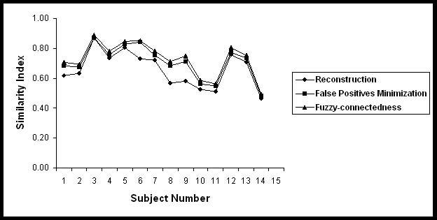
Similarity indices between the Black hole volumes obtained manually and the proposed segmentation procedure for 14 subjects at various steps of the algorithm.

Fig. 8.

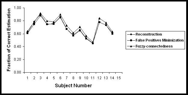
Fraction of correct estimation of Black holes in 14 subjects.

Table 4.

Values of FOE, FUE, FCE and SI between the manual and segmented black hole volumes in 14 subjects.

Steps	FOE	FUE	FCE	SI
Reconstruction	0.42 ± 0.24	0.31 ± 0.13	0.69 ± 0.13	0.66 ± 0.12
Masking	0.25 ± 0.21	0.32 ± 0.12	0.68 ± 0.12	0.71 ± 0.11
Fuzzy-connectedness	0.27 ± 0.21	0.28 ± 0.13	0.72 ± 0.13	0.73 ± 0.11

The agreement between the segmented and manual results was also evaluated using the Bland-Altman method (Bland and Altman, 1995). In the Bland Altman method, the difference between the two measurements (manual vs segmented), referred to as the bias, is plotted against the average of these two measurements, considered to be the true value. In the current studies, the difference was calculated by subtracting the black holes volumes obtained with the proposed methodology from that obtained by manual procedure. This difference was plotted against the mean of these volumes of black holes (Fig. 9). This plot shows close agreement between the two methods as indicated by the bias that lies within the two standard deviations and lack of any obvious bias.

Fig. 9.

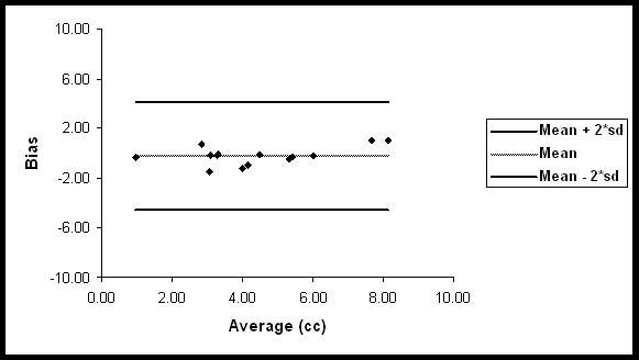
Bland-Altman plot for the comparison between manual and automatic segmentation of black holes.

Discussion

In these studies we have proposed, implemented, and quantitatively evaluated a technique for identification and quantification of black hole volumes in MS. There are number of steps involved in this method. These include stripping of images of extramenigeal tissues, image filtration, registration, bias field correction, histogram normalization, T2 lesion segmentation, identification of black holes, minimization of false black hole classification, and delineation. The only step that requires some operator intervention is the stripping the images of extrameningeal tissues. However, this procedure is significantly simplified by providing various tools such as connectivity, line editing, and island removal. Furthermore, the stripping needs to be performed only on one image set on each subject. Because all the images are coregistered, the same mask can be applied to all the images on the same subject. All the other steps are fully automated and do not require any human intervention.

Intensity or histogram normalization is an important pre-processing step in the identification of black holes. The intensity normalization used in these studies is similar to that proposed by Nyul et al. (2000). After the application of intensity normalization, the intensity range is very similar for all the PD images that are acquired on different subjects and different scanners. This is also true for the FLAIR, T2- and T1-images. Since the intensity is normalized we can use the same threshold parameters (for grayscale morphological operations, identification of enhancements, and fuzzy connectivity) for all data sets acquired on different subjects and different scanners. This is critical for automating the classification of black holes. However, intensity normalization might not work well if the acquisition parameters such as TE and TR are significantly different from scan-to-scan and result in altered relative tissue contrasts.

This method requires certain parameters for grayscale morphological operations, identification of enhancements, and fuzzy connectivity. The intensity normalization used in these studies allows us to use the same parameters for different images acquired on different subjects and different scanners.

However, since the intensities are normalized, the parameters need to be determined once. The same parameters can be applied to all the images acquired on different scanners and different subjects. More over, our analysis indicates that the values of these parameters are not critical. Our results indicate that changing these parameters by as much as 25% has relatively little effect on the final results. Thus the proposed method minimizes operator bias and is well suited for handling large amount of data that is typically acquired in multi-center clinical trials.

Our quantitative evaluation indicates a high similarity index, suggesting a close agreement between the proposed segmentation method and the manual segmentation performed by the expert neuroradiologist. The Bland-Altman analysis further indicates that our method results in minimal bias, suggesting the absence of any systematic errors in the classification of black holes. This is further confirmed by our inability to identify any systematic differences between the black hole classification by the expert neuroradiologist and the algorithm. Our studies also suggest that the algorithm works well even in those cases where the T2 lesion load is relatively high. This analysis also suggests the effectiveness of our techniques for minimizing the false classifications. It is difficult to quantitatively compare our results with other published data since few publications evaluated the performance of the segmentation using the metrics that are employed in the current studies.

A number of factors affect the accuracy with which black holes are classified using the above procedure. The proposed method relies on the accurate segmentation of T2 lesions for reducing the false black hole classification. If the T2 lesion segmentation contains false classifications, our technique could falsely classify some of the hypointense areas on T1 images as black holes. An example of such false classifications is shown in Fig. 3. Accurate image co-registration is another requirement for the satisfactory performance of the proposed method. A poor image registration technique could result in false classifications.

Partial volume averaging affects the results of image segmentation. In these studies we tried to minimize its effect by using relatively small slice thickness of 3 mm. Even in this case, the effect of partial volume averaging can be observed in the segmentation of GM and WM in some regions at the interface of brain and CSF (Fig. 1).

As indicated earlier, the false positives minimization step slightly reduces the size of the black holes. It is possible that this step might eliminate very small black holes, particularly subtle ones.

Currently, the proposed methodology is used for determining the black hole volumes in a number of ongoing multi center clinical trials in MS.

In this paper, we presented a method for the identification and quantification of “black holes” in MS. This method involves minimal human intervention and is well suited for handling large number of data sets. Quantitative analysis indicates excellent agreement between the results obtained with this method and the manual segmentation performed by an expert neuroradiologist.

Fig. 6.

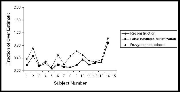
Fraction of over estimation of Black holes in 14 subjects.

Fig. 7.

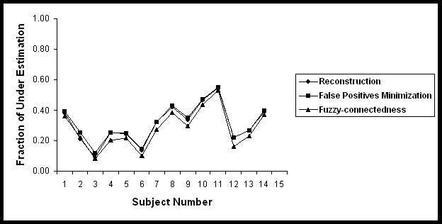
Fraction of under estimation of Black holes in 14 subjects.

References

- Adams H-P, Wagner S, Sobel SF, Slivka LS, Sipe JC, Romine JS, Beutler E, Koziol JA. Hypointense and hyperintense lesions on magnetic resonance imaging in secondary-progressive MS patients. European Neurology. 1999;42:52–63. doi: 10.1159/000008069. [DOI] [PubMed] [Google Scholar]
- Anbeek P, Vincken KL, van Osch MJP, Bisschops RHC, van der Grond J. Probabilistic segmentation of white matter lesions in MR imaging. NeuroImage. 2004;21:1037–1044. doi: 10.1016/j.neuroimage.2003.10.012. [DOI] [PubMed] [Google Scholar]
- Ashburner J. Another MRI bias correction approach; 8th International Conference on Functional Mapping of the Human Brain; Japan. 25-28 September.2002. [Google Scholar]
- Ashburner J, Andersson J, Friston KJ. Image registration using a symmetric prior--in three-dimensions. Human Brain Mapping. 2000;9:212–225. doi: 10.1002/(SICI)1097-0193(200004)9:4<212::AID-HBM3>3.0.CO;2-#. [DOI] [PMC free article] [PubMed] [Google Scholar]
- Bedell BJ, Narayana PA, Wolinsky JS. A dual approach for minimizing false lesion classifications on magnetic resonance images. Magn Reson Med. 1997;37:94–102. doi: 10.1002/mrm.1910370114. [DOI] [PubMed] [Google Scholar]
- Bland JM, Altman DG. Comparing methods of measurement: why plotting difference against standard method is misleading. Lancet. 1995;346:1085–1087. doi: 10.1016/s0140-6736(95)91748-9. [DOI] [PubMed] [Google Scholar]
- Duda RO, Hart PE, Stork DG. Pattern Classification. 2nd John Wiley and Sons; New York: 2001. [Google Scholar]
- Molyneux PD, Brex PA, Fogg C, Lewis S, Middleditch C, Barkhof F, Sormani MP, Filippi M, Miller DH. The precision of T1 hypointense lesion volume quantification in multiple sclerosis treatment trials: a multicenter study. Multiple Sclerosis. 2000;6:237–240. doi: 10.1177/135245850000600405. [DOI] [PubMed] [Google Scholar]
- Narayana PA, Borthakur A. Effect of radio frequency inhomogeneity correction on the reproducibility of intra-cranial volumes using MR image data. Magn Reson Med. 1995;33:396–400. doi: 10.1002/mrm.1910330312. [DOI] [PubMed] [Google Scholar]
- Narayana PA, Mehta M, Wolinsky J. Magnetic resonance in multiple sclerosis. In: Jagannathan NR, editor. Recent advances in MR Imaging and Spectroscopy. Jaypee Brothers Medical Publishers Ltd; New Delhi: 2005. pp. 154–185. [Google Scholar]
- Nyul LG, Udupa JK, Zhang X. New variants of a method of MRI scale standardization. IEEE Trans Med Imag. 2000;19:143–150. doi: 10.1109/42.836373. [DOI] [PubMed] [Google Scholar]
- Perona P, Malik J. Scale-space and edge detection using anisotropic diffusion. IEEE Trans Pattern Anal Mach Intell. 1990;12:629–639. [Google Scholar]
- Sajja BR, Datta S, He R, Narayana PA. A unified approach for MS lesion segmentation on MR images. Proc of IEEE Engg Med Bio Soc (EMBS) 2004:1778–1781. doi: 10.1109/IEMBS.2004.1403532. [DOI] [PubMed] [Google Scholar]
- Sharma J, Sanfilipo MP, Benedict RHB, Weinstock-Guttman B, Munschauer FE, II, Bakshi R. Whole-brain atrophy in multiple sclerosis measured by automated versus semiautomated MR imaging segmentation. AJNR Am J Neuroradiol. 2004;25:985–996. [PMC free article] [PubMed] [Google Scholar]
- Soille P. Morphological Image Analysis. Springer-Verlag; New York: 2003. [Google Scholar]
- Truyen L, van Waesberghe JH, van Walderveen MA, van Oosten BW, Polman CH, Hommes OR, Ader HJ, Barkhof F. Accumulation of hypointense lesions (“black holes”) on T1 spin-echo MRI correlates with disease progression in multiple sclerosis. Neurology. 1996;47:1469–1476. doi: 10.1212/wnl.47.6.1469. [DOI] [PubMed] [Google Scholar]
- Udupa JK, Wei L, Samarasekera S, Miki Y, van Buchem MA, Grossman RI. Multiple sclerosis lesion quantification using fuzzy-connectedness principles. IEEE Trans Med Imag. 1997;16:598–609. doi: 10.1109/42.640750. [DOI] [PubMed] [Google Scholar]
- Uhlenbrock D, Sehlen S. The value of T1-weighted images in the differentiation between MS, white matter lesions, and subcortical arteriosclerotic encephalopathy (SAE) Neuroradiology. 1989;31:203–212. doi: 10.1007/BF00344344. [DOI] [PubMed] [Google Scholar]
- Van Walderveen MA, Kamphorst W, Scheltens P, van Waesberghe JH, Ravid R, Valk J, Polman CH, Barkhof F. Histopathologic correlate of hypointense lesions on T1-weighted spin-echo MRI in multiple sclerosis. Neurology. 1998;50:1282–1288. doi: 10.1212/wnl.50.5.1282. [DOI] [PubMed] [Google Scholar]
- Vincent L. Morphological grayscale reconstruction in image analysis: applications and efficient algorithms. IEEE Trans Image Proc. 1993;2:176–201. doi: 10.1109/83.217222. [DOI] [PubMed] [Google Scholar]
- Zhang Y, Brady M, Smith S. Segmentation of brain MR images through a hidden Markov random field model and the expectation-maximization. IEEE Trans Med Imag. 2001;20:45–57. doi: 10.1109/42.906424. [DOI] [PubMed] [Google Scholar]