Measuring V1 Receptive Fields Despite Eye Movements in Awake Monkeys

Abstract

One difficulty with measuring receptive fields in the awake monkey is that even well-trained animals make small eye movements during fixation. These complicate the measurement of receptive fields by blurring out the region where a response is observed, causing underestimates of the ability of individual neurons to signal changes in stimulus position. In simple cells, this blurring may severely disrupt estimates of receptive field structure. An accurate measurement of eye movements would allow correction of this blurring. Scleral search coils have been used to provide such measurements, although little is known about their accuracy. We have devised a range of approaches to address this issue: implanting two coils into a single eye, exploiting the small size of V1 receptive fields and developing maximum-likelihood fitting techniques to extract receptive field parameters in the presence of eye movements. All our investigations lead to the same conclusion: our scleral search coils (which were not sutured to the globe) are subject to an error of approximately the same magnitude as the small eye movements which occur during fixation: SD ~ 0.1°. This error is large enough to explain the SD of measured vergence in the absence of any real changes in vergence state. This, and a variety of other arguments, indicate that the real variation in vergence is much smaller than coil measurements suggest. These results suggest that monkeys, like humans, maintain very stable vergence. The error has a slower time course than fixational eye movements so that search coils report the difference in eye position between two consecutive trials more accurately than the eye position itself on either trial. Receptive field estimates are unlikely to be improved by assuming the coil record is veridical and correcting for eye position accordingly. However, receptive field parameters can reliably be determined by a fitting technique that allows for eye movements. It is possible that suturing coils to the globe reduces the artifacts, but no method has been available to demonstrate this. These receptive field measurements provide a general means by which the reliability of eye-position measurements can be assessed.

INTRODUCTION

One of the most striking characteristics of visual cortical neurons is that they are activated only by stimuli presented in a restricted region of space, the receptive field (RF). When the eyes move, an RF that has a fixed retinal location will change its location in external space. In the primary visual cortex of awake monkeys, careful examination of neuronal responses and eye-position records has shown that the RF is indeed fixed in retinal coordinates, even after small fixational eye movements (Gur and Snodderly 1997; Gur et al. 1997).

This raises a potentially serious problem for the study of receptive fields in awake animals. Even animals with extensive training on a fixation task make small eye movements during fixation, so that there is a variable relationship between the external stimulus location and the retinal stimulus location. Of course, the extent to which this disrupts RF measures will depend on the relative size of the eye movements and the RF. In monkey striate cortex, many RFs are sufficiently small that fixational eye movements pose a substantial problem. The structure of the RF may be blurred, and its size is likely to be overestimated. While for many applications an overestimate of RF size may be a relatively benign error, it nevertheless means that the sensitivity of V1 cannot be accurately assessed. Blurring of the RF by eye movements will result in an underestimate of the ability of individual neurons to discriminate changes in stimulus position.

This problem is most commonly ignored in the hope that the animals’ fixation is sufficiently precise that measures of RF size or structure are not in fact disrupted. More recently, several studies have used measures of eye position to correct for movements and estimate the retinal location of each stimulus, either with scleral search coils (Conway 2001; Livingstone 1998; Livingstone and Tsao 1999) or a double Purkinje image eye tracker (Gur and Snodderly 1987, 1997; Gur et al. 1997; Kagan et al. 2002; Snodderly and Gur 1995).

Gur, Snodderly, and colleagues have used the Purkinje eye tracker to stabilize images on-line (that is, they add the recorded eye position to the stimulus position to keep the retinal position constant) (Gur and Snodderly 1987; Gur et al. 1997; Kagan et al. 2002; Snodderly and Gur 1995). These studies show convincingly that adjusting the image position with the measured eye position is superior to making no adjustment. This is the clearest evidence available that V1 receptive fields are fixed in retinal coordinates. However, these data do not rule out any artifact in the eye-position measures. This would require a quantitative comparison between measured eye-position variation and RF size, both with and without correction. Furthermore, the data demonstrating the effectiveness of stabilization were all collected over short time periods. These have been used with care by these authors to establish the relevant scientific points, but the long-term stability of the eye-position measures remains unproven.

In contrast, other authors (Conway 2001; Livingstone 1998; Livingstone and Tsao 1999) have used scleral search coils to correct for eye movements over extended recording sessions (hours). Clearly, such an approach places heavy reliance on the long-term accuracy of eye-position recording. The scleral search coil yields very precise measures. However, the very small high-frequency noise does not guarantee accuracy—it is quite possible that there are instrumental errors that change slowly enough not to compromise the precision. Any adjustment of the instrument’s offset during an experiment would tend to conceal any such drift. We are unaware of any study that has assessed the absolute accuracy of eye-position recordings with the scleral search coil.

That scleral search coil signals contain significant inaccuracies is not merely a logical possibility. When recording the position of both eyes with scleral search coils, we have often noticed slow drifts in recorded vergence angle, and others have noted the same phenomenon (F. Miles, personal communications). Thus the raw data appear to show that the subjects are maintaining a stable misconvergence, which seems unlikely given that a variety of methods suggest that fixation disparities in humans are small and show very little variation (SDs < 2 min arc) (Collewijn et al. 1988; Duwaer 1983; Enright 1991; Jaschinski-Kruza and Schubert-Alshuth 1992; Ogle 1964; Riggs and Neill 1960; St Cyr and Fender 1969).

Because these observations are anecdotal, we attempt here to examine the reliability of these measures, exploiting the small RFs of V1 receptive fields. In one animal, we also implanted two coils in one eye. All of these measures suggested that there are substantial errors in the estimation of eye position from scleral search coils. This led us to develop a method for measuring RF size that does not depend on information about absolute eye position.

METHODS

Two adult male macaque monkeys were implanted under general anesthesia with scleral search coils in both eyes, a head-restraining post, and a recording chamber placed over the operculum of V1. The coil surgery closely followed the description in Judge et al. (1980); in particular, the coil was not sutured to the sclera, and a strain-relief pouch was created. The monkeys were trained to maintain fixation on a small white dot for fluid reward. If fixation was maintained to within ± 1° of the dot for 2 s, a reward was delivered. This relatively large window was chosen so as not to suppress small eye movements during fixation. Coil offsets were set at the beginning of each experiment and not adjusted thereafter. All protocols were approved by the Institute Animal Care and Use Committee and complied with Public Health Service policy on the humane care and use of laboratory animals.

Glass-coated platinum-iridium electrodes (Frederick Haer) were introduced transdurally into the operculum of striate cortex. Electrode position was controlled with a custom-made microdrive that used an ultra-light stepper motor mounted directly onto the recording chamber. The signal was amplified (Bak Electronics), band-pass filtered (100 Hz to 10 kHz), digitized at 32 kHz and stored to disk on a PC running the Datawave Discovery package. Single-unit isolation was always checked off-line. The vertical and horizontal positions of both eyes were sampled at 5.3 kHz and then averaged in groups of eight consecutive samples to give a sampling rate of 660 Hz.

Stimuli were generated on a Silicon Graphics Octane workstation and presented on two Eizo Flexscan F980 monochrome monitors (mean luminance: 41.1 cd/m², contrast: 99%, frame rate: 72 Hz) via a Wheatstone stereoscope. That is, the monitors were placed on either side of the monkey, who viewed the images via mirrors placed at an angle of 45° 2 cm in front of each eye. At the viewing distance used (89 cm) each pixel in the 1,280 × 1,024 display subtended 1.1 min arc. Within each 2-s fixation period, four stimuli were presented, each lasting 415 ms with an inter-stimulus interval of ≥100 ms.

Receptive fields were mapped with sinusoidal luminance gratings. Initially, a circular patch of grating was manipulated manually to determine approximately the preferred orientation and spatial frequency and the boundaries of the minimum response field. Quantitative measurement of orientation preference used circular grating patches (≥9 different orientations spanning 180°), quantitative estimation of spatial and temporal frequency tuning used larger rectangular grating patches. Quantitative estimation of RF width and location then used a narrow strip of grating at the preferred orientation, whose location varied from trial to trial along an axis orthogonal to the preferred orientation. In many cases, the width of the strip was smaller that the spatial period of the grating, so the stimulus was similar to a stationary bar with a sinusoidal variation in luminance over time. The temporal frequency was usually 4 Hz, but in a few neurons (12), higher frequencies were necessary to elicit a brisk response. The strip was substantially longer than the minimum response field (MRF; mean length, 5°), so that only variation in stimulus and eye position along one axis influenced the stimulus within the MRF. Monocular stimuli, presented to the dominant eye, were used, although the fixation marker was always visible in both eyes. To be included in the study, neurons had to respond with at least three spikes to a 415-ms presentation at the optimal position (as an average over ≥3 repetitions of the stimulus), and the mean number of repetitions at each stimulus position had to exceed 3. Fifty-seven neurons satisfied these criteria, including six pairs recorded simultaneously.

In addition to eye movements, any blinks that occurred during the presentation of a stimulus could be a source of error. All trials which included any part of a blink were discarded. Both blinks and micro-saccades were detected by differentiating the conjugate eye-position signals, ḣ ḣ and v̇ being the magnitude of the horizontal and vertical velocities, respectively. Whenever the speed of conjugate movement (√ḣ² + v̇²) exceeded 10°/s, an event was deemed to have started. Two characteristics distinguished blinks from true saccades. First, the displacement was transient so that the excursion during the event was large relative to the size of any net displacement. Second, the transient displacements occurred at slightly different times in the two eyes, giving rise to an apparent transient vergence movement (with both vertical and horizontal vergence changes). The latter was sufficiently distinctive to allow reliable blink detection. If an event identified by a conjugate eye velocity >10°/s was also associated with a vergence velocity (vertical or horizontal) that exceeded 5°/s for ≥100 ms, it was invariably a blink. To confirm this, calibration data were gathered by viewing the pupil with an infrared sensitive CCTV camera. A photodiode was placed over the video image of the pupil, and its output low-pass filtered at 30 Hz. Reflections from the lids then produced a readily detectable change in this output when a blink occurred. A total of 2,072 saccades (mostly microsaccades) and 162 blinks were recorded. No saccades were misclassified as blinks, and all 162 blinks were correctly identified.

The variation in spike count as a function of stimulus location was fit with a Gaussian, first by a simple least-squares fit and later by a more sophisticated maximum-likelihood approach. It is inappropriate to use least-squares fitting on neuronal spike counts directly because their variance is proportional to the mean (Dean 1981). However, at least for large firing rates, this implies that the square-root of the spike count has approximately constant variance. We therefore fit the square-root of a Gaussian to the square-root of spike counts (Prince et al. 2002b). We compared the effect of ignoring eye movements, and of correcting for eye movements using the scleral search coil. We also developed a novel fitting method designed to enable an accurate reconstruction of receptive field parameters even in the presence of eye movements and inaccurate coil measurements (see APPENDIX). It is based on the observation that the artifact affecting the coil is of lower frequency than the signal and hence that the coil accurately reports changes in eye position between two consecutive trials even if it is unreliable over long periods of time. Knowing the difference in eye position between two trials, as well as the spike counts recorded on each trial, provides important additional constraints on the eye position and RF parameters. All analysis code was written in MATLAB 6.1 (The Mathworks), and the fitting employed the routine FMIN-SEARCH from MATLAB’s optimization toolbox.

RESULTS

Binocular measures

In a separate study of disparity-selective neurons, selectivity for disparity in random dot stereograms (RDS) was measured. In several instances, the tuning curve was measured in two separate blocks separated by several minutes.

Figure 1 shows two examples (1 for each monkey) in which the recorded vergence angle changed substantially in the period between the two blocks, yet it is clear that there has been no such displacement of the tuning curves. This implies either that there has not in fact been a change in vergence angle or that the neuronal responses somehow compensate for such changes. The latter interpretation seems very unlikely because when vergence is explicitly manipulated disparity tuning curves are displaced accordingly (Cumming and Parker 1999). Two other approaches were used to distinguish these possibilities.

FIG. 1.

Disparity selectivity for random dot patterns, measured in 2 independent blocks separated in time (by 6.61 min for duf190 and 5.93 min minutes for ruf102). The mean ver-gence angle was calculated in each block (legend). Vergence angle is expressed relative to the correct angle for the fixation dot (i.e., it is fixation disparity). Despite the change in ver-gence, there is clearly no corresponding shift in the tuning curve.

Comparing search coils in the same eye

First, in monkey Duf, a third coil was implanted so that there were two coils in the right eye. (This was done because the drifts in that eye seemed larger than usual, so it was necessary to implant a new coil for other reasons.) The eye-position readings of all three coils were measured simultaneously for a series of 6,284 415-ms stimulus presentations similar to those used in recording experiments. Trials where the monkey blinked or made a saccade were removed, leaving 3,121 trials. The mean horizontal position ( $\overline{\text{L}},\mathrm{\hspace{0.17em} }\overline{\text{R}1},\mathrm{\hspace{0.17em} }\overline{\text{R}2}$) was calculated for each 415-ms stimulus presentation. The SD was then calculated for the three possible “vergence” measures: $\text{SD}(\overline{\text{L}}-\overline{\text{R}1})=0.202°,\mathrm{\hspace{0.17em} }\text{SD}(\overline{\text{L}}-\overline{\text{R}2})=0.088°$, and $\text{SD}(\overline{\text{R}1}-\overline{\text{R}2})=0.157°$. The difference between two coils in the same eye shows substantial variation (0.157°), establishing beyond doubt that eye-position measures with scleral search coils can contain significant inaccuracies.

One might argue that some mechanical interaction between the two coils in one eye induced inaccuracies that were not present when only one coil was implanted. If this was the case, then the measures of $\overline{\text{L}}-\overline{\text{R}1}$ taken before the second coil was implanted should show a smaller SD of vergence. In fact, the SD of vergence prior to implanting the second coil was slightly larger (mean SD across 28 experiments was 0.216°) than the equivalent measure on the same two coils subsequently.

Coil R1 was replaced because of its unusually large drifts. Vergence measured with this coil has a larger SD (0.202°) than with the newer coil (0.088°). Thus a possible interpretation is that coils L and R2 are veridical, while R1 is subject to a large artifact. Under this interpretation, (L – R2) represents the monkey’s vergence state, (R1 – R2) represents the error on coil R1 (SD ~ 0.16), and (L – R1) represents vergence plus the error on R1. Because the real changes in vergence should have a different structure than artifactual drifts, examining the time course of the three “vergence” measures should reveal these differences. We therefore examined the Fourier amplitude spectra of all three measures. Of course, the animal may make saccades during inter-trial intervals, which may add a common signal to all three. To prevent this, our analysis uses only data recorded during fixation trials. To look at low frequencies, we first divided the ~3,000 trials into 10 groups of 300 roughly consecutive trials, and plotted mean vergence angle ( $\overline{\text{L}}-\overline{\text{R}1},\mathrm{\hspace{0.17em} }\overline{\text{L}}-\overline{\text{R2}},\mathrm{\hspace{0.17em} }\overline{\text{R}1}-\overline{\text{R}2}$, averaged over 1 trial) over the 300 trials. For each group of 300 trials, we calculated the Fourier spectrum of this between-trials vergence variation, normalized to unit power. Figure 2A shows the average value of this spectrum, averaged over the 10 groups. The spectra of the three vergence measures are remarkably similar. To look at high frequencies, we looked at fluctuations within each 415-ms trial (L – R1, L – R2, R1 – R2). Figure 2B shows the Fourier spectrum of these instantaneous vergences, averaged over all 3,121 trials. The three spectra are indistinguishable.

FIG. 2.

Fourier amplitude spectra of normalized “vergence” measures from different coils (left – right 1, left – right 2, right 1 – right 2). A is based on records of the mean vergence (averaged over each 415-ms trial) over 300 trials. It shows the average Fourier amplitude spectrum of these records, averaged over 10 groups of 300 trials. Irrespective of which 2 coils are used to obtain the “vergence” measure, the spectrum has the same shape. B: amplitude spectrum of vergence records over a single 415-ms stimulus presentation, sampled at 660 Hz; the plot shows the mean amplitude spectrum averaged over 3,121 presentations. In both A and B, the heavy solid line shows the results of a simulation, in which the coil record in each eye was modeled as a random walk. At each 1.5 ms time step, each simulated coil record was, independently, either incremented or decremented 1 unit. The probability of increment at a given timestep was set to be ½ erfc(x/2n²), where erfc is the complementary error function, x the current distance from the origin, and n was set to be 30 units. For a sufficiently long walk, the distribution of all the x values visited during the walk is approximately normal with SD = n. The simulation was repeated 100 times with different random walks; the plots show the mean results (which is why they are smoother than the experimental data). All spectra have been normalized to contain the same total power.

If coils L and R2 are assumed to be veridical, this means that the error on coil R1 just happens to have exactly the same frequency profile as the animal’s vergence movements. This seems an improbable coincidence. We suggest, rather, that our monkeys, like human subjects, have vergence errors close to zero and that the “vergence” measure obtained from the coils is dominated by artifacts on the coil signals. Under this interpretation, the errors on the coils have different magnitude (coil R1 is subject to a larger error than R2), but the Fourier spectra are similar because they all reflect the same underlying process.

In fact, the Fourier spectra at high frequencies are strikingly close to that of a simple one-dimensional random walk, whose value is either incremented or decremented at every time step, with equal probability. This random walk has too much power at lower frequencies, but simply by making the probability of stepping back toward the origin increase with distance from the origin, (see legend to Fig. 2) a much better match is obtained. This rough model provides a surprisingly good match to the experimental Fourier spectra over frequencies from 330 Hz down to 0.008 Hz. At frequencies < 0.008 Hz, the Fourier spectrum of the experimental vergence measures has more power than the model, continuing to rise down to the lowest frequencies measured (~0.0008 Hz, not shown). It is nonetheless striking that such a simple model explains the observed Fourier spectra over a very wide frequency range. Importantly, the same deviations from the model are seen in all three coil difference signals. The failure of the simple model at very low frequencies in no way undermines the conclusion that all three difference signals are generated by a similar process. This in turn suggests that none of them has much power that reflects real changes in vergence, which implies that real vergence changes are small relative to the size of the artifact.

Analysis of variability

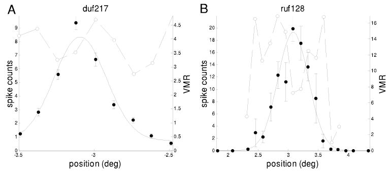
The second approach exploited the variability of neuronal spike counts. If there are real changes in vergence during the fixation task, then this should influence the firing rate of disparity-selective neurons. However, this will only be the case for stimulus disparities at which the neuron is sensitive to small changes. During presentation of an uncorrelated dynamic RDS, change in vergence angle should have no effect. Similarly, at the flanks of the disparity tuning curve, where small changes in disparity have no effect on activity, the variability in firing rate will not be influenced by vergence fluctuations. Figure 3 shows the relationship between disparity tuning and spike count variability (the variance:mean ratio, VMR) for two narrowly tuned neurons. It is clear that the variability is highest where the rate of change of spike count with respect to disparity is greatest. This indicates that there are changes in vergence, and the neuronal activity is determined by the resultant disparity changes. It is possible to use data like these to estimate the variability of vergence, if one assumes that the ratio (spike count variance)/(spike count mean), measured across repeated presentations of the same stimulus, is a constant for each neuron. This constant, k, can be estimated from the VMR for those points on the tuning curve that are insensitive to disparity changes (we used a slope of < 10 spikes/s per degree of disparity). At each disparity, the total variance of the count, σ_c², is approximated by the sum of a term related to the mean firing rate, and a term caused by vergence fluctuations (with an SD σ_v)

FIG. 3.

Variability in spike count induced by fluctuations in vergence angle. At disparities where the neuronal response rate changes rapidly as a function of disparity, even small fluctuations in vergence will increase spike count variability. ○ and —, the disparity tuning of 2 neurons (firing rate plotted on the left axis). • and - - -, the variance:mean ratio (VMR) of the spike count distributions (scale on the right axis). It is clear that this ratio is high at disparities where the slope is high, exactly as expected if the spike count depends only on the absolute retinal disparity of the stimulus and there is some fluctuation in vergence. Note that very high VMRs are observed here because the neurons are very sensitive to disparity. Only very small vergence fluctuations are required to produce these high VMRs (an SD of 0.012° is sufficient for duf069, 0.011° for ruf066).

$${\sigma }_c^2=k.\text{mean}+{\sigma }_v^2{\text{slope}}^2$$ (1)

where slope is the rate of change of the spike count with respect to disparity, and mean the mean firing rate at that point. To estimate the value of slope, a Gabor function was fitted to each disparity tuning curve, and the slope of the fit at each point was used. The resulting estimate of σ_v is clearly most reliable when slope is high. Indeed, when the slope is low enough that σ_v ²slope² becomes small relative to k.mean, sampling variation can give rise to points where σ_c ² < k.mean, in which case the vergence SD cannot be estimated.

Restricting this analysis to data points associated with a high rate of change of firing rate with respect to disparity therefore yields the most reliable estimates of σ_v, but limits the size of the dataset. If only slopes > 400 spikes · s⁻¹ ·° ⁻¹ of disparity are included in the analysis, then 6/114 disparity tuned neurons yielded an estimate of σ_v. For each neuron, σ_v was estimated at each point exceeding this slope, and the mean σ_v calculated. The mean of these across the 6 neurons was 0.0111°, and they were in close agreement with one another, with an SD of only 0.00059°.

Two conclusions can be drawn from the preceding analysis. First, it appears that vergence fluctuations during fixation can alter neuronal response rates, in a few neurons that are exquisitely sensitive to small changes in disparity. Second, the additional variance this adds suggests that the SD of the vergence angle in these two monkeys is ≤ 1 min arc, similar to the estimates in human subjects (see introduction). This is substantially smaller that the vergence SD simultaneously measured with scleral search coils, suggesting that most of the measured vergence variation is artifactual.

Monocular responses

The preceding section used binocular eye-position measures to produce evidence for some slow drifts in eye coil signals that do not reflect real changes in vergence. That analysis was somewhat simplified by the fact that real fluctuations in vergence angle seemed to be very small. In this section, we evaluate the consequences of these drifts for monocular measures of RF size. Because it is clear that real conjugate eye movements occur during fixation (many aspects of microsaccades suggest that they at least are not artifacts of the eye coil), the utility of eye-position signals will depend on the relative size of real and artifactual variation in eye position. Figure 4 shows data used to estimate the size of one V1 receptive field. As in Fig. 3, it is clear that the spike count variability is greatest at locations where the response is most sensitive to position changes. However, it is difficult to estimate the underlying variation in eye position from such data as there is no point on the tuning curve where it is possible to estimate a baseline VMR—the only flat portions of the curve have zero firing rate. To quantify the phenomenon shown in Fig. 4 across the population, we examined the correlation between the VMR and the slope of the least-squares fitted Gaussian function (rearranging Eq. 1 shows that slope²/mean should be correlated with VMR if the variance of eye position is substantial). The term slope²/mean is poorly defined when the response rate is low, so this analysis was restricted to points which produced a mean spike count >5, and at which there were ≥6 repetitions. For 38/57 neurons, there were ≥4 points meeting this criterion, and the mean value of the product-moment correlation coefficient was < r > = 0.392 ± 0.067 (SE) (significantly different from 0, P < 10⁻⁶, t-test). Applying the same analysis unselectively to all data still yields a significantly positive correlation coefficient (0.241 ± 0.043, P < 10⁻⁶).

FIG. 4.

Example map of receptive field (RF) location, showing mean spike count (•, left axis) as a function of position along an axis orthogonal to the RF orientation. The stimulus was a narrow strip of sinusoidal luminance grating presented monocularly to the left eye. —, a Gaussian fit to these data. Error bars show SE. - - - and and ○ (right axis), the VMR of the spike count. This is highest at positions where the response rate changes rapidly with position, as expected if changes in eye position contribute to the spike count variability.

Thus across the population of neurons, there is a systematic relationship between the variability of the spike discharge and sensitivity to stimulus position. This analysis, which makes no use of eye-position signals, supports the view that the RF is fixed in retinal coordinates. Because there is significant variation in eye position, it might be possible to improve estimates of RF size, using eye-position signals from the coil to correct for eye movements. Figure 5 shows the results of doing this for two neurons (least-squares fit). In one case (ruf128), applying the correction has clearly improved the RF estimate—the amplitude is larger, and the SD smaller, after correction. However, in the other example (duf217) the opposite is the case. This indicates that the “correction” has failed, since any jitter in the monkey’s eye position must always tend to smear out the observed receptive field. If the SD of the eye jitter, σ_e, is small compared with the size of the RF, σ_RF, then the eye jitter has negligible effect and the observed value of the RF, σ_obs, fitted without correcting for eye position, will closely approximate σ_RF. In the other extreme, σ_e ≫ σ_RF, the apparent extent of the RF is almost all an artifact of eye movements: σ_obs ≈σ_e. We expect that in general the relationship between these three quantities is approximated by

FIG. 5.

Two examples illustrating the effect of compensating for eye position changes on the RF estimate. Filled squares, firing rate as a function of the stimulus location on the screen. Heavy curve, the least-squares fitted Gaussian. Empty squares, the RF profile as a function of position on the retina, deduced from the measured position of the eye to which the stimulus was presented (left eye in both these examples); grey curve, the least-squares fitted Gaussian.

$${\sigma }_{\text{obs}}^2={\sigma }_{\text{RF}}^2+{\sigma }_{\text{e}}^2$$ (2)

Thus we expect that

$$\frac{{\sigma }_{\text{RF}}^2-{\sigma }_{\text{obs}}^2}{2{\sigma }_{\text{RF}}^2}=-\frac{{\sigma }_{\text{e}}^2}{2{\sigma }_{\text{RF}}^2}$$ (3)

The left-hand side of this equation is approximately the fractional change in RF SD caused by correcting for eye movements; the approximation becomes exact in the limit of small fractional changes. Thus the equation states that correcting for eye movements always produces a decrease in RF SD and that the decrease is larger when the eye movements are large compared with the true RF size.

This prediction is tested across the population of neurons in Fig. 6. In one cell, applying the coil correction resulted in a scatter of points that could not be adequately fit by a Gaussian; this cell is therefore omitted from this discussion. For the remaining neurons, let σ_corr denote the SD of the corrected RF. In Fig. 6A, the “fractional change” (σ_corr ² − σ_obs² )/2σ_corr² is plotted against the ratio σ_e: σ_corr. If the coil signal is veridical, then fitting to the corrected values should yield the true SD of the underlying RF: σ_corr = σ_RF; - - - plots the prediction (Eq. 3). The agreement is very poor: there is little evidence that correction produces a larger fractional change in RF width for smaller RFs, as one would have expected. More seriously still, in half of the cells the “correction” has actually yielded a larger SD (fractional change positive, 30/56 cells), as for the example in Fig. 5B. This should be impossible if the coil signal were veridical. On average applying the correction has no effect (geometric mean: σ_corr/σ_obs = 1.00, P = 0.97, t-test on log ratios). Figure 6B plots the analogous quantities for the fitted RF amplitude. Once again, in half the cells (26/56), the correction has yielded a lower amplitude, the opposite of what should happen if eye-position compensation was effective.

FIG. 6.

Effects of applying compensation for eye position on measures of RF width (SD of fitted Gaussian, left) and amplitude (right), in our population of 56 V1 neurons. σ_corr, A_corr are the fitted RF SD and amplitude after subtracting the eye position reported by the coil; σ_obs, A_obs without this correction; all fits are a least-squares fit to sqrt(spike count). In the left plot, the ordinate is (σ²_corr − σ²_obs)/(2σ_corr²), which is approximately the fractional change in RF SD brought about by the correction, and in the right plot, (A_corr² − A_obs²)/(2 A_corr²). In both plots, the abscissa is σ_e: σ_corr: the ratio of the SD of eye position reported by the coil to the SD of the corrected RF. •, results for monkey Duf; ▪, monkey Ruf.

Although the stimuli presented in these experiments were monocular, the positions of both eyes were recorded. The eye-position correction applied in the preceding text used the recorded position of the eye to which the stimulus was presented. Comparing this result with the effects of applying a correction based on the recorded position of the nonstimulated eye affords another way of detecting vergence fluctuations. Such fluctuations should make the recorded position of the nonstimulated eye a less reliable measure of stimulus location in the stimulated eye. Conversely, if vergence fluctuations are small, applying a correction based on the nonstimulated eye should yield fits very similar to those based on the position of the stimulated eye. This second pattern was observed—the geometric mean ratios of the two corrections (nonstimulated to stimulated) were 1.04 for SD and 0.96 for amplitude, neither significantly different from unity (t-test on log ratios). This further strengthens the conclusion that real fluctuations in vergence angle are much smaller than the scleral search coil measures indicate.

Thus correcting for eye position has little overall influence on the estimated RF parameters. This might be taken to suggest that the RF is fixed in spatial coordinates rather than retinal coordinates. However, if this was the case, applying a correction based on eye position should systematically make the RF appear larger, which is not observed. This, combined with the analysis of spike count variability, can best be explained by supposing that there is both real variation in eye position and artifactual fluctuations in the signals, which are of approximately equal magnitude. To quantify this, let us assume that the coil signal is affected by an artifact whose SD is σ_n. Then

$${\sigma }_{\text{coil}}^2={\sigma }_{\text{e}}^2+{\sigma }_n^2$$ (4)

where σ_coil is the SD of the coil record. Correcting for eye position on the basis of this inaccurate signal might then be expected to yield

$${\sigma }_{\text{corr}}^2={\sigma }_{\text{RF}}^2+{\sigma }_n^2$$ (5)

Combining Eqs. 2, 4, and 5, we can deduce the SDs of eye position, of the coil artifact, and of the RF

$$\begin{array}{l}{\sigma }_{\text{eye}}^2=({\sigma }_{\text{obs}}^2+{\sigma }_{\text{coil}}^2-{\sigma }_{\text{corr}}^2)/2;\\ {\sigma }_n^2=({\sigma }_{\text{corr}}^2+{\sigma }_{\text{coil}}^2-{\sigma }_{\text{obs}}^2)/2;\\ {\sigma }_{\text{RF}}^2=({\sigma }_{\text{corr}}^2+{\sigma }_{\text{obs}}^2-{\sigma }_{\text{coil}}^2)/2\end{array}$$ (6)

Of course, the assumptions leading to these expressions may not be satisfied exactly. In 15/56 cells, one or more of these variances comes out negative, indicating a failure of the method. In the remaining 41, the means of σ_n and σ_e came out to be 0.111 and 0.109 respectively, confirming the preceding indications that the artifact on the coil is approximately equal to the real variation of eye position during fixation.

Equation 6 is based on a rather informal argument, and this method fails for a quarter of cells, suggesting that the assumptions (Eqs. 2, 4 and 5) are not accurate. Clearly, a more reliable fitting technique would be desirable. Several lines of evidence suggest that inaccuracies in the coil take the form of a slow drift (discussed in the following text). The coil may then reliably report the difference in eye position between two successive trials, Δc = c_j − c_j−1, even though across several trials enough errors accumulate that the coil cannot be used to track eye position throughout an experiment. In the following text, we shall describe how these difference signals can be used to constrain the fitted RF parameters. First, we discuss the evidence which leads us to conclude that these differences are veridical.

Estimating receptive fields in the presence of eye movements

If the actual eye position and the error on the coil really were both independent identically distributed random variables, then the difference Δc would have an SD √2 times larger than that of the coil record c itself. Thus on average we would expect SD(Δc)/[√2SD(c)] = 1. In fact, this ratio is <1 in every one of our 51 recording sessions (geometric mean = 0.684, P < 10⁻⁶, t-test on log ratios). Thus the differences between successive coil positions change more slowly than expected for a white-noise process.

A similar result is found when we compare the signals from left and right coils, c_L, c_R. The mean correlation coefficient between c_L and c_R is 〈r〉 = 0.730 ± 0.037 (SE) (n = 51 recording sessions). When we consider the differences between the coil signal on successive trials, Δc_L and Δc_R, the correlation improves in almost every case (r_diff > r for 45/51 sessions, P < 10⁻⁶, binomial), and the mean value goes up to 〈r_diff〉 = 0.838 (significantly different from 〈r〉, P = 0.035, 2-sample t-test).

These observations indicate that either the real eye position or the coil artifact is correlated between successive trials. We can determine which by comparing results from the two coils implanted in the right eye of monkey Duf. The discrepancy between these coil signals, v = c_R2 − c_R1, is entirely artifactual, enabling us to focus on the correlations in the artifact. Once again, the SD of the difference between consecutive trials, (Δc_R2 − Δc_R1), is smaller than expected on the basis of independent identically distributed normal random variables. We compared the differences in the horizontal component of the vergence (v) between consecutive trials (Δv) with the differences between pairs of trials picked at random (Δv_rnd). If v were a white-noise process, these would be the same. In fact, there was a highly significant difference between the two. SD(Δv_rnd) = 0.195, while SD(Δv) is only 0.052 (1,457 pairs of trials, P < 0.001, resampling). This demonstrates that the coil artifact on successive trials is correlated.

The Fourier analysis of the coil vergence measures, which we suggested represent mainly the coil artifact, supports this conclusion. The Fourier power spectrum has most of its power at low frequencies: Fig. 2B shows that 65% of the power is at less than the stimulus presentation rate of ~2 Hz. Thus we expect significant correlations between the coil error on two consecutive trials.

All these lines of evidence lead us to conclude that the coil reports the difference in eye position between two consecutive trials much more accurately than it reports the position itself on either trial. So, even if we cannot trust the coil over long periods of time, we can use the information it provides over short time scales to provide a powerful new constraint on the possible receptive fields. Figure 7 provides an intuitive picture of why this is so. The three panels each show a hypothetical pair of trials: the • represent the response of the neuron to a stimulus at a given screen location. Two putative Gaussian fits are shown (one plotted with — and one with · · ·). Given only pairs 1 and 2, it is possible to rule out · · · because it is incompatible with the data in pair 1. Given only pairs 2 and 3, both fits appear satisfactory. However, reconciling these data with · · · requires us to postulate a large change in eye position (hence the shift in the peak of the dotted Gaussian between pair 2 and pair 3). Considering pairs 2 and 3 simultaneously, combined with the assumption that large eye movements are less likely than small ones, we can conclude that — is a more likely explanation of the data than · · ·. This argument, repeated for scores of pairs of data for each cell, underpins our fitting technique (described in detail in the APPENDIX).

FIG. 7.

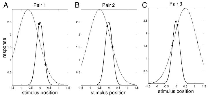
Knowing the difference in eye position provides important new constraints on the receptive field. •, the response of the neuron to a pair of stimuli, presented at 2 different positions on the screen. Three such pairs are shown. The curves show 2 possible Gaussians. · · ·, a possible receptive field which can explain pairs 2 and 3, provided there has been an eye movement between the 2 pairs. —, a possible RF which can explain both pairs on the assumption that the eyes have stayed at the fixation point throughout. Pairs 1 and 2 would have been sufficient to choose the — over the · · · without invoking any assumptions about eye movements. Over many pairs, this method will converge on a fit even if the assumed SD of eye position is implausibly large.

The preceding explanation ignored the possibility that eye movements might occur between the two members of a single pair. This is where the coil is critical. Having demonstrated that the coil probably reliably tells us differences in eye position between two trials, we can use the measured coil difference to correct for this. The mean eye position across the pair of trials is unknown, but in assessing the likelihood of the data given the currently postulated RF parameters, we integrate over all possible mean eye positions weighted by their a priori probability. The coil record suggests that mean eye position over a trial is normally distributed about the fixation point, so we modeled this probability as a Gaussian, with SD σe. The value of σ_e, plus the RF parameters, are free parameters in our fit: we select the values which lead to the highest likelihood of the observed data (maximum likelihood estimation, MLE). Simulations suggest that this approach can recover the correct parameters to within ~5% (the precise value depending on the number of trials, etc.).

Figure 8 shows the result of this new fitting procedure (“MLE-pairs”, —) for one cell, duf218. The results of the least-squares fit used so far in this paper (- - -) were shown, ignoring the problem of eye movements. The MLE-pairs method suggests a narrower RF of larger amplitude, exactly as one would expect if it has correctly taken into account the effects of eye movements. However, by itself this does not demonstrate that the method has correctly identified the underlying RF. Both methods give a good account of the mean firing rate as a function of position in the visual field, and many combinations of RF size and assumed eye-position variation could explain these data. Importantly, the combinations differ greatly in the variability in neuronal firing that they predict. According to the MLE-pairs fit, variation in eye position should add considerable variability to the spike counts in a way that depends on the stimulus location. Figure 8C compares the predicted and observed VMR. The close agreement is particularly striking because the MLE-pairs method does not explicitly fit these VMRs. Rather, the assumed combination of RF and eye movement that best explains the changes in firing rate between consecutive trials independently explains the observed VMR for each stimulus considered individually.

FIG. 8.

Reconstructing the RF of cell duf218. The different lines compare different approaches: LSQ: a least-squares fit to sqrt(spike count), ignoring eye movements and MLE-pair: a maximum-likelihood estimate using the coil to obtain the difference in eye position between consecutive pairs of stimuli, under the assumption that neuronal firing is Poisson, i.e., VMR = 1. A: underlying RF profile, as a function of position on the retina. B: square-mean-root (SMR) spike count (square of the expected value of the square-root of spike count) as a function of stimulus position on the screen. For the MLE-pair fit, this takes into account jitter in eye position, which is assumed to be Gaussian with the fitted SD. The experimentally observed SMR spike counts are shown with black disks (error bars, ±SE). C: variance:mean ratio.

Figure 9 examines how well the MLE-pairs fit explains the observed pattern of VMR across the population. For each cell, we calculated the correlation coefficient between the observed and predicted VMRs. This correlation was positive in 51/57 cells (P < 10⁻⁹, binomial distribution); the mean was 〈r〉 = 0.347 (significantly different from 0, P < 10⁻⁶, t-test). The cell shown in Fig. 8C is one of 15/57 in which this correlation was significant at the 5% level (it has r = 0.73). Given the noise associated with estimating variance, it is not surprising that the correlations are often small. The strong bias toward positive values is striking given that the model used in the fitting assumes that the variance of neuronal firing is proportional to the mean, so that, if it were not for eye movements, the expected correlation coefficient would be zero.

FIG. 9.

Distribution of the correlation coefficient between the variance: mean ratio (VMR) observed in the data and predicted by the MLE-pair fits over 57 cells. ▪, the 15 cells for which the correlation was significant at the 5% level. To reduce the noise, we restricted ourselves to stimulus positions with ≥10 repetitions (and, of course, mean >0). The number of points contributing to each correlation is thus rather small.

Figure 10 summarizes the MLE-pair estimates of RF size across the population, in the same way as Fig. 6 summarized the results of correcting for eye position using the coil. Once again, - - - shows the prediction from Eq. 3, where now σ_e and σ_RF are obtained from the MLE-pair fit. The agreement is much improved compared with Fig. 6. Whereas the “fractional changes” in Fig. 6 were scattered equally on either side of zero, now the change in SD is almost always negative, while that in amplitude is almost always positive (σ_RF < σ_obs for 51/57 cells, A_RF > A_obs for 51/57 cells, P < 10⁻⁶, binomial distribution; geometric mean σ_RF:σ_obs = 0.797, A_RF:A_obs = 1.35, both P < 10⁻⁶, t-test on log ratios). There is also a much clearer tendency for the changes to be larger where the jitter in eye position is large relative to the RF. Thus our MLE method incorporating eye jitter does result in systematically narrower SDs and larger amplitudes as expected if eye movements have been correctly accounted for and in contrast to the results of treating the coil as veridical. In addition, the agreement with the observed VMRs (Fig. 9) is powerful independent evidence that the fits are correctly estimating the extent of eye movements and the underlying RF size. However, before concluding that these estimates are correct, a number of properties are examined below to check their reliability.

FIG. 10.

Comparison of RF parameters obtained by MLE fits assuming no eye movements (σ_obs, A_obs) or assuming a Gaussian distribution of eye position (σ_RF, A_RF). Left: the ordinate is (σ²_RF ± σ²_obs)/(2σ_RF²), which is approximately the fractional change in RF SD between the 2 fits; right: (A_RF² − A_obs²)/(2A_RF²). In both plots, the abscissa is the ratio of the SD of eye jitter (σ_e, also obtained from the MLE-pair fit) to the SD of the fitted RF, σ_RF. In Fig. 6, all RF parameters were the result of a least-squares Gaussian fit to the sqrt(spike count), which is valid for any model of neuronal firing in which variance is proportional to mean. Here, σ_RF and A_RF were obtained from the MLE-pair fitting method under an assumption of Poissonian firing, in which the constant of proportionality is 1. To make a fair comparison with the prediction of Eq. 3 (- - -), we wanted the fits that produced (σ_obs, A_obs) and (σ_RF, A_RF) to differ only in their handling of eye movements not in their model of neuronal firing. In this plot, therefore σ_obs, A_obs were obtained with a maximum likelihood fit assuming Poissonian firing and no eye movements (Eq. 10). •, results for monkey Duf; ▪, monkey Ruf.

Checks and validation

FITTED SD OF EYE MOVEMENTS IS CONSISTENT WITH THE COIL

In the fitting procedure, we optimize to find the most likely SD of eye movements, σ_e. But if our assumptions are correct, and the coil accurately reports the difference in eye position between two consecutive trials, then we should be able to find σ_e by considering the distribution of those differences, Δc: we expect that σ_e ~ SD(Δc)/√2. Figure 11 compares this estimate of σ_e to the value obtained by the MLE fit, for each of our 57 cells. The two estimates are highly correlated (r = 0.89). This is further evidence supporting both our assumptions about the nature of the coil artifact and the success of the fitting procedure.

FIG. 11.

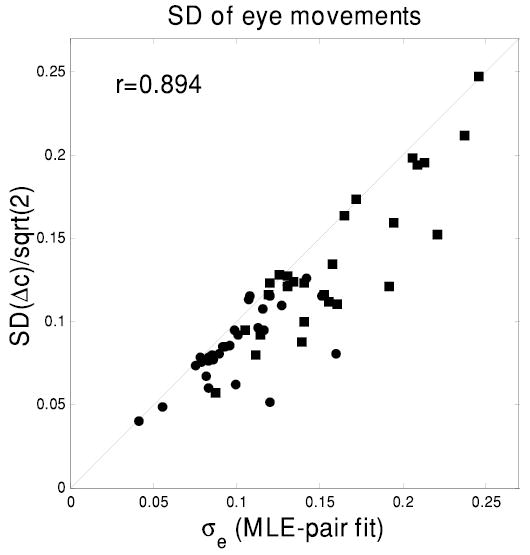
Comparing 2 different estimates for the SD of jitter in eye position, σ_e. The abscissa is the value produced by our MLE-pair fit. The ordinate is the SD of differences in the coil record between consecutive trials (assumed to reflect differences in eye position), divided by √2 to correct for the larger SD obtained by measuring differences. The correlation of 0.894 is highly significant (P < 10⁻⁶, n = 57 cells). The identity line is indicated. Both axes are in degrees. • results for monkey Duf; ▪, for monkey Ruf.

It is noticeable that the MLE estimate of σ_e tends to be slightly larger than expected from the coil differences. This is readily explained by assuming that the real value of eye position tend to be correlated from one 415-ms trial to the next. Under these circumstances, SD(Δc)/√2 will underestimate the true variation in eye position. Note that the suggestion that eye position is correlated from one trial to the next does not undermine our arguments that the drift artifact is also correlated from trial to trial. It is quite possible that both are correlated (although the correlation appears to be stronger for the artifact).

RESULTS ARE NOT SENSITIVE TO SMALL EYE MOVEMENTS DURING A TRIAL

The analysis presented in the APPENDIX implicitly assumes that the eye position remains constant throughout a trial. However, although the monkey was fixating, there may be microsaccades or significant drift in eye position during a trial. Our analysis is still valid, providing the mean spike count reflects the mean eye position during the trial. As a check that our results are not sensitive to eye movements that occur during a trial, we repeated our analysis, this time excluding all trials on which the SD of coil-measured eye position in the stimulated eye exceeded 0.05° over the course of the trial. The consequent reduction in the number of data points is exacerbated because, in our MLE-pair method, we restrict ourselves to considering consecutive pairs of trials. Thus for example, removing trials 30 and 32 due to excessive eye movement also results in the loss of trial 31. Five cells could not be analyzed because fewer than 10 pairs survived this culling. For the remaining 52 cells, the RF parameters were not significantly changed (for fitted RF SD, σ_RF, the correlation between the 2 sets of results is 0.953; geometric mean ratio is 0.967, no significant difference, t-test on log ratios (P = 0.09). For fitted RF amplitude, A_RF, these figures are 0.97, 1.01, P = 0.7). However, there was a small but significant reduction in the fitted SD of eye jitter, σ_e, by an average of 0.035° (correlation: 0.81).

RESULTS ARE NOT SENSITIVE TO THE EXACT MODEL OF SPIKE COUNTS

The results presented so far were based on a Poisson model of spike counts. This captures some aspects of our spike count statistics, such as the constant VMR, but is clearly oversimplistic. It is possible that the statistics we have assumed influenced our fit. The VMR of a Poisson process is exactly 1, whereas the VMRs observed in our spike counts are often higher by an order of magnitude. Our fits reproduce these large VMRs by postulating eye movements (Figs. 8 and 9). However, if our spike count model had larger intrinsic VMR, the MLE fit might produce smaller estimates of eye jitter. To find out whether our results were sensitive to the precise spike count model, we reran our fits using a bursty-Poisson model with VMR = 2 (see APPENDIX for details), a figure which is larger than most estimates for the VMR in cortical neurons (Britten et al. 1993; Dean 1981; Geisler and Albrecht 1997). This analysis used only trials where the SD of the coil measure over a single trial was <0.05°, as in the previous section. The results were extremely similar. The correlation between fitted RF SD for the 52 cells was 0.986; for fitted amplitude, 0.995; for σ_e, 0.969; the gradient of fitted regression lines did not differ significantly from 1 for any of these. There was some suggestion that the bursty Poisson model resulted in a marginally larger fitted RF SD, a smaller RF amplitude and a smaller σ_e, as expected from a model allowing more variance in the neuronal firing. However, these changes are extremely small (~1 spike/trial for RF amplitude, 0.01° for the SDs), demonstrating that our results are not unduly sensitive to the precise assumptions concerning neuronal firing. Similarly, simulations indicate that the results are not unduly sensitive to the exact shape of the RF. Even if the RF is not a Gaussian, if we define the best-fitting Gaussian to be that which would have been obtained by a least-squares fit if the eyes had been still, the MLE technique returns a good approximation to this best fit even when the simulated data have been contaminated by eye movements.

RESULTS ARE NOT SENSITIVE TO ADAPTATION

Neurons often show some response adaptation, which is a potential problem for our MLE-pair analysis. If the first stimulus in the pair elicited a particularly large response, the response to the second stimulus might be smaller than average, and this is not taken into account in our MLE fitting. However, it is not clear that response adaptation would cause any systematic errors as stimuli were presented in a random order. On any particular trial, the response is as likely to have been enhanced as suppressed by such a mechanism. The effect of adaptation is therefore primarily to increase the variance in neuronal firing, and we showed in the previous section that our results are not excessively sensitive to the precise assumptions about the variance of neuronal firing. Nevertheless, we verified explicitly that our fitting procedure is still valid given realistic amounts of adaptation.

One advantage of our short stimulus presentations (415 ms, with a gap of ≥100 ms between stimuli) is that strong adaptation is avoided. We examined the extent of adaptation in these data with a median-split analysis. We grouped pairs of trials according to the stimulus position for the second member of the pair and calculated the median value of the spikes elicited by the first member of the pair. We then calculated the mean of the square-root spike-count elicited by the second member, given that the first member of the pair had been greater/less than this median (m_> and m_≤, respectively). Across the population of cells, there was no tendency for the mean sqrt spike count to be smaller where the preceding trial had evoked a larger than median spike count, suggesting that little adaptation occurs (means could be evaluated for 562 stimulus positions in 57 neurons; m_> < m_≤ in 288/562 cases, P = 0.6, binomial; population average <m_> − m_≤ > = −0.072 ± 0.040 SE, not significantly different from 0, P = 0.07, t-test).

Even so, to evaluate the effect of any adaptation, we ran our MLE-fitting method on simulated data incorporating a simple model of adaptation. Whereas our MLE fit assumes that the spike count simply reflects the retinal position of the stimulus, our simulation reduced the elicited spikes by a “gain” factor depending on the number of spikes produced on the previous trial, N_prev: the gain was 1 if no spikes had been fired on the previous trial, and decreased linearly to zero with N_prev. We set this gain so as to obtain adaptation clearly stronger than that in most real cells (〈m_>− m_≤〉 = − 0.28). Our fitting procedure still extracted the correct parameters to within the same accuracy (~5%) as when no adaptation was included in the simulation.

SIMILAR FITS ARE PRODUCED WITHOUT USING COIL DATA AT ALL

We developed a second MLE method that makes no use of the coil at all (APPENDIX, Eq. A6). It simply looks at each individual spike count and considers how likely that spike count was given the postulated RF parameters and the postulated SD of eye jitter. Obviously, because this approach uses less information, it is not so well constrained. However, it has the advantage of being free of any assumptions concerning the coil.

The results are, again, extremely similar. The fitted amplitudes were marginally larger with the second MLE method (geometric mean ratio = 1.03, P = 0.02, t-test on log ratios), but the correlation between them was 0.99. There was no significant difference in either the SD of the RF or the SD of eye movements (correlations: 0.96 and 0.56, respectively, both highly significant, P < 10⁻⁵).

Estimates of eye position

An extension of our MLE-pair fitting also allows us to obtain an estimate of the eye position on individual trials (details in APPENDIX). After fitting the cell’s entire dataset to obtain the RF parameters and the SD of eye jitter, σ_e, we then run individual MLEs for each stimulus presentation in the cell’s dataset, in which we estimate the most likely eye position on that trial, given the RF parameters and eye jitter previously obtained.

These estimates of eye position are considerably more noisy than the estimates of RF parameters and eye jitter. There, five parameters are fitted, using hundreds of observations (on average 270 per cell). Here, a single parameter (the mean eye position across a pair of trials) is fitted to a pair of observations. When the observations do not tightly constrain the mean eye position, the a priori assumption that eye position is normally distributed about zero makes the MLE fit choose an eye position close to zero. Thus the MLE fit for eye position shows a slight bias toward zero, which emerges when we consider the population of fitted eye positions for a particular experiment. This is expected to be normally distributed with mean 0 and SD σ_e, where σ_e for this experiment has been obtained, along with the RF parameters, by the initial MLE-pair fit. In fact, over all 57 cells, the SD of the fitted eye positions is systematically about 0.014° less than σ_e, reflecting the bias toward zero.

Despite this, the fitted eye positions turn out to be well correlated with the values reported by the coil, even though these values were not used during the fit. Figure 12A shows this correlation for the cell examined in Fig. 8 (duf218). The shallow gradient, which was reflected across the population, again probably reflects the bias of the MLE fit toward small eye positions. The population mean of the correlation between the coil record and the fitted eye position over our 57 cells was 0.661, ranging from 0.28 to 0.90. This correlation was significant at the 5% level in all 57 cells, and at the 0.1% level in 54/57. This level of agreement, despite the bias in fitted eye positions and the artifact on the coil, is further evidence of the success of our MLE approach.

FIG. 12.

A: fitted eye position plotted against the eye position reported by the coil. B: the fitted eye position obtained from spikes recorded from a neighboring cell, duf218 2, plotted against the results from this cell. Here, we plot the mean eye position (average over 2 successive trials), because this 2-trial mean is the parameter which is estimated independently for each cell (see APPENDIX). In both panels, —, the regression line (fitted assuming ordinate and abscissa are subject to the same error); - - -, the identity; all axes are in degrees. The correlation coefficient and the number of samples are indicated on each panel. Both correlations were highly significant (P < 10⁻⁶).

Duf218 is a particularly interesting cell because spikes from a second cell, duf218 2, were recorded at the same time. Figure 12B compares the results of the fitted eye positions for the two cells. There is a significant correlation. This certainly shows that the estimate of eye position is not simply noise, although of course because estimates on both cells are subject to the same bias, it does not allow us to assess the absolute accuracy of the fit. We had six such pairs of simultaneously recorded cells. The mean correlation coefficient between the two estimates of eye position was 0.36, and the correlation was significant at the 1% level in 5/6 cell pairs.

Coil artifact

By a heuristic argument in the preceding text (Eq. 6), we arrived at estimates for the SD of the coil artifact and of eye movements σ_e, which were both ~0.11°. We can now compare these with the estimates from the MLE fits. The mean fitted σ_e is 0.128° (ranging from 0.041 to 0.246° with an SD of 0.045°). Figure 13 shows the SD of the coil record, SD(c), against the fitted SD of eye movements, σ_e. The coil record has larger SD for all but 6/57 cases. For 51 cells, therefore we can estimate the coil drift σ_n by assuming that var(c) = σ_e² + σ_n². The mean is 0.0952°, ranging from 0.0220 to 0.220° with an SD of 0.0467°.

FIG. 13.

Estimating the size of the search coil artifact. The abscissa is the estimate of the SD of eye jitter, σ_e, produced by our MLE-pair fit. The ordinate is the SD of the coil record for each cell, which is presumed to reflect not only the extent of eye jitter, σ_e but also the artifact on the coil. The correlation of 0.808 is highly significant (P < 10⁻⁶, n = 57 cells). The identity line is indicated. Both axes are in degrees. •, results for monkey Duf; ▪, for monkey Ruf.

As an alternative estimate, if we assume that our MLE technique has successfully recovered the eye positions on each trial, then subtracting the fitted eye position from the coil record gives us a trial-by-trial estimate of the drift on the coil, which works for all 57 cells. The population average SD of the deduced coil drift is 0.116° (ranging from 0.052 to 0.217° with an SD of 0.042°). All three different estimates are in good agreement. They suggest that the drift on scleral search coils is of approximately the same magnitude as fixational eye movements, with an SD of ~0.1°.

DISCUSSION

It is widely believed that visual receptive fields in primary visual cortex are fixed in retinal coordinates and hence change their spatial location when the eyes move. Although one early report suggested that there might be dynamic compensation for fixational eye movements (Motter and Poggio 1990), a series of studies by Gur and Snodderly (Gur and Snodderly 1997; Gur et al. 1997) provided compelling evidence to the contrary. Our demonstration of a relationship between spike count variability and stimulus location further reinforces the view that RFs are fixed in retinal coordinates. When the stimulus was presented at a location where the RF was most sensitive to small displacements, spike count variability was systematically larger than at less sensitive locations. Importantly, this demonstrates the effect of retinally fixed RFs without relying on measures of eye position at all.

Because RFs are fixed on the retina, changes in eye position will interfere with the estimation of RF size and shape. Some studies have attempted to estimate the retinal location of each stimulus simply by combining knowledge of the spatial location with measures of eye position (Conway 2001; Livingstone 1998; Livingstone and Tsao 1999; Livingstone et al. 1996). This places high reliance on the accuracy of these records over extended periods, yet no one to our knowledge has demonstrated such accuracy with any system. Furthermore, none of the studies that have applied eye-position correction to stimulus locations have evaluated the effectiveness of the procedure (e.g., by comparing data with and without correction). We find that applying eye-position correction did not in general produce smaller RF estimates. Taken together, these observations suggest that a substantial fraction of the measured variation in eye position is artifactual. This raises serious problems of interpretation for those studies that have applied eye-position correction without evidence of its effectiveness.

It is unclear what the source of these artifacts is. It does not appear to be a property of the electronics—we found that signals from calibration coils were stable to within very narrow limits over many hours. This was true even when a calibration coil was placed next to a working animal, so it is unlikely that the artifact is due to alterations in the field induced by postural changes. One important factor may be that coils implanted in animals are not rigidly mounted. Mechanical distortion of the coil or of the connecting wire, due to movements of the eyelids, brow, or temporal muscles, could give rise to changes in recorded position in the absence of an eye movement. Indeed, the fact that blinks are associated with substantial transients in the signal from search coils seems clear evidence that changes in lid tension can introduce artifacts in the position signal. To what extent these artifacts are reduced if the coils are sutured to the globe will require further investigation.

The fact that scleral search coil measures contain substantial artifactual variation is particularly problematic for binocular measures. A number of human studies have reported that the vergence angle between the eyes is much less variable than conjugate eye position during fixation. If the same holds for monkeys, it would mean that the real variation in vergence would be substantially smaller than this artifact and hence very hard to estimate. Several of our observations indicate that this is indeed the case. 1) When monocular RF sizes were estimated with eye-position correction, the results were very similar whether the eye-position measure used was that of the stimulated eye or the nonstimulated eye. 2) The analysis of spike count variability in disparity selective neurons showed that the variability increases only in regions of extremely steep disparity tuning, suggesting a vergence SD of 1 min arc. This is in good agreement with values from human studies. 3) The measured SD of vergence is similar in magnitude to our estimates of the artifactual coil drift. And 4) the differences between two coils implanted in one eye were similar to those for vergence, both in absolute magnitude and in their temporal structure (they had nearly identical Fourier amplitude spectra). We conclude that binocular coils overestimate vergence variability. In fact, very few studies of binocular neurons have included quantitative analysis of vergence variability (Cumming 2002; Prince et al. 2002a). The results presented here suggest that vergence variability poses even less of a problem than such measures indicated.

Note that the coil artifact does not render the measurement of vergence altogether invalid. Reliable measures of vergence velocity are still possible (Busettini et al. 1996, 2001). Furthermore, if two conditions are interleaved, vergence measures can still reliably detect any systematic change between them (Cumming and Parker 1999; Thomas et al. 2002). Any systematic changes in vergence with the stimulus condition [e.g., changes in fixation distance (Trotter et al. 1992, 1996)] might influence the response of binocular neurons. Without vergence measures, these changes might be interpreted as a property of the neuron itself.

That there is both real and artifactual variation in the eye-position records from fixating monkeys poses a significant problem for estimating RF size at least for studies of foveal V1. This in turn makes it difficult to be confident that any stimulus is confined to within a single RF or that a stimulus that elicits some contextual modulation really remains outside the receptive field. However, our data suggest that the artifactual component is correlated across successive trials, and the influence on RF measures can be substantially reduced by considering the differences in reported eye position between consecutive trials. We therefore developed a new method of analysis, which examines pairs of stimuli and uses the two firing rates, in conjunction with the change in stimulus location, to estimate RF size in a way which is not disrupted by changes in eye position over time. A number of checks suggest that this approach can successfully estimate the RF parameters and amount of eye jitter, that it is not disrupted by small eye movements which occur during a trial or by errors remaining in the coil difference signal, and that it is not unduly sensitive to the precise model assumptions. This technique yielded systematically smaller RF estimates than methods that either ignore eye movements or assume the coil is veridical, it explained the observed variability of neuronal discharge, and it was able to match estimates of eye-position variability derived from the coil in a way that was not sensitive to slow drifts. Thus in every way we have examined, it behaves as if it has correctly separated the underlying RF and the influence of eye movements on the neuronal response.

This is important not only because it allows estimation of RF size in V1 of the awake monkey, but also because it provides a method by which the absolute accuracy of an eye-position recording technique can be assessed. If, for example, suturing the coil to the globe reduces these artifactual drifts, this can now be demonstrated using our MLE-pair technique. Additionally, we have argued in the preceding text that actual variations in vergence are very small so that measurements of vergence effectively give a direct estimate of the artifact. Thus if some eye-position recording technique produced vergence SDs of a few minutes of arc and the MLE-pair method indicated a small artifact, this would show beyond reasonable doubt that the measure of eye position was accurate.

APPENDIX: MAXIMUM LIKELIHOOD ESTIMATION OF RECEPTIVE FIELD PARAMETERS AND EYE MOVEMENTS

The mean spike count, n, observed during a trial depends on the position r of the stimulus with respect to the receptive field (RF). This in turn depends on the stimulus’ position on the screen, s, and the position of the eye relative to the fixation point, e (Fig. A1)

FIG. A1.

The relationship between the position of the stimulus on the screen, s, and its image on the retina, r.

$$r=s-e$$ (A1)

In talking of the position of the eye during a trial, we are ignoring the possibility that eye movements occur within a trial. More realistically, e represents the average eye position over a trial, and we are assuming that the expected spike count, n, reflects the average retinal position r. (In the text, we present evidence that this assumption is sufficiently accurate.)

The RF is assumed to be Gaussian, i.e.

$$n(r)=B+A\mathrm{\hspace{0.17em} }exp(-{(r-c)}^2/2{\sigma }^2)$$ (A2)

where A is the RF amplitude, expressed as the mean number of spikes evoked by an optimally-placed stimulus, σ is the RF SD, c is the center of the receptive field in retinal coordinates, and B is the baseline spike count. Note that the only assumption we make about the response of these neurons is that it is a Gaussian function of position. Our analysis holds irrespective of any nonlinearities which may contribute to this response.

Usually, the spike counts were assumed to be Poisson, so that the probability of recording N spikes during a trial is

$$P_{\text{spike}}(N,n)=\frac{n^N}{N!}\mathrm{\hspace{0.17em} }exp(-n)$$ (A3)

We also investigated the effects of modeling the spike counts as a bursty Poisson. Here, bursts are generated as a Poisson process, and each burst consists of m spikes, where m in turn has a Poisson distribution. The spike count model thus has two free parameters: the mean number of bursts per trial, $\overline{n}$, and the mean number of spikes per burst, $\overline{m}$. The mean spike count per trial is $\overline{mn}$, and the variance:mean ratio is $1+\overline{m}$. We set $\overline{m}=1$ to obtain a VMR of 2. In this case, the probability of recording N spikes during a trial was obtained by numerical inversion of the generating function.

If retinal position was known

If either the scleral search coil or the animal’s fixation were known to be flawless, we would know the retinal position r for each stimulus. Then for a particular set of RF parameters we can deduce the expected spike count n(r) (Eq. A2), and hence the probability of observing a particular number of spikes N. The likelihood L of the entire data set is therefore, assuming results from different trials j are independent

$$L(A,\mathrm{\hspace{0.17em} }B,\mathrm{\hspace{0.17em} }c,\mathrm{\hspace{0.17em} }\sigma )=\prod _j{P}_{\text{spike}}(N_j,\mathrm{\hspace{0.17em} }n(r_j))$$ (A4)

where the argument indicates that the likelihood depends on the RF parameters A, B, c, σ. We would estimate these parameters by adjusting them so as to maximize this likelihood.

Using information from the coil (MLE-pair)

In practice, fixation is not perfect and scleral search coils appear to be subject to an artifact. However, we can still obtain a well-constrained fit if we assume that the scleral search coil accurately reports changes in eye position over a sub-second timescale, although the actual values may be subject to a slow drift which means they cannot be relied on over the course of an experiment. (Evidence supporting this assumption is discussed in the text.)

Rather than using data-points individually, we therefore use them in pairs. We assess the probability of recording N₁ counts for a stimulus at screen position s₁, followed by N₂ counts for a stimulus at s₂. From the coil, we know the change in eye position, Δe = e₂ − e₁, so we simply need to integrate over all possibilities for the mean eye position averaged over both trials, ē = (e₁+e₂)/2. This is distributed normally with SD σ_e/√2, so

$$\begin{array}{l}P\{N_1,\mathrm{\hspace{0.17em} }{N}_2|s_1,\mathrm{\hspace{0.17em} }{s}_2,\mathrm{\hspace{0.17em} }\mathrm{\Delta }e\}=\frac{1}{{\sigma }_e\sqrt{\pi }}\int \text{d}\overline{e}exp(-{\overline{e}}^2/{\sigma }_{\text{e}}^2)\\ \times \mathrm{\hspace{0.17em} }{P}_{\text{spike}}(N_1,\mathrm{\hspace{0.17em} }n(s_1-\overline{e}+\mathrm{\Delta }e/2))P_{\text{spike}}(N_2,\mathrm{\hspace{0.17em} }n(s_2-\overline{e}-\mathrm{\Delta }e/2))\end{array}$$

Re-expressing our data as a set of consecutive pairs of trials, the likelihood of the dataset is

$$\text{L}(A,\mathrm{\hspace{0.17em} }B,\mathrm{\hspace{0.17em} }c,\mathrm{\hspace{0.17em} }\sigma ,\mathrm{\hspace{0.17em} }{\sigma }_e)=\prod _{j}P\{N_{1j},\mathrm{\hspace{0.17em} }{N}_{2j}|s_{1j},\mathrm{\hspace{0.17em} }{s}_{2j},\mathrm{\hspace{0.17em} }\mathrm{\Delta }{e}_j\}$$ (A5)

We fit the whole data-set for the RF parameters and for σ_e.

It is also of interest to obtain an estimate of the eye position on each trial. In practice, we do this by obtaining an estimate of the average eye position ē in each pair of trials (because the difference Δe is known, this tells us the eye position for each trial). For the jth pair of trials, we seek ē_j that maximizes

$$\begin{array}{l}P\{N_{1j},\mathrm{\hspace{0.17em} }{N}_{2j}|s_{1j},\mathrm{\hspace{0.17em} }{s}_{2j},\mathrm{\hspace{0.17em} }\mathrm{\Delta }{e}_j\}=\frac{1}{{\sigma }_e\sqrt{\pi }}exp(-{\overline{e}}_j^2/{\sigma }_e^2)\\ \times \mathrm{\hspace{0.17em} }{P}_{\text{spike}}(N_{1j},\mathrm{\hspace{0.17em} }n(s_{1j}-{\overline{e}}_j+\mathrm{\Delta }{e}_j/2))P_{\text{spike}}(N_{2j},\mathrm{\hspace{0.17em} }n(s_2-{\overline{e}}_j-\mathrm{\Delta }{e}_j/2))\end{array}$$

We then obtain the eye position on the first and second members of the pair

$$e_{1j}={\overline{e}}_j-\mathrm{\Delta }{e}_j/2,\mathrm{\hspace{0.17em} }{e}_{2j}={\overline{e}}_j+\mathrm{\Delta }{e}_j/2$$

In expressing our data as a set of consecutive pairs of trials, the same trial often occurs as a member of two pairs. Strictly, this invalidates Eq. A5, because this assumes that all the pairs are independent. We ignored this complication. For the duplicated trials, we took the final fitted eye position to be the mean of the two estimates e_1j and e_2,j−1.

To derive the expected spike count for comparison with experimental observations, we have to incorporate the differences Δe that were used in fitting. The easiest way to do this is by simulation. For each pair, we pick ē randomly from a normal distribution with SD σ_e/√2. Given Δe from the coil, this specifies e₁ and e₂ and hence the position of the stimuli on the retina. The RF function specifies the expected number of spikes on each trial, and the actual number was drawn from a Poisson distribution with this mean. Repeating this many thousands of times for every pair used in fitting allows us to determine the expected spike count distribution, and the VMR, for each stimulus screen position used.

Without using the coil

We also developed a method of estimating RF parameters in the presence of eye movements that makes no use of data from the search coil. Here, we simply seek to maximize the likelihood of obtaining the observed spike counts as a function of position without including any constraints from the coil. To estimate the probability of observing a particular spike count, N, given a stimulus screen position s, we must integrate over all possible eye positions e, weighted by their probability of occurring. As before, we assume that the distribution of eye positions, along the axis that stimulus position is varying, is Gaussian with SD σ_e, where σ_e is an additional parameter to be fit. Then

$$Pr\left\{N_j\right|s_j\}=\prod _j\frac{1}{{\sigma }_e\sqrt{2\pi }}{\int }_{-\infty }^{+\infty }\text{d}{e}_{j}exp(-e_j^2/2{\sigma }_e^2)P_{\text{spike}}(N_j,n(s_j-e_j))$$ (A6)

and the likelihood L(A,B,c,σ,σ_e) is given by the product over all trials j.

References

- Britten KH, Shadlen MN, Newsome WT, Movshon JA. Responses of neurons in macaque MT to stochastic motion signals. Vis Neurosci. 1993;10:1157–1169. doi: 10.1017/s0952523800010269. [DOI] [PubMed] [Google Scholar]
- Busettini C, Fitzgibbon EJ, Miles FA. Short-latency disparity vergence in humans. J Neurophysiol. 2001;85:1129–1152. doi: 10.1152/jn.2001.85.3.1129. [DOI] [PubMed] [Google Scholar]
- Busettini C, Miles FA, Krauzlis RJ. Short-latency disparity vergence responses and their dependence on a prior saccadic eye movement. J Neurophysiol. 1996;75:1392–1410. doi: 10.1152/jn.1996.75.4.1392. [DOI] [PubMed] [Google Scholar]
- Collewijn H, Erkelens CJ, Steinman RM. Binocular co-ordination of human horizontal saccadic eye movements. J Physiol. 1988;404:157–182. doi: 10.1113/jphysiol.1988.sp017284. [DOI] [PMC free article] [PubMed] [Google Scholar]
- Conway BR. Spatial structure of cone inputs to color cells in alert macaque primary visual cortex (V-1) J Neurosci. 2001;21:2768–2783. doi: 10.1523/JNEUROSCI.21-08-02768.2001. [DOI] [PMC free article] [PubMed] [Google Scholar]
- Cumming BG. An unexpected specialization for horizontal disparity in primate primary visual cortex. Nature. 2002;418:633– 636. doi: 10.1038/nature00909. [DOI] [PubMed] [Google Scholar]
- Cumming BG, Parker AJ. Binocular neurons in V1 of awake monkeys are selective for absolute, not relative, disparity. J Neurosci. 1999;19:5602–5618. doi: 10.1523/JNEUROSCI.19-13-05602.1999. [DOI] [PMC free article] [PubMed] [Google Scholar]
- Dean AF. The variability of discharge of simple cells in the cat striate cortex. Exp Brain Res. 1981;44:437– 440. doi: 10.1007/BF00238837. [DOI] [PubMed] [Google Scholar]
- Duwaer AL. New measures of fixation disparty in the diagnosis of binocular oculomotor deficiences. Am J Optom Physiol Opt. 1983;60:586–597. doi: 10.1097/00006324-198307000-00006. [DOI] [PubMed] [Google Scholar]
- Enright JT. Exploring the third dimension with eye movements: better than stereopsis. Vision Res. 1991;31:1549–1562. doi: 10.1016/0042-6989(91)90132-o. [DOI] [PubMed] [Google Scholar]
- Geisler WS, Albrecht DG. Visual cortex neurons in monkeys and cats: detection, discrimination, and identification. Vis Neurosci. 1997;14:897–919. doi: 10.1017/s0952523800011627. [DOI] [PubMed] [Google Scholar]
- Gur M, Beylin A, Snodderly DM. Response variability of neurons in primary visual cortex (V1) of alert monkeys. J Neurosci. 1997;17:2914–2920. doi: 10.1523/JNEUROSCI.17-08-02914.1997. [DOI] [PMC free article] [PubMed] [Google Scholar]
- Gur M, Snodderly DM. Studying striate cortex neurons in behaving monkeys: benefits of image stabilization. Vision Res. 1987;27:2081–2087. doi: 10.1016/0042-6989(87)90122-2. [DOI] [PubMed] [Google Scholar]
- Gur M, Snodderly DM. Visual receptive fields of neurons in primary visual cortex (V1) move in space with the eye movements of fixation. Vision Res. 1997;37:257–265. doi: 10.1016/s0042-6989(96)00182-4. [DOI] [PubMed] [Google Scholar]
- Jaschinski-Kruza W, Schubert-Alshuth E. Variability of fixation disparity and accommodation when viewing a CRT visual display unit. Ophthalmic Physiol Opt. 1992;12:411– 419. [PubMed] [Google Scholar]
- Judge SJ, Richmond BJ, Chu FC. Implantation of magnetic search coils for measurement of eye position: an improved method. Vision Res. 1980;20:535–538. doi: 10.1016/0042-6989(80)90128-5. [DOI] [PubMed] [Google Scholar]
- Kagan I, Gur M, Snodderly DM. Spatial organization of receptive fields of V1 neurons of alert monkeys: comparison with responses to gratings. J Neurophysiol. 2002;88:2557–2574. doi: 10.1152/jn.00858.2001. [DOI] [PubMed] [Google Scholar]
- Livingstone MS. Mechanisms of direction selectivity in macaque V1. Neuron. 1998;20:509–526. doi: 10.1016/s0896-6273(00)80991-5. [DOI] [PubMed] [Google Scholar]
- Livingstone M, Freeman D, Hubel D. Visual responses in V1 of freely viewing monkeys. Cold Spring Harb Symp Quant Biol. 1996;61:27–37. [PubMed] [Google Scholar]
- Livingstone MS, Tsao DY. Receptive fields of disparity-selective neurons in macaque striate cortex. Nat Neurosci. 1999;2:825– 832. doi: 10.1038/12199. [DOI] [PubMed] [Google Scholar]
- Motter BC, Poggio GF. Dynamic stabilization of receptive fields of cortical neurons (VI) during fixation of gaze in the macaque. Exp Brain Res. 1990;83:37– 43. doi: 10.1007/BF00232191. [DOI] [PubMed] [Google Scholar]
- Ogle K.Researches in Binocular Vision. New York: Hafner, 1964.
- Prince SJ, Cumming BG, Parker AJ. Range and mechanism of encoding of horizontal disparity in macaque V1. J Neurophysiol. 2002a;87:209–221. doi: 10.1152/jn.00466.2000. [DOI] [PubMed] [Google Scholar]
- Prince SJ, Pointon AD, Cumming BG, Parker AJ. Quantitative analysis of the responses of V1 neurons to horizontal disparity in dynamic random-dot stereograms. J Neurophysiol. 2002b;87:191–208. doi: 10.1152/jn.00465.2000. [DOI] [PubMed] [Google Scholar]
- Riggs L, Neill E. Eye movements recorded during convergence and divergence. J Opt Soc Am A. 1960;50:913–920. [Google Scholar]
- Snodderly DM, Gur M. Organization of striate cortex of alert, trained monkeys (Macaca fascicularis): ongoing activity, stimulus selectivity, and widths of receptive field activating regions. J Neurophysiol. 1995;74:2100–2125. doi: 10.1152/jn.1995.74.5.2100. [DOI] [PubMed] [Google Scholar]
- St Cyr GJ, Fender DH. The interplay of drifts and flicks in binocular fixation. Vision Res. 1969;9:245–265. doi: 10.1016/0042-6989(69)90004-2. [DOI] [PubMed] [Google Scholar]
- Thomas OM, Cumming BG, Parker AJ. A specialization for relative disparity in V2. Nat Neurosci. 2002;5:472– 478. doi: 10.1038/nn837. [DOI] [PubMed] [Google Scholar]
- Trotter Y, Celebrini S, Stricanne B, Thorpe S, Imbert M. Modulation of neural stereoscopic processing in primate area V1 by the viewing distance. Science. 1992;257:1279–1281. doi: 10.1126/science.1519066. [DOI] [PubMed] [Google Scholar]
- Trotter Y, Celebrini S, Stricanne B, Thorpe S, Imbert M. Neural processing of stereopsis as a function of viewing distance in primate visual cortical area V1. J Neurophysiol. 1996;76:2872–2885. doi: 10.1152/jn.1996.76.5.2872. [DOI] [PubMed] [Google Scholar]
- Tsao DY, Livingstone MS. Receptive fields of disparity-tuned simple cell in macaque V1. Neuron. 2003;38:103–114. doi: 10.1016/s0896-6273(03)00150-8. [DOI] [PMC free article] [PubMed] [Google Scholar]