

Abstract
Optimal performance in two-alternative, free response decision making tasks can be achieved by the drift-diffusion model of decision making - which can be implemented in a neural network - as long as the threshold parameter of that model can be adapted to different task conditions. Evidence exists that people seek to maximize reward in such tasks by modulating response thresholds. However, few models have been proposed for threshold adaptation, and none have been implemented using neurally plausible mechanisms. Here we propose a neural network that adapts thresholds in order to maximize reward rate. The model makes predictions regarding optimal performance and provides a benchmark against which actual performance can be compared, as well as testable predictions about the way in which reward rate may be encoded by neural mechanisms.
Keywords: reinforcement learning, drift-diffusion, decision making, stochastic optimization
1 Introduction and background
A tradeoff between speed and accuracy is one of the hallmarks of human performance in cognitive tasks. Typically observed in controlled behavioral experiments in which participants are encouraged to respond quickly, the concept formalizes the common sense notion that rushing produces more mistakes. Despite the pervasive nature of this phenomenon and the longstanding recognition of it, relatively little research has addressed how organisms address the balance between speed and accuracy. Nevertheless, any successful model of the physical mechanisms underlying decision making will ultimately need to account for the speed-accuracy tradeoff: why does a tradeoff occur at all, and how do organisms change that tradeoff as conditions change?
In abstract models of decision making, especially those addressing two-alternative forced choice (TAFC) tasks, the speed-accuracy tradeoff has traditionally been explained in terms of a task-dependent decision criterion, or threshold for termination of the decision-making process. This process is typically described as a progressive accumulation of evidence for each of the alternatives, the decision being made when the evidence in favor of one alternative versus the other exceeds the threshold (Laming, 1968; Luce, 1986; Ratcliff, 1978). If the threshold is low, the decision will be made quickly, but will be subject to noise. If the threshold is high, the decision process will take longer but will have greater time to ‘average out’ the effects of noise and therefore be more accurate. While a number of neural network models have addressed the mechanisms underlying TAFC task performance (e.g., Botvinick, Braver, Barch, Carter & Cohen, 2001; Brody, Hernandez, Zainos & Romo, 2003; Grossberg & Gutowski, 1987; Usher & McClelland, 2001; Wang, 2002), thresholds in these models have typically been modeled simply as assigned parameters rather than as neural mechanisms in their own right.
Here we propose an explicit set of neural mechanisms by which thresholds may be implemented and adapted to maximize reward rate. We do this by building on existing models of TAFC decision making that involve competing accumulators of evidence, one for each possible action. To each accumulator we add a mechanism for implementing a response threshold: a unit with a high-gain, sigmoidal activation function that approximates a step function. We propose that such units control response initiation, and that they are triggered by critical levels of accumulated evidence in the accumulator units. We then define an algorithm for modulating thresholds and describe its implementation using a neurally plausible mechanism. The model consists of a set of stochastic differential equations that is equivalent to a classic connectionist recurrent neural network with five units. In sections 2 and 3 we review relevant background before describing the model in sections 4 – 6. We conclude with a discussion in Section 7.
2 The drift diffusion model (DDM)
Sequential sampling models of decision making have long provided accounts of many regularities in response time (RT) and accuracy data in choice-reaction experiments (Luce, 1986). In sequential sampling, the stimulus is assumed to be a sequence of samples from one of two possible distributions, as, for example, in Fig. 7.2A. To determine which distribution is actually generating the stimulus, sampling is repeated and evidence in favor of one or another hypothesis is accumulated until a response criterion has been reached. Speed-accuracy tradeoffs can be explained in such models by shifts in the response threshold toward or away from the starting points of the decision variables: closer thresholds mean shorter RTs and higher error rates on average (Laming, 1968; Ratcliff, 1978).
Figure 7.
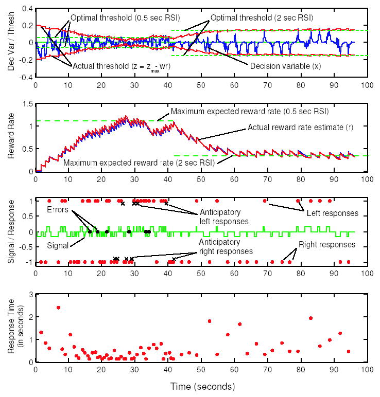
Timecourses of variables in a sample run of the algorithm. The DDM (Eq. 1) is simulated directly in the top timecourse, where the decision variable traces out a trajectory within bounds formed by the dynamic threshold (each point of contact between these represents a decision). Optimum thresholds for the two RSI conditions simulated (0.5 sec RSI, until about t ≈ 42 secs; 2 sec RSI, from 42 secs to end) are shown as dashed lines. Second timecourse shows leaky integrator estimate of reward rate (Eq. 11), superimposed on an estimate with added Gaussian noise, plus dashed lines indicating the expected reward rate for the optimum threshold in each RSI condition. Third plot shows signal direction (upward square pulse = left; zero = RSI; downward square pulse = right; responses are dots plotted at height 1 for left and −1 for right; dots at height 0 are premature responses occurring due to low threshold, and x’s denote errors. Fourth plot shows RTs.
In random walk versions of TAFC sequential sampling models, each evidential increment for one hypothesis reduces the evidence in favor of the other so that there is only a single decision variable: the difference in accumulated evidence for each hypothesis. (Fig. 7.2B shows this variable plotted against time for four different decisions. Fig. 7.2C shows the resulting response time distributions over many decisions.) Steps in the random walk are equivalent to increments of the total log-likelihood ratio for one hypothesis over the other, making the model equivalent to the sequential probability ratio test (SPRT) (Laming, 1968). This is theoretically appealing as a starting point for investigating the role of reward in decision making, because the SPRT is optimal in the sense that no other test can achieve higher expected accuracy in the same expected time, or, conversely, reach a decision faster for a given level of accuracy (Wald & Wolfowitz, 1948). However, the SPRT does not specify the optimal threshold for maximizing other values of potential interest, such as reward rate.
The drift-diffusion model (DDM) (Ratcliff, 1978; Smith & Ratcliff, 2004; Stone, 1960) is a version of the SPRT in which stimuli are sampled continuously rather than at discrete intervals. The difference between the means of the two possible stimulus distributions (see Fig. 7.2A), imposes a constant drift of net evidence toward one threshold, and the variance imposes a Brownian motion that may lead to errors. In monkeys, the continuously evolving firing rates of neurons in the lateral intraparietal sulcus (area LIP) have been related to competing accumulators that approximate the drift-diffusion process in oculomotor tasks (Gold & Shadlen, 2001; Roitman & Shadlen, 2002, Shadlen & Newsome, 2001). Similar findings have been reported for frontal structures responsible for controlling eye movements (Hanes & Schall, 1996). Importantly, as shown in section 3, the expected reward rate can be computed for the DDM (Gold & Shadlen, 2002), allowing learning mechanisms to be analyzed in terms of a well-defined optimization problem (Bogacz, Brown, Moehlis, Holmes & Cohen, in review).
The DDM is defined as the stochastic differential equation (SDE)
| (1) |
where A is the signal strength, dW denotes increments of an independently and identically distributed (i.i.d.) Wiener (white noise) process and factor c weights the effect of noise. At any given moment, the distribution of possible positions of a particle moving in one dimension and governed purely by a Wiener process is given by a Gaussian distribution whose mean is the starting point of the particle (in our case, the decision variable), and whose variance is equal to the time elapsed since the start of the process. Brownian motion of this type causes diffusion of a substance within a liquid, from whence comes the term ‘diffusion’ in the name of the model. Nonzero drift A contributes a tendency for trajectories to move in the direction of the drift, producing a corresponding linear movement in the mean of the particle position distribution over time. Below, we will use the terms ‘drift’ and ‘signal’ interchangeably.
For models of this type to explain effects that are observed in human performance - including the speed-accuracy tradeoff, sequential effects such as post-error slowing, and speeded response to frequent stimulus alternations and repetitions (Luce, 1986) - their parameters must be adaptive on a short time-scale. Traditionally, parameters have been inferred by fits to behavioral data, and additional degrees of freedom have been added to models to explain different behavioral phenomena (e.g., Ratcliff & Rouder, 1998). However, in order to go beyond identifying the relevant degrees of freedom and toward the principles that govern the selection of specific parameter values, several questions left unanswered by this approach must be addressed. For example, on what basis do subjects select particular parameter values of the decision process (e.g., starting point or initial value of the decision variable, and threshold for termination)? Are subjects behaving so as to minimize errors, to maximize reward rate, or to do something else altogether? How are their parameters modified in response to ongoing experience? Only a limited number of studies have addressed these questions and, to our knowledge, none have addressed the question of neural implementation.
Below, we propose a neural network model that explains how the decision threshold can be adapted (and a tradeoff between speed and accuracy chosen) in order to maximize reward rate over multiple trials. This is based on a simple neural network model that implements the DDM, as described in the next section.
2.1 Neural implementation of the DDM
The accumulation of evidence in the DDM can be approximated by a simple neural network with two ‘decision’ units, each of which is assumed to be preferentially sensitive to one of the stimuli and also to be subject to inhibition from the other unit (see Fig. 7.2D), as proposed by Usher & McClelland (2001) (cf. Bogacz et al., in review; Gold & Shadlen, 2002). Each unit has a leak term, and therefore accumulates evidence for its corresponding stimulus subject to decay over time, while competing with the unit representing the other decision alternative. We and others have shown that, with suitable parameter choices, this model closely approximates the DDM.
Specifically, the evolving activation of each unit (indexed by i) is determined by an SDE, the deterministic part of which is:
| (2) |
where Ii is the input, usually assumed to be a step function of time (corresponding to stimulus onset) and −βyj represents inhibition from the other unit(s). With the stochastic component of the activation function included, the pair of units is governed by;
| (3) |
| (4) |
Here we assume linear or piecewise linear activation functions for ease of analysis (we will abandon this when we discuss threshold-crossing detectors, a case in which nonlinearity is critical). This assumption provides a useful approximation to a more realistic, sigmoid function (Cohen & Grossberg, 1983; Freeman, 1979) and is also consistent with the idea that attention acts to place processing units in their central, approximately linear range, where they are most sensitive to afferent input (Cohen, Dunbar & McClelland, 1990). Sigmoids saturate near 0 at a small, positive baseline value, and also near a finite maximum which is typically rescaled to 1, thus avoiding the implausibilities of potentially unbounded or negative activations. For such units each equation of (3–4) takes the form:
| (5) |
Summing the noise-free linearized equations (3) and (4), we find that solutions approach an attracting line y1 + y2 = (I1 + I2)/(1 + β) exponentially fast at rate 1 + β. Differencing them yields an Ornstein-Uhlenbeck process for the net accumulated evidence x = y1 − y2:
| (6) |
If leakage and inhibition are balanced (β = 1) this becomes the DDM (Eq. 1) with A = I1 − I2 representing the difference in inputs. See Bogacz et al. (in review), Brown, Gao, Holmes, Bogacz, Gilzenrat and Cohen (2005) and Holmes, Brown, Moehlis, Bogacz, Gao, Aston-Jones, Rajkowski and Cohen (2005) for further details and verification that the nonlinear system approximates this behavior.
Fig. 7.2F shows the evolution of the activations y1(t) and y2(t) over time. After stimulus onset, the system state (y1, y2) approaches the attracting line along which slower, diffusive behavior occurs as the state approaches one or another boundary under the influence of the noisy signal. Projection of the state (y1, y2) onto this line yields the net accumulated evidence x(t), which approximates the DDM as shown in Fig. 7.2B.
3 A free-response, two alternative forced choice task
To investigate the hypothesis that speed-accuracy tradeoffs are driven by a process of reward maximization, we consider an experiment in which subjects try to determine the direction of motion of moving dots on a screen, as in Roitman & Shadlen (2002). They are free to respond at any time after stimulus presentation, and a response terminates the stimulus. Initial results from such an experiment suggest that people adapt their speed-accuracy tradeoffs in a manner consistent with the goal of maximizing reward, and that this adaptation can happen quite quickly (Bogacz et al., in review; Simen, Holmes & Cohen, 2005). People can also adapt their speed-accuracy tradeoffs in similar tasks in response to explicit instructions (Palmer, Huk & Shadlen, 2005).
To provide a benchmark against which to measure evidence of adaptive behavior, we first describe optimal performance under this experimental paradigm. Assuming a constant rate of trial presentation, the expected reward rate over a sequence of trials in which correct responses are rewarded by 1 unit and errors by 0 can be expressed as follows (Gold & Shadlen, 2002):
| (7) |
Here ER is the expected error rate (proportion of errors), DT is the decision time, T0 is the residual latency (non-decision-making component of response time comprising stimulus encoding and motor execution times), and RSI is the response-stimulus interval (wait time from the last response to the next stimulus onset).
For the DDM, ER and DT, and hence RR, depend only on the signal-to-noise ratio A/c and threshold-to-signal ratio z/A, and we shall assume that these two parameters, as well as T0 and the RSI, are held fixed within each block of trials. The following analytical expressions are derived in Busemeyer & Townsend, 1993 (cf. Bogacz et al., in review; Gardiner, 1985):
| (8) |
| (9) |
and substituting them into Eq. 7 gives:
| (10) |
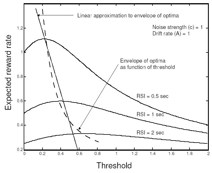
Fig. 2 shows the expected reward rate given by Eq. 10 as a function of threshold z for various values of RSI (Fig. 2A), noise (c; Fig. 2B) and drift rate (A; Fig. 2C) (Bogacz et al.., in review). For all values of RSI, noise and drift, this function is smooth and has a unique maximum, indicating that there is a single optimal threshold for maximizing reward rate, and that a gradient ascent algorithm can be used to find this optimum (although this approach faces some problems that we will consider below).
Figure 2.
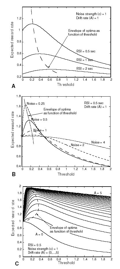
A: Expected reward rate as a function of threshold for three different RSI conditions, with noise and drift held constant; B: Expected reward rate for several noise values, with RSI and drift held constant; C: Expected reward rate for a range of drift values with RSI and noise held constant.
In each plot, a broken line connects the peaks of the reward rate curves, showing the reward rate and corresponding thresholds associated with optimal performance for different values of the DDM parameters (the ‘envelope of the optima’ in Fig. 2). Thus, any mechanism that seeks to optimize reward rate for this decision process must be able to adapt its threshold to the values indicated in the plots in response to changes in task variables.
There is empirical evidence that human participants, performing well-practiced tasks, are capable of such adaptation over relatively short intervals (e.g., in as few as 5–10 trials) following a change in task conditions (Bogacz et al., in review; Ratcliff, VanZandt & McKoon, 1999). Several theories have been proposed for how such adaptations may occur (e.g., Busemeyer & Myung, 1992; Erev, 1998; Myung & Busemeyer, 1989). However, these have typically been described in terms of discrete updating algorithms (for an example, see Table 1). While such algorithms provide a useful abstract specification of the component processes required for threshold adaptation, several challenges arise when considering how they may be implemented.
Table 1.
Hill-climbing algorithm for threshold adaptation that maximizes reward rate, after Myung & Busemeyer (1989).
| Step | Instruction |
|---|---|
| 1. | estimate the reward rate at an initial threshold |
| 2. | randomly take a step upward or downward in threshold value |
| 3. | estimate the reward rate at the new threshold |
| 4. | compute the difference in reward rate estimates |
| 5. | divide the difference by the size (or sign) of the change in threshold value to get an estimate of the gradient of the reward rate curve |
| 6. | if the estimated slope is positive, take another step in threshold value in the same direction; else take a step in the opposite direction; go to (3) and repeat. |
First, any reasonable reward rate estimation process takes time, but algorithms like that in Table 1 assume that threshold changes are made at discrete intervals. It is therefore undetermined how long the system should wait at a given threshold in order to develop a reasonable estimate of the associated reward rate before making a modification: with too few trials the estimate will be poor; with too many, convergence will be slow. Second, there is the question of step-size selection: step sizes that are too large cause oscillation of the threshold around the optimum value; step sizes that are too small again cause slow convergence. This problem can be addressed by introducing additional mechanisms that progressively reduce the step size, but this adds complexity to the model. These algorithms also typically require a memory of old reward rate values, and a means to compare new and old values in order to compute gradients. In the sections that follow, we describe a neural network model that addresses these issues. The model operates in continuous time, requires no explicit value comparison mechanisms, and achieves rapid and stable adaptation to threshold values that approximate the optimal reward rate.
We begin by describing an implementation of a neural network mechanism for detecting threshold-crossing. We then describe a mechanism for reward estimation. Finally, we demonstrate how the latter can be used to adapt the threshold mechanism in order to maximize reward rate.
4 Thresholds as an affine function of reward rate
The threshold in the DDM is a step function applied to the accumulated evidence (for evidence less than the threshold, the output is 0; for evidence greater than the threshold, the output is 1). In order to implement such a crisp function in a neural network, a McCulloch-Pitts neuron (McCulloch & Pitts, 1943) can be used, or an approximation based on a sigmoid unit with strong gain (see Fig. 3A). Inputs that fall below the inflection point of the curve will fail to activate the unit, while those that fall above it will activate the unit maximally. The effective threshold can be manipulated by providing a constant input (or bias) to the unit, with a positive bias in effect shifting the function to the left (decreasing the threshold), and a negative bias shifting it to the right (increasing the threshold).
Figure 3.
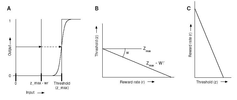
A: Thresholds can be implemented by a simple step-function, or McCulloch-Pitts neuron (McCulloch & Pitts, 1943), which in turn can be approximated by a sigmoid with strong gain. A threshold can be reduced from zmax to zmax − wr by giving the unit additional excitation wr, representing weighted reward rate, so that evidence need only be accumulated to this level to produce a response; B: Threshold represented as a linear function of reward rate; C: By exchanging the vertical and horizontal axes, this prescription for threshold setting based on reward rate can be compared to the predicted reward rate as a function of threshold.
In our model, subthreshold levels of excitation provided to threshold units from non-evidence-accumulating units will act to reduce the effective threshold with respect to the accumulators. An input x > 0, scaled by a positive synaptic weight w, reduces the effective threshold by wx. Thus, if a level zmax of evidence is required for threshold crossing in the absence of additional excitation, the level drops to zmax −wx. This defines an affine function of x (a linear transformation plus a constant): precisely the transformation required by the abstract threshold adaptation algorithm described in section 6. Accordingly, our algorithm may be implemented by connecting one or more additional units to the threshold detectors with appropriate synaptic weights w and by setting the bias (γ in Eq. 5) of the threshold detectors to zmax (see Fig. 9). We shall further discuss implementation, and possible neural substrates, in sections 6–7.
Figure 9.
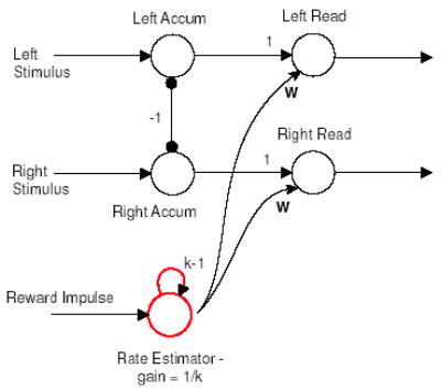
A five-unit neural network that implements the decision mechanism. Mutually inhibiting accumulator units in the first layer approximate a DDM, units with high gain and bias in the second layer detect theshold crossings, and a reward rate estimator with balanced feedback and gain modulates the detector thresholds according to z = zmax − wr.
5 Estimating reward rate
The threshold adaptation algorithm to be described in section 6 seeks to optimize performance in the TAFC task by using a running estimate of the current reward rate to modulate behavior. Here we show how that estimate of reward rate can be computed by a linear filter or ‘leaky integrator’ that is incremented in response to reward impulses s(t) while decaying continuously over time (as in, e.g., Sugrue, Corrado & Newsome, 2004a). The estimate, r(t), evolves according to:
| (11) |
Thus, r(t) at a given time is an exponentially-weighted time-average of the instantaneous reward signal s(t) in which the time constant k determines the speed of adaptation to changes in s(t). Following a step change, r(t) approaches s(t) exponentially at rate 1/k. More generally, large values of k attenuate high frequency fluctuations in s(t) (Oppenheim & Willsky, 1996). Discrete rewards can be modeled in continuous time as a sequence of narrow pulses or Dirac-delta impulses (see Fig. 4), in which case r(t) will approach the steady state mean of the reward rate.
Figure 4.
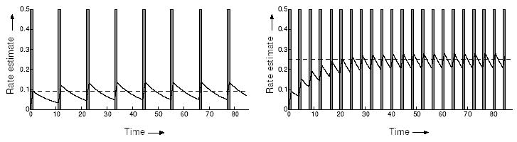
Reward rate estimate r(t) (sawtooth curve) in response to a sequence of short reward pulses s(t) (gray rectangles). Here the rewards are pulses of height 1 and width 1. In both cases the estimated reward rate oscillates around its true frequency, shown by the dotted line. Left panel: slow pulse rate; Right panel: fast pulse rate.
Eq. 11 computes a continuous version of the time-discounted averaging usually seen in discrete-time reinforcement learning algorithms (cf. Doya, 2000). The averaging of Eq. 11 may be computed exactly by a linearized connectionist unit (Eq. 5) in which recurrent self-excitation of strength k − 1 is balanced against an activation function of slope 1/k, as can be seen by simple algebra:
| (12) |
A single unit can therefore compute the reward rate estimate required by the threshold adaptation algorithm. The use of a sigmoid rather than a linear activation function would make the relationship of Eq. 12 to Eq. 11 approximate rather than exact.
6 Threshold adaptation algorithm
We are now in a position to describe an algorithm that builds on the DDM of Eq. 1 and the reward rate estimator of Eq. 11 by modeling threshold as an affine function of a continuously evolving reward rate estimate, as suggested in section 4. This is implemented in a neural network by exciting the threshold detector of Fig. 3 in proportion to the reward rate estimate. The resulting system has an attractor near the optimal threshold across a range of RSI conditions, and its large domain of attraction makes it robust to noise in reward rate estimates and in the activation of threshold and accumulator units.
6.1 Discrete time description
The algorithm proposed below can be understood most easily by first considering the discrete-time version illustrated in Fig. 5. Suppose one starts with an arbitrary threshold value, Thresh1, as in Fig. 5A. The appropriate curve from Fig. 2 specifies the expected reward rate RR1 at that threshold value. After the first trial, Thresh1 is updated in response to a new estimate of the reward rate (based on how long the trial took and whether it produced a reward or not) by mapping RR1 to Thresh2 by the affine transformation. The process is repeated to compute RR2, Thresh3, etc., and progress can be traced by a staircase or ‘cobweb diagram’ (cf. Jordan & Smith, 1999), as indicated in Fig. 5B. Given the unimodal shape of the expected reward rate function and the slope of the transformation line, rapid convergence to their unique intersection occurs, and we note that step sizes adapt automatically, as shown by the decreasing width of the staircase in Fig. 5B as the intersection is approached.
Figure 5.
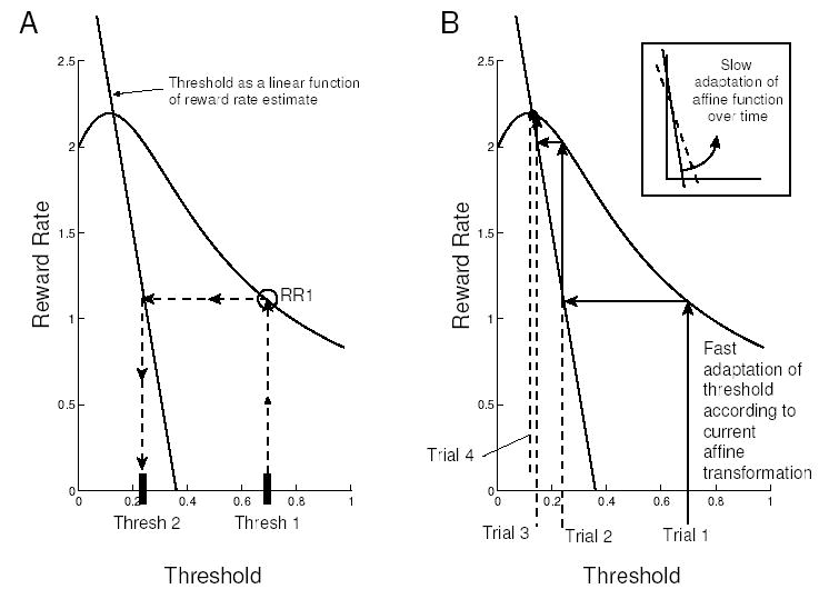
A: Threshold selection after a single trial of the discrete-time description of the algorithm; B: Convergence to nearly optimal threshold after 4 trials.
To obtain near-optimal performance, the transformation line must intersect the reward rate curve at or near its apex. Further on, we suggest that this line can be chosen to approximate the relationship between threshold and optimal reward rate over a range of task parameters (see Fig. 6), and that this line itself may be subject to adaptation over longer time scales.
Figure 6.
The affine function that translates reward rate estimates into threshold produces the best performance when it approximates the envelope of optima (dashed curve), because it intersects the expected reward rate curves near their peaks for a range of RSI conditions. Different ranges of RSI conditions require different affine approximations, and the function is assumed to adapt slowly in response to RSI conditions experienced over a longer time scale.
6.2 Continuous time system
We define the continuous time system as a set of SDEs augmented by conditions for threshold crossing and decision variable resetting:
| (13) |
| (14) |
| (15) |
| (16) |
| (17) |
| (18) |
| (19) |
Here x (Eqs. 13–14) is the decision variable in the DDM, r in Eq. 15 is the running estimate of reward rate, and z in Eq. 16 is the threshold. Eqs. 13, 14 and 19 model the effects of RSI (which impacts reward rate) as well as the assumption that the decision variable starts at the origin on each new trial.1 Specifically, when a stimulus is present, the RSI variable is set to 0 (Eq. 19) and first-passage of the decision variable x beyond either threshold ±z is taken as the time of decision, τ (Eq. 18). At this point, Eq. 19 specifies the response-stimulus interval RSImax for the next trial, and Eq. 13 resets the decision variable to 0. For correct responses, Eqs. 15 and 17 apply a Dirac-delta impulse to the reward rate estimator, which otherwise decays exponentially (see Fig. 4). The threshold z is determined entirely by the reward rate estimate r via the affine function of Eq. 16. In Section 6.4 we show that the continuous system (Eqs. 13–19) shares the property of rapid convergence to near-optimal thresholds of its discrete time version.
6.3 Robustness, generality and parsimony
Given the affine function z = zmax − wr relating threshold to reward rate, the continuous system (Eqs. 13–19) accomplishes gradient ascent without explicit memory, reward-rate comparison or step-size reduction mechanisms. It is also robust to estimation errors and noise, since the intersection point of Fig. 5 is a global attractor. Furthermore, it can be used to adapt the threshold to its optimal value across a range of task parameters. As noted earlier, behavioral evidence suggests that human participants, performing well-practiced tasks, are capable of adaptation over as few as 5–10 trials following a change in task conditions (Bogacz et al, in review; Ratcliff, VanZandt & McKoon, 1999).
The method’s performance depends on the slope w and intercept zmax of the affine function. This function defines a parsimonious linear approximation of the relationship between the optimal threshold and reward rate across a range of task conditions, as in Fig. 2, provided that the resulting line passes close to the reward rate maxima indicated by the dashed curve of Fig. 6.2 We shall assume that these parameters have been learned, for a given task, through practice under different trial conditions (e.g., RSI or noise level). In Section 6.5 we indicate how this can be done by reinforcement learning. First we demonstrate that, like the discrete time version of the algorithm described in section 6.1, the continuous system (Eqs. 13–19) rapidly convergences to near-optimal thresholds.
6.4 Simulations
Numerical simulations of the continuous-time algorithm demonstrate its effect on the behavioral variables of interest: response time and accuracy. According to an optimal analysis of the DDM in this task, thresholds should be set lower for faster RSI conditions, producing faster mean RT and higher error rates. Fig. 7 shows representative timecourses of the decision process variables for one parameterization of the abstract diffusion model in Eqs. 13–19, along with the optimal thresholds and associated reward rates before and after a task condition switch. Note how the system updates from arbitrary initial conditions and again following the switch.
The right panel of Fig. 8 shows RT distributions and error rates for the model of Eqs. 13–19, illustrating a speed-accuracy tradeoff similar to tradeoffs seen in human behavioral data (left panel, from a pilot study we conducted). In each panel, median and interquartile RTs are shown on the left and error rates on the right. These demonstrate significantly faster RTs for shorter RSIs (Wilcoxon rank-sum test, p < 0.01, each pairwise comparison), and also significantly higher error rates for shorter RSIs (pairwise t-test, p < 0.001).
Figure 8.
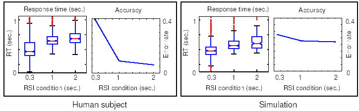
Speed-accuracy tradeoffs produced by a human subject (left panel) and by the algorithm (right panel). The horizontal axis in all plots represents the RSI condition for blocks of trials (0.3, 1 or 2 seconds). Left plot in each panel shows a boxplot of RT, with median RT represented by the middle notch, interquartile RT range (25th–75th percentile) denoted by height of box, and outliers denoted by whiskers. Right plots in each panel show corresponding error rates.
Finally, Fig. 9 shows the neural implementation of the abstract model (in which a single decision variable and threshold are decomposed into two accumulators and two threshold units), and Fig. 10 shows activation timecourses of its units in response to changing RSI conditions. As pointed out in section 4, the slope w of the affine function (Fig. 3B) corresponds to the connection weight from the reward rate estimator to the thresholding units, and the intercept zmax can be interpreted as the bias (γ) of the sigmoid (Eq. 5), or as an additional input.
Figure 10.
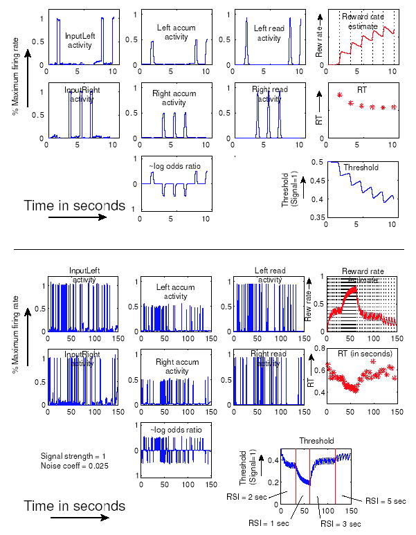
Activations of all units in the network of Fig. 9 are plotted, the position of each plot corresponding to the position of each unit in the circuit diagram. The top set of panels shows a short timecourse, and the bottom set a longer one that illustrates fast threshold adaptation. First column shows inputs to left and right channels. Second column plots left and right accumulator activations and the log odds ratio of evidence derived from their difference. Third column shows left and right threshold detectors. Top plot in the fourth column shows the reward rate monitor, with dotted vertical lines marking stimulus onsets, showing that RSI was decreased from 2 to 1 sec at about 30 secs, and increased from 1 to 3 secs at about 60 secs. Response time (RT) is plotted below as asterisks. Note the similarity between the rate monitor activity and the plots of threshold at bottom right.
6.5 Learning the critical parameters
The model we have described thus far assumes a linear approximation of the relationship between optimal threshold and reward rate. However, the best approximation differs considerably across different ranges of task parameters (see Fig. 6). Here we consider the possibility that this approximation - the affine function used to adapt the threshold - can itself be adapted through learning. To achieve this, reward rates must be experienced for different values of task parameters, such as RSI and stimulus discriminability.
Noting that the reward rate of Eq. 10 depends on signal-to-noise ratio A/c, threshold-to-signal ratio z/A, and RSI in a complex, nonlinear manner, it is clear that the slope and intercept parameters w and zmax represent a substantial compression of information. However, this is useful only insofar as the affine function z = zmax −wr (shown as the straight lines in Figs. 5 and 6) reasonably approximates the envelope of reward rate optima (shown as the dashed curves in Figs. 2 and 6) over a given range of task conditions. For example, the best linear approximation for 500 msec – 1 sec RSIs would significantly differ from the one for 1 – 2 sec values (see Fig. 6). Since linearizations may provide good approximations only over limited ranges of task parameters, it seems reasonable to assume that the approximation given by the affine function may be tuned to accommodate different task environments. This can be accomplished by generic reinforcement learning.
Our arguments supporting fast threshold convergence assume an affine function that is fixed or that changes slowly in comparison to reward rate estimates. The affine function effectively exploits knowledge about the shape of the reward rate curves, trading off generality for speed and task-specificity. Learning the transformation requires exploration of a larger space of possibilities. We therefore propose that such ‘environmental models’ are learned on a slow time scale, and then used as described above to make rapid improvements to task performance in ‘sub-environments.’
As an alternative to adapting the linear approximation, reinforcement learning could be applied directly to threshold adjustment itself. That is, reinforcement learning could be used to produce a full representation of the multi-parameter family of non-linear relationships between thresholds and reward rates. Nevertheless, as with simple hill-climbing, general reinforcement learning methods would still require annealing or step-size reduction schedules tuned to these relationships (cf. Section 3) in order to adapt thresholds quickly to a train of incoming rewards, while simultaneously settling securely on good parameter values in the face of noise (this is another instance of a stability/plasticity tradeoff; Grossberg, 1987). Separating the time scales allows us to obtain the best of both worlds in this task by applying the threshold update algorithm over a time scale of 5–10 trials while simultaneously using reinforcement learning in the background to adjust slope and intercept parameters over a time scale spanning multiple blocks of trials.
In work referred to in Simen et al. (2005) and to be described in a future publication, we have shown that parameters such as slope and intercept can be learned by continuous-time versions of temporal difference algorithms such as the actor-critic method (cf. Doya, 2000). The proposed method draws on the stochastic real-valued unit algorithm of Gullapalli (1990), and is closely related to the Alopex algorithm of Harth & Tzanakou (1976) and a general class of stochastic optimization algorithms (see Kushner & Yin, 1998). Specifically, connection weights from the reward rate estimator to the threshold units of Fig. 9, which correspond to slope, can be updated as in Eq. 15 of section 6.2, but at a much slower rate (larger k), and to obtain the correct hill-climbing behavior, the input (−r(t) + R(t)) in Eq. 15 can be replaced by a product of the derivatives of longer-term averages of reward rate and of the weight itself. Thus, slopes are adjusted only when reward rates are consistently rising or falling, as they would, for example, following a significant change of RSI range. We show that chains of first order units can approximate derivatives, and also suggest a biologically-plausible neural substrate that employs dopamine modulation of glutamatergic synapses in cortico-striatal circuits.
7 Discussion
We have demonstrated that very simple neural mechanisms can give rise to speed-accuracy tradeoffs that maximize reward rate and that are similar to the tradeoffs exhibited by human subjects. Our approach exploits attractor dynamics to deal with the challenges faced by straightforward reinforcement learning and gradient ascent approaches to the threshold adaptation problem, as well as more abstract algorithms (e.g., Busemeyer & Myung, 1992; Erev & Barron, 2005). The model we describe operates in continuous time, is able to reliably estimate reward rate, rapidly and stably converges on a threshold that optimizes reward rate to a reasonable approximation, and does not require any additional apparatus for explicitly remembering or comparing previous estimates of reward rate with current estimates.
A critical feature of the model is that it relies on a linear approximation of the relationship between optimal threshold and reward rate across a range of task conditions. This serves two purposes. First, it provides a representation of this relationship that is considerably simpler than the actual curvilinear relationship (shown in Fig. 7.2) which is itself the solution to a transcendental equation that can only be approximated numerically (Bogacz et al., in review). Second, and perhaps more importantly, it allows the neural implementation of a threshold adaptation algorithm that uses an affine function to achieve rapid convergence to a threshold in close proximity to the optimal one. However, this use of a linear approximation also represents a potential limitation of the model, insofar as the specific best approximation varies as a function of task parameters (see Fig. 6). We have suggested how the parameters defining the linear approximation could themselves be adapted using simple principles of reinforcement learning, although this adaptation would need to occur on a significantly longer time scale than that of threshold adaptation. The effects of these simultaneous adaptations at different times scales, and their relationship to observations about human performance, remain to be explored in future theoretical and empirical studies.
Previous non-neural modeling work has approached the issue of speed-accuracy tradeoffs from the perspective that subjects try to minimize a cost consisting of a linear combination of speed and accuracy, subject to information processing constraints (e.g., Maddox & Bohil, 1998; Mozer, Colagrosso & Huber, 2000). This approach seems entirely consistent with an extended version of our model that also maintains an estimate of error rate in the same manner as it estimates reward rate. What is new here is the implementation of these processes using neurally plausible mechanisms and a dynamical systems analysis of how and why they work. Reward rate estimators, by directly exciting threshold readout units, can implement a speed-accuracy tradeoff that is nearly optimal across a range of task conditions.
In this respect, our approach is similar to an existing neural model in which continuous feedback in the form of motivational signals influences underlying decision making circuits based on lateral inhibition (‘gated dipoles’) in order to change their stimulus sensitivity (Grossberg, 1982). To the best of our knowledge, however, that type of model has not been applied specifically to the problem of estimating and responding to the rate of reward in a free response task.
It is also worth noting the similarity of the reward rate estimate discussed in section 5 to an ‘accumulating’ eligibility trace as used in reinforcement learning (Sutton & Barto, 1998). The two quantities are computed in the same way, but the purpose of the eligibility trace is typically for changing weights in reinforcement learning, whereas in our case we simply feed the equivalent quantity into the response units as an additional input. In this way, our approach corresponds to an activation-based mechanism, whereas the traditional use of an eligibility trace (as applied to brain modeling) is for governing synaptic plasticity. Combining both approaches should provide a means for optimizing performance at both short and long time scales.
7.1 Implementation in the brain
Recent findings suggest that the components of our model may reflect the operation of specific neural structures. Previous reports have suggested that areas of LIP as well as the frontal eye field may correspond to the accumulators in the DDM (e.g., Gold & Shadlen, 2001; Hanes & Schall, 1996; Shadlen & Newsome, 2001). Other findings have begun to identify neural mechanisms that may be involved in reward rate estimation and the adaptation of decision parameters. For example, given the role of orbitofrontal cortex (OFC) in encoding the reward value of objects or actions (e.g., Rolls, 2000) and evidence that it may also encode the rate of reward (Sugrue, Corrado & Newsome, 2004b), it is possible that the reward rate estimator unit in Fig. 9 may serve as a simple, first-order approximation to OFC function in the type of decision making task discussed here.
Further, activity in areas of monkey parietal cortex thought to be involved in sensorimotor transformation has been shown to be sensitive to expected future reward (Platt & Glimcher, 1999) and the relative values of competing choices (Sugrue et al., 2004a) in occulomotor tasks. Similar effects have been observed in other brain areas thought to be involved in the decision-making process, such as the dorsolateral prefrontal cortex (Barraclough, Conroy & Lee, 2004; Leon & Shadlen, 1999). Thus it is possible that connections from OFC to threshold detectors implemented in frontal and/or parietal cortex may implement something like our threshold adaptation algorithm.
Given their role in reward processing, the basal ganglia are also promising candidates for involvement in threshold modulation. Along these lines, Frank (2006) discusses a pattern of anatomic connections and a possible role for the subthalamic nucleus (STN) that are consistent with the mechanisms we have described. There, the proposed role of the STN is effectively to increase the threshold when increased conflict is detected between competing responses in a Go/No-Go task. In this way, emphasis shifts toward accuracy and away from speed when response conflict is high. A shift in the opposite direction in response to reward rate might similarly be achieved by connections from OFC to the striatum, given the role that the striatum plays in promoting, rather than inhibiting, the propagation of activity through the basal ganglia (as the STN does).
Our model assumes that speed-accuracy tradeoffs are implemented in the brain at a single stage of processing (the threshold-crossing detection stage) through modulation by an estimate of reward rate. However, neither reward rate estimation nor threshold-crossing detection are functions that are likely to be discretely localized in the brain. As we have noted above, many areas of the brain are sensitive to information about reward. Furthermore, the specific neural mechanisms responsible for information accumulation and threshold adjustment are likely to vary based on the demands of a given task (e.g., whether it involves visual or auditory information, and a manual or occulomotor response). Presumably these are selected by frontal control mechanisms for task engagement (e.g., Miller & Cohen, 2001). We propose, however, that our model identifies fundamental principles of operation that may be shared in common by the neural mechanisms involved in decision making across different processing domains. Along these lines, it will be important to explore the relationship between these mechanisms and others that have been proposed for the adaptive regulation of performance. This includes the use of processing conflict to adapt threshold as well as attentional variables (e.g., Botvinick et al., 2001), as well as the role of neuromodulatory mechanisms in adapting processing parameters such as threshold and gain (e.g., Aston-Jones & Cohen, 2005).
7.2 Extensions to a broader range of decision tasks
Our model has focused exclusively on free responding in the TAFC task. However, the basic ideas should extend to address a broader range of more realistic tasks. For example, it should be straightforward to incorporate our reward rate estimation and threshold adaptation mechanisms into models for free responding in multi-alternative decision tasks (e.g., Bogacz & Gurney, in review; McMillen & Holmes, 2006; Usher & McClelland, 2001), as well as Go/No-Go tasks as discussed above. It should also be possible to address other response conditions, such as deadlining, by elaborating the model to maintain an estimate of late-response rate, and to use this in place of reward rate estimates to set an internal deadline for responding. Finally, decision making tasks that also involve working memory over a delay period can be modeled by implementing thresholds via detector units with strong, self-excitatory positive feedback - as in the firing rate models of Nakahara & Doya (1998) and Simen (2004) and the spiking model of Wang (2002) - rather than non-self-exciting units with very steep gain in their activation functions (as in section 4). The analysis presented here in terms of units with activation functions that are step functions carries over without loss of generality to such self-exciting units (Simen, 2004).
We hope that this model helps extend the foundation that has begun to develop for formalizing decision-making tasks, particularly those that integrate continuous time reward monitoring and prediction with sensory mechanisms, and that it may serve as a bridge between psychological function and neural implementation.
Figure 1.
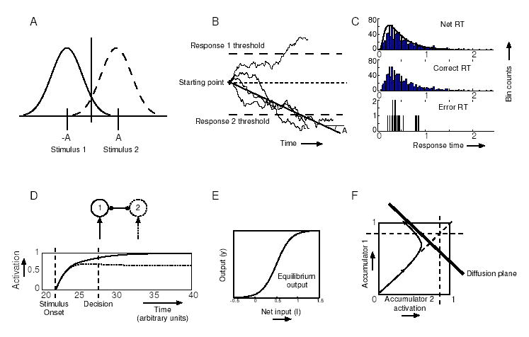
A: The two stimulus distributions; B: Sample paths of a drift-diffusion process; C: Long-tailed analytical RT density (solid curve) and simulated RT histogram (top), correct RT histogram (middle), error RT histogram (bottom); D: Time courses of noise-free, mutually inhibitory evidence accumulation units with sigmoid activation functions; E: The sigmoid activation function; F: A smoothed sample path of mutually inhibitory accumulator activations in the (y1, y2)-phase space showing rapid attraction to a line (the ‘diffusion plane’) followed by drift and diffusion in its neighborhood.
Acknowledgments
This work was supported by PHS grants MH58480 and MH62196 (Cognitive and Neural Mechanisms of Conflict and Control, Silvio M. Conte Center) (PS, JDC and PH) and DoE grant DE-FG02-95ER25238 (PH).
Footnotes
Patrick Simen
phone: 609-258-6155
FAX: 609-258-1735
email: psimen@math.princeton.edu
Jonathan D. Cohen
phone: 609-258-2696
FAX: 609-258-2574
email: jdc@princeton.edu
Philip Holmes
phone: 609-258-2958
FAX: 609-258-1735
email: pholmes@Math.Princeton.EDU
This last, rather unrealistic assumption implies a discontinuous decision variable trajectory over time, but it can be relaxed without loss of generality by introducing a refractory period and modeling the system as a stable, rapidly decaying Ornstein-Uhlenbeck process during the RSI, as done in Fig. 7; we use the simpler system here for ease of discussion.
Ideally one would use the envelope of optima - the dashed curve - to transform reward rate estimates into thresholds, but we are constrained to linearity by the plausible neural mechanism assumed in section 4: superposition of synaptic inputs to the threshold units.
References
- Aston-Jones G, Cohen JD. An integrative theory of locus coeruleus-norepinephrine function: adaptive gain and optimal performance. Annual Review of Neuroscience. 2005;28:403–450. doi: 10.1146/annurev.neuro.28.061604.135709. [DOI] [PubMed] [Google Scholar]
- Barraclough DJ, Conroy ML, Lee D. Prefrontal cortex and decision making in a mixed-strategy game. Nature Neuroscience. 2004;7:404–410. doi: 10.1038/nn1209. [DOI] [PubMed] [Google Scholar]
- Bogacz R, Brown E, Moehlis E, Holmes P, Cohen JD. The physics of optimal decision making: a formal analysis of models of performance in two-alternative forced choice tasks. doi: 10.1037/0033-295X.113.4.700. (in review) [DOI] [PubMed] [Google Scholar]
- Botvinick MM, Braver TS, Barch DM, Carter CC, Cohen JD. Conflict monitoring and cognitive control. Psychological Review. 2001;108(3):624–652. doi: 10.1037/0033-295x.108.3.624. [DOI] [PubMed] [Google Scholar]
- Brody CD, Hernandez A, Zainos A, Romo R. Timing and neural encoding of somatosensory parametric working memory in macaque prefrontal cortex. Cerebral Cortex. 2003;13:1196–1207. doi: 10.1093/cercor/bhg100. [DOI] [PubMed] [Google Scholar]
- Brown E, Gao J, Holmes P, Bogacz R, Gilzenrat M, Cohen JD. Simple neural networks that optimize decisions. International Journal of Bifurcation and Chaos. 2005;15 (3):803–826. [Google Scholar]
- Busemeyer JR, Myung IJ. An adaptive approach to human decision making: learning theory and human performance. Journal of Experimental Psychology: General. 1992;121:177–194. [Google Scholar]
- Busemeyer JR, Townsend JT. Decision field theory: A dynamic-cognitive approach to decision making in uncertain environments. Psychological Review. 1993;100:432–459. doi: 10.1037/0033-295x.100.3.432. [DOI] [PubMed] [Google Scholar]
- Cohen M, Grossberg S. Absolute stability of global pattern formation and parallel memory storage by competitive neural networks. IEEE Transactions on Systems, Man and Cybernetics. 1983;13:815–826. [Google Scholar]
- Doya K. Reinforcement learning in continuous time and space. Neural Computation. 2000;12:219–245. doi: 10.1162/089976600300015961. [DOI] [PubMed] [Google Scholar]
- Erev I. Signal detection by human observers: a cut-off reinforcement learning model of categorization decisions under uncertainty. Psychological Review. 1998;105:280–298. doi: 10.1037/0033-295x.105.2.280. [DOI] [PubMed] [Google Scholar]
- Erev I, Barron G. On adaptation, maximization, and reinforcement learning among cognitive strategies. Psychological Review. 2005;112:912–931. doi: 10.1037/0033-295X.112.4.912. [DOI] [PubMed] [Google Scholar]
- Frank M. Hold your horses: a dynamic computational role for the subthalamic nucleus in decision making. Neural Networks. 2006 doi: 10.1016/j.neunet.2006.03.006. this issue. [DOI] [PubMed] [Google Scholar]
- Freeman WJ. Nonlinear gain mediating cortical stimulus-response relations. Biological Cybernetics. 1979;33:237–247. doi: 10.1007/BF00337412. [DOI] [PubMed] [Google Scholar]
- Gardiner CW. Handbook of Stochastic Methods. 2nd Ed. New York: Springer; 1985. [Google Scholar]
- Gold JI, Shadlen MN. Representation of a perceptual decision in developing oculomotor commands. Nature. 2000;404:390–394. doi: 10.1038/35006062. [DOI] [PubMed] [Google Scholar]
- Gold JI, Shadlen MN. Neural computations that underlie decisions about sensory stimuli. Trends in Cognitive Sciences. 2001;5:10–16. doi: 10.1016/s1364-6613(00)01567-9. [DOI] [PubMed] [Google Scholar]
- Gold JI, Shadlen MN. Banburismus and the brain: Decoding the relationship between sensory stimuli, decisions and reward. Neuron. 2002;36:299–308. doi: 10.1016/s0896-6273(02)00971-6. [DOI] [PubMed] [Google Scholar]
- Grossberg S. A psychophysiological theory of reinforcement, drive, motivation and attention. Journal of Theoretical Neurobiology. 1982;1:286–369. [Google Scholar]
- Grossberg S. Competitive learning: from interactive activation to adaptive resonance. Cognitive Science. 1987;11:23–63. [Google Scholar]
- Grossberg S, Gutowski W. Neural dynamics of decision making under risk: affective balance and cognitive-emotional interactions. Psychological Review. 1987;94(3):300–318. [PubMed] [Google Scholar]
- Guckenheimer J, Holmes P. Nonlinear oscillations, dynamical systems, and bifurcations of vector fields. Springer-Verlag; 1983. [Google Scholar]
- Hanes DP, Schall JD. Neural control of voluntary movement initiation. Science. 1996;274:427–430. doi: 10.1126/science.274.5286.427. [DOI] [PubMed] [Google Scholar]
- Harth E, Tzanakou E. Alopex: A stochastic method for determining visual receptive fields. Vision Research. 1974;14:1475–1482. doi: 10.1016/0042-6989(74)90024-8. [DOI] [PubMed] [Google Scholar]
- Holmes P, Brown E, Moehlis J, Bogacz R, Gao J, Aston-Jones G, Clayton E, Rajkowski J, Cohen JD. Optimal decisions: From neural spikes, through stochastic differential equations, to behavior. IEICE Transactions on Fundamentals on Electronics, Communications and Computer Sciences. 2005;88(10):2496–2503. [Google Scholar]
- Jordan DW, Smith P. Nonlinear Ordinary Differential Equations. 3rd edition Oxford University Press; New York, NY: 1999. [Google Scholar]
- Kushner HJ, Yin GG. Stoachastic approximation algorithms and applications. New York; Springer: 1997. [Google Scholar]
- Laming DRJ. Information theory of choice reaction time. New York: Wiley; 1968. [Google Scholar]
- Leon MI, Shadlen MN. Effect of expected reward magnitude on the response of neurons in the dorsolateral prefrontal cortex of the macaque. Neuron. 1999;24:415–425. doi: 10.1016/s0896-6273(00)80854-5. [DOI] [PubMed] [Google Scholar]
- Luce RD. Response times: their role in inferring elementary mental organization. New York: Oxford University Press; 1986. [Google Scholar]
- Maddox WT, Bohil CJ. Base-rate and payoff effects in multidimensional perceptual categorization. Journal of Experimental Psychology: Learning, Memory and Cognition. 1998;24:1459–1482. doi: 10.1037//0278-7393.24.6.1459. [DOI] [PubMed] [Google Scholar]
- McCulloch W, Pitts W. A logical calculus of the ideas immanent in nervous activity. Bulletin of Mathematical Biophysics. 1943;5:115–133. [PubMed] [Google Scholar]
- McMillen T, Holmes P. The dynamics of choice among multiple alternatives. Journal of Mathematical Psychology. 2006;50:30–57. [Google Scholar]
- Miller EK, Cohen JD. Integrative theory of PFC function. Annual Review of Neuroscience. 2001;24:167–202. doi: 10.1146/annurev.neuro.24.1.167. [DOI] [PubMed] [Google Scholar]
- Mozer MC, Colagrosso MD, Huber DH. A rational analysis of cognitive control in a speeded discrimination task. In: Dietterich T, Becker S, Ghahramani Z, editors. Advances in Neural Information Processing Systems 14. Cambridge, MA: MIT Press; 2002. pp. 51–57. [Google Scholar]
- Myung IJ, Busemeyer JR. Criterion learning in a deferred decision making task. American Journal of Psychology. 1989;102:1–16. [Google Scholar]
- Nakahara H, Doya K. Dynamics of attention as near saddle-node bifurcation behavior. In: Touretzky DS, Mozer MC, Hasselmo ME, editors. Advances in Neural Information Processing Systems 8. MIT Press; 1996. pp. 38–44. [Google Scholar]
- Oppenheim AV, Willsky AS. Signals and Systems. 2nd edition. New York: Prentice Hall; 1996. [Google Scholar]
- Palmer J, Huk AC, Shadlen MN. The effect of stimulus strength on the speed and accuracy of a perceptual decision. Journal of Vision. 2005;5(5):376–404. doi: 10.1167/5.5.1. [DOI] [PubMed] [Google Scholar]
- Platt ML, Glimcher PW. Neural correlates of decision variables in parietal cortex. Nature. 1999;400:233–238. doi: 10.1038/22268. [DOI] [PubMed] [Google Scholar]
- Ratcliff R. A theory of memory retrieval. Psychological Review. 1978;85:59–108. [Google Scholar]
- Ratcliff R, Rouder JN. Modeling response times for two-choice decisions. Psychological Science. 1998;9:347–356. [Google Scholar]
- Ratcliff R, Van Zandt T, McKoon G. Connectionist and diffusion models of reaction time. Psychological Review. 1999;106:261–300. doi: 10.1037/0033-295x.106.2.261. [DOI] [PubMed] [Google Scholar]
- Roitman JD, Shadlen MN. Response of neurons in the lateral intraparietal area during a combined visual discrimination reaction time task. Journal of Neuroscience. 2002;22:9475–9489. doi: 10.1523/JNEUROSCI.22-21-09475.2002. [DOI] [PMC free article] [PubMed] [Google Scholar]
- Rolls ET. The orbitofrontal cortex and reward. Cerebral Cortex. 2000;10(3):284–294. doi: 10.1093/cercor/10.3.284. [DOI] [PubMed] [Google Scholar]
- Shadlen M, Newsome W. Neural basis of a perceptual decision the parietal cortex (area LIP) of the rhesus monkey. Journal of Neurophysiology. 2001;86:1916–1936. doi: 10.1152/jn.2001.86.4.1916. [DOI] [PubMed] [Google Scholar]
- Simen P. Neural mechanims of control in complex cognition. University of Michigan; 2004. PhD thesis. [Google Scholar]
- Simen P, Holmes P, Cohen JD. Threshold adaptation in decision making. 2005. Society for Neuroscience abstracts. [Google Scholar]
- Smith PL, Ratcliff R. Psychology and neurobiology of simple decisions. Trends in Neuroscience. 2004;27:161–168. doi: 10.1016/j.tins.2004.01.006. [DOI] [PubMed] [Google Scholar]
- Stone M. Models for choice reaction time. Psychometrika. 1960;25:251–260. [Google Scholar]
- Sugrue LP, Corrado GS, Newsome WT. Matching behavior and the representation of value in the parietal cortex. Science. 2004a;304:1782–1787. doi: 10.1126/science.1094765. [DOI] [PubMed] [Google Scholar]
- Sugrue LP, Corrado GS, Newsome WT. Neural correlates of value in orbitofrontal cortex of the rhesus monkey. Society for Neuroscience abstracts 2004b [Google Scholar]
- Sutton RS, Barto AG. Reinforcement learning. Cambridge, MA: MIT Press; 1998. [Google Scholar]
- Usher M, McClelland J. On the time course of perceptual choice: the leaky competing accumulator model. Psychological Review. 2001;108:550–592. doi: 10.1037/0033-295x.108.3.550. [DOI] [PubMed] [Google Scholar]
- Wald A, Wolfowitz J. Optimum character of the sequential probability ratio test. Annals of Mathematical Statistics. 1948;19:326–339. [Google Scholar]
- Wang X-J. Probabilistic decision making by slow reverberation in cortical circuits. Neuron. 2002;36:955–968. doi: 10.1016/s0896-6273(02)01092-9. [DOI] [PubMed] [Google Scholar]