Determination of Protein Backbone Structures from Residual Dipolar Couplings

Abstract

There are a number of circumstances where a focus on determination of the backbone structure of a protein, as opposed to a complete all-atom structure, may be appropriate. This is particularly the case for structures determined as a part of a structural genomics initiative where computational modeling of many sequentially related structures from the backbone of a single family representative is anticipated. It is, however, also the case where the backbone may be a stepping-stone to more targeted studies of ligand interaction or protein-protein interaction. Here an NMR protocol is described that can produce a backbone structure of a protein without the need for extensive experiments directed at side-chain resonance assignment or collection of structural information on side-chains. The procedure relies primarily on orientational constraints from residual dipolar couplings as opposed to distance constraints from NOEs. Procedures for sample preparation, data acquisition, and data analysis are described, along with examples from application to small target proteins of a structural genomics project.

Introduction

Residual Dipolar Couplings (RDCs) are now widely used as a source of constraints in the structure determination of biomolecules. Several reviews on the subject have appeared (Al-Hashimi and Patel, 2002; Bax et al., 2001; de Alba and Tjandra, 2002; Prestegard et al., 2000; Tolman, 2001; Zhou et al., 1999) and there are numerous examples of application to proteins in the more recent literature (Alexandrescu and Kammerer, 2003; Assfalg et al., 2003; Beraud et al., 2002; Lin et al., 2004; Nair et al., 2003; Ohnishi et al., 2004; Tossavainen et al., 2003; Zheng et al., 2004). However, in the majority of cases, use has been as a supplement to other structural information, rather than a primary source of information. While this is often appropriate, there are cases in which use as a primary source of structural data should be considered. One case arises in the context of the structural genomics initiative (Adams et al., 2003; Chance et al., 2002; Montelione et al., 2000). This initiative set as its goal the production of massive numbers of three dimensional protein structures in an effort to leverage the information flowing from whole genome sequencing efforts of the previous decade (Burley et al., 1999; Norvell and Machalek, 2000). Production of experimental structures for each gene sequenced would obviously be impossible, but production of a sufficient number of structures to populate “fold space” (10,000 structures in ten years) might be possible with adequate attention to automation of existing methodology and development of new methodology for structure determination. With representative structures in each “fold family” computer modeling methods would then be able to build structures for most sequences. However, even with the reduced number of structures to be determined, the methodology developed would have to be efficient.

For NMR, substantial efficiency might be gained by focusing on backbone structures as opposed to structures complete with all side chain atoms. Given the intent to model most structures starting from representative structures that may have as little as 30% sequence identity, a backbone structure for a fold family representative should be adequate. As much as 70% of the side-chains would, after all, be replaced in the course of modeling a new protein. While structural information is obviously limited, backbone structures may have direct application in other areas as well. Drug discovery programs often rely on perturbations of resonances from just backbone atoms to identify ligand-binding sites (Fesik, 1999; Fesik, 2001; Hajduk et al., 2002; Hajduk et al., 1999). Orientational data collected on ^>15N-^>1H pairs of atoms along the backbone is often enough to align elements of protein complexes (Clore and Schwieters, 2003; Dosset et al., 2001; Weaver and Prestegard, 1998). And, a backbone structure, with assignments of resonances from backbone atoms, is potentially a good starting point for a more complete structure determination. These considerations make presentation of backbone structure determination methodology as a part of this volume particularly appropriate.

Focusing on backbone atoms is, unfortunately, not entirely compatible with a traditional NOE-based approach to protein structure. NOEs stem from very short-range interactions; we can easily measure an NOE for a pair of protons at 3Å separation, but at 6Å, the steep 1/r^>6 distance dependence reduces signal by a factor of 64 and nearly eliminates the possibility of observation. Except for β-sheets, atoms in remote parts of a protein backbone seldom come within 6Å of one another. Reliance on RDC data enters at this point. RDCs show orientational dependence in addition to distance dependence, and these orientational dependencies give rise to constraints that are effective in relating remote parts of the backbone, no matter what their separation in space.

In what follows we present a particular strategy that evolved from an attempt to produce protein structures efficiently as a part of a structural genomics project (Adams et al., 2003). This is, of course, not the only such strategy; there are ones that use different sets of RDC data, and ones that use fundamentally different algorithms for the determination of structure (Andrec et al., 2001a; Andrec et al., 2001b; Delaglio et al., 2000; Haliloglu et al., 2003; Rohl and Baker, 2002). The strategy presented here shares some of the philosophy of these other methods, but also has some unique characteristics. One is that it was designed to work with lower levels of ^>13C enrichment; this can lead to significant cost savings in some situations, but it also avoids some of the complexities associated with ^>13C decoupling and the loss of signal due to multiple magnetization transfer pathways. The ability to use simpler pulse sequences and exploit selective pathways compensates for some of the loss in sensitivity with lower levels of labeling. In addition, prior assignment of resonances is not essential; this avoids the need for collection of separate resonance assignment experiments.

In the following we present the basic rationale for converting RDCs into a three-dimensional backbone structure, a set of experiments that have proven useful in acquiring the required data, and step-by-step examples of applications to structural genomics targets. While the presentation centers on efficiency of structural genomics applications (data acquisition takes about one third the time of a complete NOE based structure), many aspects of the procedure should be of more general utility. Efficient collection of the same subsets of RDC data used in structural genomics applications may find application in refinement of structures based on NOE data, and the procedures described for orienting backbones may have application to assembly of subunits into multi-protein complexes.

Origin of RDCs

Residual dipolar couplings arise from the same basic interaction that gives rise to the NOE, namely a through-space dipole-dipole interaction between nuclei that possess magnetic moments. For a pair of weakly coupled spin one-half nuclei this interaction can be represented as in Eq. 1. Here r is the distance between nuclei i and j, γ_i,j are the magnetogyric ratios for the nuclei, μ₀ is the permeability of space, h is Planck's constant, and θ is the angle between the inter-nuclear vector and the magnetic field. For a directly bonded pair of nuclei, r is fixed and θ becomes the primary source of structural information. Clearly, a constraint on θ for every bond vector along a protein backbone would be a powerful determinant of molecular geometry.

$$D_{\mathit{ij}}=-\frac{{\mu }_0{\gamma }_i\gamma {}_{j}h}{{\left(2\pi r\right)}^3}\langle \frac{3{\cos }^2\theta -1}{2}\rangle$$ (1)

The brackets in Eq. 1 denote averaging over the rapid molecular tumbling that occurs in solution. When this tumbling makes the interaction vector sample directions in space isotropically, the interaction averages to zero and no dipole-dipole contributions to splittings are observed. This is why NMR spectroscopists working in solution seldom worry about direct dipole-dipole contributions to their spectra and rely on indirect spin relaxation contributions such as the NOE for structural information. However, the average can be made non-zero by inducing partial alignment of the molecules studied. As long as molecular tumbling remains rapid, a single average interaction that adds to multiplet splittings in coupled spectra results. Alignment is commonly accomplished with the use of aqueous liquid crystal media such as bicelles or filamentous bacteriophage that interact weakly with the molecule of interest to give departures from isotropic sampling by one part in 10³ or 10⁴. A large number of media for inducing alignment now exist, as do paramagnetic tags that aid self-alignment of molecules in high magnetic fields (Barbieri et al., 2002; Wohnert et al., 2003). These are described in recent reviews (Bax et al., 2001; Prestegard et al., 2004; Prestegard and Kishore, 2001).

Partial alignment, unfortunately introduces hidden unknowns into Eq. 1. One must usually characterize the level of alignment, the asymmetry of alignment, and the direction of the principal alignment axes as seen from the point of the molecule under study. The five additional parameters needed can be considered to be three Euler angles to define the alignment axes (α,β,γ), a principal order parameter (S_zz), and an asymmetry parameter (η). Determining these parameters requires that a significant number of RDCs must be measured for each molecular fragment. However, the extra information obtained is also valuable. If fragments are a part of the same rigid structure they must share the same S_zz and η. If they don't, the existence of internal motions is suggested. Also, the alignment axes must coincide if the fragments are oriented so that they properly represent parts of the same rigid molecule. This will be the basis of our structure determination strategy.

Fortunately, RDCs are easily measured. When all units in Eq. 1 are in SI units, D_ij is given in Hz, and corresponds to the dipole-dipole contribution to the splitting of the doublets that would be observed for each member of a weakly coupled pair of spins. When the spins are directly bonded, substantial through-bond (scalar, J_ij) couplings also exist and the observed splitting would be the sum of scalar and dipole-dipole couplings. Hence, RDCs are measured as differences in splittings of partially aligned (J_ij+D_ij) and isotropic (J_ij) spectra.

While there are a number of ways to extract alignment parameters and evaluate fragment geometry (Delaglio et al., 2000; Hus et al., 2000; Schwieters et al., 2003), the procedure used in the protocol presented here rests on recasting Eq. 1 in terms of elements of a 3×3 order matrix, S_kl (see Eq. 2 and (Saupe, 1968)) D_{max ij} is the coupling for a pair of nuclei at a 1.0 Å separation with their internuclear vector along the magnetic field, and cos(θ_k,l) are the direction cosines relating the inter-nuclear vector to the axes (x,y,z) of an arbitrarily chosen molecular fragment frame.

$$D_{\mathit{ij}}=\frac{D_{\max \mathit{ij}}}{r^3}\sum _{k,l}{S}_{\mathit{kl}}\cos \left({\theta }_k\right)\cos \left({\theta }_l\right)$$ (2)

Because the order matrix is traceless and symmetric, only five order matrix elements are independent in the expression for each RDC. For a given trial geometry of a fragment the cos(θ_k,l) are also known, making a set of equations of the form of Eq.2 solvable for any five or more independent RDC measurements. Singular value decomposition can be used to give a best least squares solution for the order parameters (Losonczi et al., 1999). The order parameters can then be used to back-calculate RDCs for comparison to experiment and evaluation of trial geometries for the fragment (Valafar and Prestegard, 2004).

Conversion of RDCs to Structure

The general procedure for converting RDCs to a protein backbone structure begins with the determination of fragment geometries using the program REDCRAFT (REsidual Dipolar Coupling Residue Assembly and Filter Tool) (H. Valafar and J. H. Prestegard, manuscript in preparation, and to be available at http://nmr.secsg.org). This uses the above order matrix evaluation and back-calculation of RDCs to select proper fragment geometries. It also uses a number of other filters for allowed fragment geometry including a Ramachandran space filter and a torsion angle filter that is based on the Karplus equation for three bond scalar couplings. The program begins by first evaluating geometry solutions using incremented sets of ϕ, ψ values for pairs of peptide planes connected by a common alpha carbon. These geometries are ranked based on agreement with RDCs and other filters; then the top choices from the ranked list for one unit are combined with top choices from a sequentially connected second unit by overlaying the C and N terminal peptide planes. Selection of this second unit is usually based on the overlap of the intra residue C_α chemical shift seen for the first residue with the inter residue C_α chemical shift seen for the second residue in HNCA style experiments. The proposed geometries for the new fragment, containing now three peptide planes and two sets of ϕ, ψ angles, are evaluated and ranked for a next round of extension. Ambiguities in selection of a next residue do, of course arise. These can be resolved to some extent by excluding those connections that produce no acceptable matches to experimental RDCs. However, at some point the process terminates because ambiguities are un-resolvable or data needed for connection are missing due to the occurrence of a proline or just lack of observable data. Fragments having five or six C_αcarbons are usually sufficient to proceed with a first round of structure determination.

Coordinates for the structurally defined fragments are next transformed to a common principal alignment frame (PAF). The Euler angles needed to accomplish this can be found from the transformations that diagonalize the order matrix for each fragment. The software package REDCAT, for REsidual Dipolar Coupling Analysis Tool, provides a means of extracting Euler angles (Valafar and Prestegard, 2004). When all fragments are in their common PAF, assembly into a complete structure remains a problem of translation only. There is one caveat; the insensitivity of Eqs. 1 and 2 to a 180° rotation about any principal axis leads to a four-fold degeneracy in possible fragment orientations. This problem is sometimes obviated when fragments are sequentially separated by only one or two residues, but the problem can be more generally solved by considering alignments from RDCs collected in a second medium (Al-Hashimi et al., 2000). When alignment frames for different media differ in nontrivial ways, only one of the four possibilities for relative alignment of fragments will appear in both sets, allowing a definitive choice of orientations.

Translation of fragments to produce a fully assembled structure is accomplished under distance constraints from a small number of inter-fragment NOEs observed in ¹⁵N edited NOE data sets or from expected covalent connections of fragments once they are placed in sequence. This is done manually using common molecular graphics programs to monitor constraint distances while fragments are translated. The number of observable long-range backbone-to-backbone proton NOEs is obviously small due to the relatively long distances found between backbone atoms, but combining NOE constraints with limitations imposed by covalent connection through the small numbers of residues between fragments, and limitations imposed by van der Waals contact, produces adequate numbers of constraints. Minimally, three translational constraints per fragment are needed.

Obtaining constraints from covalent connection requires placement of fragments in proper sequential positions. Data used to do this can come primarily from correlating C_α chemical shifts with amino acid type. The use of C_α shift deviations from random coil values for each amino acid is commonly used to evaluate secondary structure after resonance assignment (Cornilescu et al., 1999; Wishart and Sykes, 1994; Wishart et al., 1992), but in our case local structure, as opposed to resonance assignment, is known for each fragment; here, the process can be reversed to use shift departures from those found for secondary structure (ϕ, ψ) types to identify specific amino acids. This cannot be done with certainty site-by-site, but connected sets of shifts in fragments containing five or more C_α carbons give high probabilities of placement at unique positions in a known protein sequence. This process has been automated in a program called SEASCAPE for SEquential Assignment by Structure and Chemical shift Aided Probability Estimation (Morris et al., 2004). Definitive assignment and further fragment extension can be aided by ¹⁵N-edited TOCSY data. These data are also useful in assignment of H_α chemical shifts for identification of backbone-to-backbone NOE constraints involving H_α protons.

Final assembled structures can be refined by minimization in programs such as XPLOR-NIH under a combination of NOE and RDC constraints (Schwieters et al., 2003). Use of this refinement step is facilitated by having the assembled fragments in their principal alignment frame. Entry of coordinates for pseudo-atoms defining an alignment frame then involves just simple displacements of pseudo atoms along x, y, and z axes. The axial alignment and rhombicity parameters that this program normally uses can be entered from known relationships to order parameters provided by the REDCAT program; the axial alignment parameter, D_a, and the rhombicity parameter, R, are given as ½(D_max• S_zz) and 2/3η respectively.

Hence, we have a complete protocol for structure determination of protein backbones based primarily on RDC data. Five or more pieces of RDC data are collected about a C_α carbon connecting two peptide planes and allowed ϕ and ψ angles are identified based on best fits to the RDC data (this is usually done for data from two different alignment media). Other C_α carbons are connected based on chemical shift overlap in HNCA style spectra, eventually generating fragments of known geometry of 5 or more such carbons. These fragments are placed in sequence using backbone chemical shift data, and the orientations in space of the fragments are determined. NOEs and connectivity restraints allow translation of fragments to form a crude structure, and this structure is minimized under a combination of RDC and NOE constraints. These procedures are illustrated in what follows with specific examples taken from application to structural genomics targets.

Experiments for obtaining RDCs

For the procedure described here, the collection of adequate numbers of RDCs to define local geometry (ϕ, ψ) and orientation of a peptide fragment is based on just three experiments, an IPAP ¹H-¹⁵N HSQC (Ottiger et al., 1998), an HNCA-E.COSY (Weisemann et al., 1994), and an IPAP-HNCO (Tian et al., 2001). These experiments were selected not only for their efficiency, but for their applicability to samples having lower levels of ¹³C enrichment. The use of lower levels of ¹³C enrichment was undertaken in our case to explore potential cost savings, but there are also protein expression systems, particularly ones for eukaryotic proteins, in which contributions of cell mass and materials from conditioning phases to carbon sources make it difficult to attain high level of enrichment (Wood and Komives, 1999). The couplings returned in our experiments are illustrated in Figure 1. These include ¹H_N-¹⁵N, ¹H_N -¹³CO, ¹⁵N-¹³CO, ¹³C_α-¹H_α, ¹H_α(i)-¹H_N and ¹H_α(i-1)-¹H_N couplings. For a segment of two-peptide planes, 9 couplings are potentially available; this number (assuming the absence of accidental degeneracies due to parallel orientation of interaction vectors) is adequate to determine the 7 parameters needed to define local geometry and fragment orientation.

Figure 1.

Illustration of the 9 residual dipolar couplings that can be measured for a dipeptide unit using the low percentage ¹³C labeling scheme. Data from two consecutive residues are combined to determine the dihedral angles ϕ and ψ around the central C_α carbon.

The ¹H_N –¹⁵N residual dipolar coupling is most easily measured in a variation of the 2D ¹H-¹⁵N HSQC experiment in which the ¹H_N –¹⁵N coupling is allowed to evolve along with the ¹⁵N chemical shift. Due to the doubling in the number of peaks as compared to a decoupled HSQC experiment, peak overlap can become a hindrance to the measurement of D_HN-N for proteins longer than approximately 80 residues. In these cases it is helpful to record the upfield and downfield multiplet components in separate spectra using the IPAP-HSQC experiment (Figure 2) (Ottiger et al., 1998). This experiment is similar to an HSQC, but optionally includes a spin-echo element on ¹⁵N preceding the t₁ evolution period. In the presence of the spin-echo element, magnetization is labeled in t₁ according to sin(ωt₁)sin(πJ_NH), and the resulting doublets are antiphase in t₁. In the absence of the spin-echo element, magnetization is labeled according to cos(ωt₁)cos(πJ_NH) in t₁, resulting in in–phase doublets. The in–phase and anti-phase spectra are added and subtracted to give the upfield and downfield multiplet components, respectively.

Figure 2.

IPAP-HSQC pulse sequence (Ottiger, 1998). The phase cycle is: ϕ1 = −y,y; ϕ2 = x,x,−x,−x (in–phase spectrum) and ϕ2 = −y,−y,y,y (anti–phase spectrum); ϕ3 = 4(x),4(y),4(−x),4(−y); ϕ4 = 8(x),8(−x); reciever = x,−x,−x,x (in–phase spectrum) and x,−x,−x,x,−x,x,x,−x (anti–phase spectrum). To achieve quadrature detection in t₁, States-TPPI incrementation is applied to ϕ2 and ϕ3. The portion of the pulse sequence between the arrows (↑) is ommitted for the in–phase spectrum. The final pulse on ¹H during the INEPT transfer is a 3919 compound pulse, used for water suppression. Gradients employed are: G1 = (4 G/cm, 1 ms) ; G2 = (26 G/cm, 0.25 ms) ; G3 = (24 G/cm, 1 ms).

D_HαHN and D_CαHα are measured with an HNCA-ECOSY pulse sequence (Figure 3), (Tian et al., 2001). In this experiment, magnetization originating on H_N is transferred through an INEPT element to ¹⁵N. ¹⁵N is then allowed to evolve during the constant-time t₁ period, with WALTZ decoupling of protons. From there, another INEPT element is used to transfer magnetization to C_α. The C_α – H_α coupling and the C_α chemical shift are then allowed to evolve together during t₂. This allows the observation of the D_CαHα residual dipolar coupling in the ¹³C dimension. Magnetization is then transferred through ¹⁵N to ¹H_N for detection. The ECOSY principle is used to transfer coherence from each doublet component seen in the ¹³C dimension selectively to a single doublet component of the ¹H_N doublet seen in the ¹H dimension. This means that the H_α spin (the source of coupling for both doublets) must experience an even number of π rotations after t₂ so that the α and β spin states are not mixed. The elimination of two of the four peaks that would normally be seen in a COSY spectrum (or fully coupled HSQC) allows the observation of the relatively small ¹H_N - H_α coupling as horizontal (ν₃) displacements of the remaining diagonally displaced peaks.

Figure 3.

The HNCA-ECOSY pulse sequence. The phase cycle is: ϕ3=x,−x; ϕ2=x,x,−x,-x; ϕ3=x,x,x,x,x,x,x,x,−x,−x,−x,−x,−x,−x,−x,−x; ϕ4=x; ϕ5=x,x,x,x,−x,−x,−x,−x; ϕ6=x; reciever = x,−x,−x,x,x,−x,−x,x,−x,x,x,−x,−x,x,x,−x. Quadrature detection in t₂ is achieved by cycling ϕ1 in States-TPPI fashion. Quadrature detection in t₁ is achieved by States-TPPI cycling of ϕ4 and ϕ5. Gradients employed are: G1 = (20 G/cm, 0.5 ms) ; G2 = (20 G/cm, 1 ms) ; G3 = (12 G/cm, 1 ms) ; G4 = (26 G/cm, 1 ms) ; G5 = (26 G/cm, 1 ms) ; G6 = (28 G/cm, 1 ms) ;

When the experiment is performed using a high-Q probe such as a cryoprobe, radiation damping of the water signal becomes an important consideration. The best water suppression is achieved through empirical adjustment of the soft pulse following the initial ¹H - ¹⁵N transfer. Both the phase and the amplitude of this pulse can be adjusted to give the smallest remaining water signal. Improvement in water suppression can also be obtained by replacing the final 180° pulse on ¹H with a 3919 selective pulse (Sklenar et al., 1993). The version shown is not a sensitivity enhanced version, but design of such a version is likely to be possible.

The HNCA-ECOSY pulse sequence, in particular, illustrates the point that there are advantages to low levels of ¹³C enrichment other than savings in materials costs. One such advantage is due to the absence of J_CαCβ and J_CαC' couplings in natural abundance or partially enriched samples. These couplings are large enough that, if various coupling elimination techniques are not used with fully enriched samples, they will dominate the ¹³C linewidth. This is a problem for both experiments designed to obtain sequential connectivities and experiments designed to measure ¹H_α-¹³C_α couplings. In standard HNCA experiments used for sequential connectivity, attempts to remove couplings between C_α and C_β carbons are seldom made. This limits resolution and makes correlation of C_αi and C_α(i-1) chemical shifts of limited utility for sequential connection of residues. Hence, the popularity of CACBNH experiments in which both C_α and C_β inter-residue correlations are made. With low enrichment ¹³C-¹³C couplings do not occur with significant probability and chemical shift correlations become much more valuable. In fact, the combination of C_αi–C_α(i-1) connectivities and D_CαHα couplings measured from the i and i+1 residues (to be described below) can yield sequential assignments comparable in quality to what can be obtained from a combination of C_α and C_β connectivities. Another advantage comes from the fact that connectivities from H_N to the C_αi and C_αi-1carbons seldom occur in the same molecule when ¹³C enrichment is low. This means that magnetization is not divided between two pathways and some of the signal loss from low enrichment is regained.

For measurement of ¹³C_α-¹H_α couplings in highly enriched samples, the effects of ¹³C-¹³C couplings can be removed by constant-time techniques (Bax et al., 2001). A commonly used experiment is the CT-(HA)CA(CO)NH experiment. Here a relatively long CT period is used to improve resolution of peaks, but this usually comes at some cost in sensitivity and in restrictions on the choice of evolution times. The passage of magnetization through the carbonyl carbon is used to eliminate the transfer of magnetization from both intra and inter residue C_α carbons. This simplifies spectra, but requires that other experiments be used to establish residue connectivities.

The smallest backbone residual dipolar coupling considered here is D_NC'. It is also the most difficult to measure. It is useful to measure D_NC' as a splitting in the ¹⁵N dimension due to the favorable relaxation properties of ¹⁵N. The most important consideration in this type of experiment, when done with partially ¹³C-enriched samples is that ¹⁵N magnetization arising from non–¹³C–labeled molecules must be filtered out by the pulse sequence. In a sample at natural abundance in ¹³C or enriched at the 16% level commonly used in our studies, the majority of the ¹⁵N magnetization arises from non-¹³C-labeled molecules, so the filtering must be efficient. In particular, it is not sufficient to run an ordinary ¹H-¹⁵N correlation experiment in the absence of ¹³C decoupling (Wang et al., 1998). One successful pulse sequence for the measurement of D_NC' has been the 2D IPAP-HNCO sequence (Figure 4). This also allows the measurement of D_HN-C'. This pulse sequence begins with an INEPT-type transfer of magnetization from ¹H_N to ¹⁵N. Filtering for ¹³C-labeled molecules is achieved by using the J_NC' coupling to generate N_ZC'_Z magnetization, while ¹⁵N magnetization arising from non-¹³C-labeled molecules remains transverse. Pulsed field gradients then dephase the transverse magnetization. Finally, the remaining ¹⁵N magnetization is allowed to evolve, and then transferred back to H_N for detection. The result is efficient selection for magnetization residing on ¹⁵N bound to ¹³C. The sequence also uses the ECOSY principle; in this case the common source of couplings is the carbonyl carbon,¹³C'. The ¹⁵—C' coupling is measured in t₁, and the H_N–C' coupling is measured in the directly detected dimension. The ¹³C nucleus experiences no pulses between the end of the t₁ evolution period and the end of the pulse sequence; therefore the α and β spin states are not mixed, allowing ECOSY-type separation. The sequence reported here is similar to what was previously described (Tian et al., 2001), except that in the current sequence, the upfield and downfield components of each multiplet appear in separate spectra. This separation is very helpful in relieving the overlap due to the small size of J_NC' and J_HN,C'. This becomes more important as the size of the protein under study increases, resulting in broader lines and more numerous peaks.

Figure 4.

The IPAP-HNCO pulse sequence. The phase cycle is: ϕ3=x,−x; ϕ2=x,x,−x,−x; ϕ5=x,x,x,x,−x,−x,−x,−x; ϕ6=x; receiver = x,−x,−x,x. The antiphase spectrum is recorded by setting ϕ4=x and excluding the pulse marked with an asterisk (*). The in–phase spectrum is recorded by setting the phase ϕ4=y and including the pulse marked with an asterisk. Sensitivity enhancement is achieved by inverting the sign of gradient G6 for the second component of each t₁ increment. Gradients employed are: G1 = (20 G/cm, 0.5 ms) ; G2 = (20 G/cm, 1 ms) ; G3 = (12 G/cm, 1 ms) ; G4 = (26 G/cm, 1 ms) ; G5 = (15 G/cm, 1.5 ms) ; G6 = (26 G/cm, 1 ms) ; G7 = (28 G/cm, 1 ms) ; G8 = (6 G/cm, 1 ms) ;G9 = (26 G/cm, 0.15 ms)

Measuring RDCs in the above spectra can be a formidable task. Some of this is due to the sheer volume of data and the need to make proper correlations of peaks between data sets. Here automatic peak picking routines available in programs like NMRPipe and NMRDraw are useful (Delaglio et al., 1995). Scripts can be designed to transfer default assignments from one set to another and automatic deposition to databases can facilitate subsequent analysis of data. In many cases precision of measurement with these tools is adequate. We estimate that agreement of RDCs with structures produced is inherently limited to about 10% of the total range of couplings by the inaccuracy of the peptide geometries used to build our models. Natural out-of-plane distortions for the N-H bond vector are, for example, estimated to be 6° (MacArthur and Thornton, 1996). If this variation occurs near the magic angle the corresponding change in a measured RDC is 10% of the range. Hence, measurement with a precision of better than 10% is not useful in our application. For ¹H-¹⁵N couplings of +20Hz to –10Hz the required 3 Hz precision is for most data sets attainable with standard peak picking routines. Where needed, better precision can be obtained by manually picking peak centers in displayed columns or fitting peaks to Lorenzian or other line shapes.

There are some special problems that occur in HNCO-E.COSY spectra and in the measurement of H_N-H_α couplings from HNCA-E.COSY spectra. These couplings can be small and lineshapes can be distorted by various cross-correlation effects. Here we have found simulation of combined peak shapes useful. We nevertheless typically raise error estimates for these couplings to approximately ½ the relevant line width.

Sample Preparation

Isotope labeling

Samples are prepared to have a high level of ¹⁵N enrichment but more modest levels of ¹³C enrichment. In our case ¹³C incorporation is achieved through the use of a mixture of C1-¹³C-glucose and C2-¹³C-glucose as a carbon source in minimal media designed for use with an E. coli host. This results in a 15-20% ¹³C labeled sample with a close to random distribution of labeled sites. As outlined above, this system has a number of advantages over those that provide full ¹³C isotope labeling: the isotope costs for the sample preparation are somewhat lower than those for a fully labeled protein (this could be lower if demand for C1-¹³C-glucose and C2-¹³C-glucose were higher). In addition, spectra of aligned samples are simplified through the reduction in the number of long-range couplings.

To accomplish protein expression, a pET plasmid containing the clone for the protein of interest is transformed into E. coli BL21(DE3) and plated onto M9 plates (Sambrook & Russell, 2000) containing the appropriate antibiotic. The cells are grown for around 20 hours at 37 °C since they will grow more slowly and require more time to produce colonies than on a rich medium plate. This transformation step is important to select for colonies that grow in M9, however, isotope labels are not needed in this step. The following day a colony is picked and used to inoculate 50 mL of M9 containing antibiotic and 2g ¹³C-1 glucose, 1g ¹³C-2 glucose and 1g ¹⁵N ammonium chloride as the sole ¹³C and ¹⁵N sources, in a 250 ml flask with baffles. The cells are incubated for ca. 20 hours at 37 °C with shaking. The next morning, 1 L of M9 with antibiotics is inoculated with a 20 mL of the overnight culture. The culture is induced with IPTG (0.5 – 1.0 mM) when the OD₆₀₀ is ∼0.7 (usually about 4 hours after inoculation). After induction, the temperature of the growth can remain at 37 °C or be lowered (25 °C or 30 °C, etc) depending on the expression level of the particular protein. The cells are harvested 6-8 hours after induction, depending on the temperature being used (longer times for lower temperatures).

Sample Preparation and Alignment

As outlined in the introduction, measurement of residual dipolar couplings requires that the protein be aligned in a liquid crystalline medium. It is also useful to have RDC data collected under multiple alignment conditions (usually 2), as additional alignment sets can help resolve the four-fold degeneracy that results from one medium (see above). Although it is ideal to collect a full RDC data set under each condition, it may be sufficient to collect one full set and a partial set (e.g. ¹HN-¹⁵N) for a second medium. There are many types of alignment being utilized for these purposes (see Prestegard & Kishore, 2001 for a recent review), but we typically rely on Pf1 filamentous phage (Hansen et al., 1998) and polyethylene glycol (PEG) bicelles (Ruckert and Otting, 2000). The PEG bicelles, in turn, can be doped with negative (SOS, SDS) or positive (CTAB) agents to provide yet another set of alignment conditions.

Preparation of a sample aligned with Pf1 phage is fairly straightforward. Since the protein will be diluted by the alignment medium, a concentrated stock solution of protein is used. Pf1 phage (Hansen, 1998) is usually provided at a concentration of 50 mg/mL. The working sample is prepared at concentrations of about 1 mM protein and 10 mg/mL phage by making the appropriate dilutions. D₂O is added to a final concentration of 10%. The ²H splitting is measured (see below); if it is too low, the concentration of phage can be increased to 15 or 20 mg/mL as needed.

Preparation of a sample aligned with polyethyleneglycol-alkylether (PEG) bicelles is slightly more involved, but still achievable. Both C8E5 (polyoxyethylene 5 octyl ether) and C12E5 (pentaethylene glycol monododecyl ether) can be used; C12E5 usually provides a proper level of alignment at room temperature. A stock solution of 8% (w/v) PEG is prepared and diluted to a working concentration of about 4%. As with the phage sample, a concentrated stock solution of protein is used; it contains 10% D₂O and is in buffer at the correct pH. The 8% PEG stock solution consists of 50 uL C12E5, 16 uL hexanol and 250 uL buffer containing 10% D2O at the correct pH. The C12E5 and buffer are mixed well with vortexing. The hexanol is added in 4 uL increments, with vortexing after each addition. The solution goes from clear to milky, turbid, then to transluscent and viscous with lots of bubbles. Hexanol is added until the solution goes clear again. If it becomes milky/turbid again, the solution has gone past the nematic phase. The working sample of 4% PEG is prepared by diluting the protein and PEG 1:1 with vortexing. After incubation at room temperature overnight, the measured ²H splitting (see below) should be about 15 Hz. PEG can be doped with CTAB or SOS to provide a second alignment tensor. The ratio of PEG:CTAB is typically 27:1; the ratio of PEG:SOS is typically 30:1.

It is not always guaranteed that the liquid crystalline medium will align in the magnetic field, or that, if it does, the protein will also align. There is also the possibility that the protein will interact with the alignment medium, which may result in a much higher degree of alignment than is desired. Hence, the strength of alignment in a particular liquid crystalline medium needs to be assessed. To determine the level of alignment of the liquid crystals themselves, a simple one-dimensional ²H spectrum is obtained. This is often done on a sample without protein added, to check the stability of the medium alone. Alignment results in a splitting of the ²H water resonance from the 10% D₂O present in the sample. When the medium is homogeneous, a symmetrical doublet is produced (Figure 5). If the medium is not fully aligned, a third peak corresponding to the isotropic signal is commonly seen (it may take an hour or more for the sample to equilibrate to a uniform oriented medium). The separation of the peaks is measured in Hz – a good target value for the splitting of the ²H signal in an aligned sample is ca. 15 Hz. Although this splitting does not directly relate to the level of protein alignment, a splitting in this range often results in magnitudes of ¹H_N-¹⁵N couplings in the 15-20 Hz range for the protein. The quality of both the medium and the data that will be produced can be further assessed from an IPAP ¹⁵N-¹H HSQC experiment before a full data set is collected. This can be done on a sample labeled only with ¹⁵N if conservation of the ¹³C protein is desired, but for the final data set, these RDCs must be re-collected on the ¹³C sample so the entire data set is self-consistent.

Figure 5.

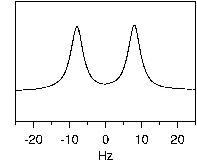
²H spectrum of an aligned protein sample. The sample was 0.5 mM PF0255 aligned in 50 mM Sodium phosphate, 100 mM KCl, 90%H2O and 4% (w/v) C12E5-hexanol bicelles. The ²H splitting measured was 16 Hz, which corresponded to magnitudes of ¹HN-¹⁵N couplings in the range of −9 to 15 Hz.

Examples of spectra

D_HN,N

¹H_N -¹⁵N RDCs can be measured using simple versions of a two-dimensional coupled H-N HSQC. For larger proteins, however, an IPAP version of this sequence (Ottiger et al., 1998) which reduces spectral overlap is preferred. The pulse sequence for this experiment was shown in Figure 2 and examples of this spectrum under isotropic and aligned conditions are shown in Figure 6 for a 13.8 kDa target protein (PF0385). This protein from Pyrococcuss furiosus is annotated only as a conserved hypothetical protein and has no significant sequence identity to anything in the Protein Data Bank. The spectrum is plotted with peaks color coded for the sum and difference of the in-phase and anti-phase components. These are normally observed and analyzed in separate spectral panels. The separation of the two peaks in the vertical dimension is the sum of the RDC and the scalar coupling (D_HN,N + ¹J_HN,N) in the aligned spectrum and the scalar coupling alone in the isotropic spectrum (¹J_HN,N). Note that on alignment the magnitudes of some couplings decrease and the magnitudes of some couplings increase, corresponding to preferred angles near zero and near 90°, respectively. Also note that an increase in the magnitude of a coupling for ¹H_N -¹⁵N actually corresponds to a negative RDC; the scalar one bond coupling is negative for ¹H_N -¹⁵N because of the negative magnetogyric ratio of ¹⁵N. Keeping signs straight is important when multiple types of RDCs are to be combined in a structural analysis.

Figure 6.

IPAP-HSQC of PF0385 under isotropic (Panel A) and aligned (Panel B) conditions. The peaks corresponding to the sum and difference spectra are colored red and black, respectively. ¹⁵N-¹H splittings are indicated. The isotropic sample contained 1 mM PF0385 in 20 mM sodium phosphate, 15 mM KCl, 90% H2O. The aligned sample contained 0.5 mM PF0385 in 20 mM sodium phosphate, 85 mM NaCl, 10 mg/mL Pf1 page, 90% H2O.

A large number of points in the t1 dimension has been collected to provide resolution sufficient for accurate measurement of the coupling (a 100ms acquisition time is usually sufficient). This experiment is generally very sensitive and produces highly accurate coupling values. As an example, data collection for the ¹⁵N coupled HSQC includes 256 complex t1 points, and 2048 t2 points collected over 2 h using a cryogenic probe. Prior to Fourier transformation, data in the direct dimension were corrected for solvent, multiplied by a squared sine bell shifted by 90°, and zero-filled to 4096. Data in the indirect dimension were multiplied by a squared sine bell shifted by 90°, linear predicted from 512 to 1024 and zero-filled to 4096. Peaks were picked using the automated peak picking function in NMRPipe (Delaglio et al, 1995) and inspected manually for accuracy. Peaks were classified as good, slightly overlapped/distorted, and severely overlapped/distorted so that more weight could be given to the most reliable data. Arbitrary peak labels were transferred in automatically from an isotropic HSQC spectrum. J or J+D values were automatically calculated as the difference in Hz between the coupled peaks in the ¹⁵N dimension, and the data were stored in a database for automated recovery and analysis.

D_CαHα, D_Hα(t-1)HN, D_Hα(t)HN

Couplings involving C_α and H_α were collected using a three-dimensional soft HNCA ECOSY (Weisemann et al, 1994). The pulse sequence was shown in Figure 3 and typical spectra are shown in Figure 7 and 8 for a 7.8 kDa target protein (PF0255) under isotropic and aligned conditions. PF0255 is a Pyrococcuss Furiosus protein that was annotated as a DNA-directed RNA polymerase subunit. However it had less than 23% sequence identity to its nearest neighbor in the Protein Data Bank. The HNCA ECOSY experiment provides C_α- H_α couplings in the indirect ¹³C dimension and H_α-H_N couplings in the direct dimension for both intra- and inter-residue peaks. Identification of the inter-residue resonances is aided by the observation that the H_α(i-1) - H_N coupling is zero under isotropic conditions. Examples of this are shown in Figure 7. The pair of peaks at 62 ppm and the pair at 57.5 ppm in the carbon dimension correspond to an inter residue pair and an intra residue pair, respectively. Note that the inter residue pair at 62 ppm in the aligned case shows a small negative splitting. This corresponds to the through space RDC observable for this pair with a four-bond covalent separation. The relative intensity of the peaks can also used be as a guide to assigning intra- and inter-residue status (intra-residue is usually more intense). Even using a sample with a low level of isotopic labeling, the sensitivity of this experiment is adequate for the study of proteins with molecular weight <20 kDa. Despite this being a three-dimensional experiment, there are sometimes issues of spectral overlap that compromise accuracy for the couplings measured. For this reason, we classify the peaks as good, overlapped or questionable, and use larger errors for the less accurate peaks.

Figure 7.

HNCA-E.COSY of PF0255 under isotropic (Panel A) and aligned (Panel B) conditions. ¹Hα-¹HN and ¹Hα(i-1)-¹HN splittings are indicated. The samples contained 1.0 mM PF0255 (isotropic) or 0.5 mM PF0255 (aligned) in 50 mM Sodium phosphate, 100 mM KCl, 90%H2O. The aligned sample contained 4% (w/v) C12E5-hexanol bicelles.

Figure 8.

HNCA-E.COSY strip plot of a fragment of PF0255 connected using Cα chemical shifts and RDCs under isotropic (Panel A) and aligned (Panel B) conditions. The samples contained 1.0 mM PF0255 (isotropic) or 0.5 mM PF0255 (aligned) in 50 mM Sodium phosphate, 100 mM KCl, 90%H2O. The aligned sample contained 4% (w/v) C12E5-hexanol bicelles. Identification of the first residue as a glycine (a triplet owing to the two Hα protons) and the downfield shifting of the Cα of residues 5 and 7 led to the assignment of this fragment to the sequence GKYAIRVR.

The HNCA-ECOSY experiment also provides our primary way of connecting residues that are adjacent in sequence. Since both intra residue and (i)-(i-1) connectivities occur in a single H_N column, an intra residue C_α shift in one column can be matched with an inter-residue C_α shift in another to make the connection. Splittings for a given C_α-H_α pair are also measurable from both sets of cross peaks and the (i)-(i-1) splitting from one column must match the (i) splitting from the second column for the correct connection. Since these splittings vary widely under aligned conditions, this is extremely useful additional connectivity information. The expanded view of the HNCA-E.COSY shown in Figure 8 illustrates the utility of this information.

Fragment connection is performed in a three-step process that is designed to be as efficient and automated as possible. It begins with an automated filter step that eliminates any residue that does not match both peaks in the coupled pair within a given chemical shift cutoff. A generous cutoff of 0.2 ppm in the ¹³C dimension is used to avoid discounting a possible match between weak, overlapped, or distorted peaks. The remaining small number of possible matches is inspected manually using an script written in NMRView (Johnson and Blevins, 1994). This allows classification of possible matches from all spectra, eliminating poor candidates. The final list of possible matches is then run through an algorithm that chains pairs together into possible fragments. All possibilities are saved for later structural analysis when some inconsistent assemblies will be eliminated. The entire process is extremely efficient, taking on the order of 1 hour for a 100 residue protein.

Data collection for the soft HNCA-ECOSY used as an example (0.5mM protein in aligned medium) included 72 t1 (¹³C) points for an acquisition time of about 20 ms, 16 (¹⁵N) t2 points and 2048 t3 points collected over 37 h using a cryogenic probe. Prior to Fourier transformation, data in the direct dimension were apodized as described above and zero-filled to 4096. Data in the ¹³C dimension were linear predicted from 72 to 128, apodized and zero-filled to 256. Data in the ¹⁵N dimension were linear predicted from 16 to 32, apodized and zero-filled to 64. J or J+D values were automatically calculated as the difference in Hz between the coupled peaks in the ¹H and ¹³C dimensions, and stored in a database for automated recovery and analysis. ¹³ C_α chemical shifts were also stored for use in fragment identification (see below).

D_HN-C', D_NC'

Couplings involving the carbonyl carbon are collected using a two-dimensional modified HNCO experiment (Tian et al., 2001) in a manner very similar to that of the coupled HSQC. As seen in the example spectra in Figure 9, the D_NC' and D_HNC' couplings are quite small (1-8 Hz) and are often difficult to measure. Like the HNCA-ECOSY, the multiple ECOSY peaks that appear for each HN lead to overlap. For this reason, an IPAP version (Tian, unpublished results) (Figure 4) was utilized for the larger target protein (PF0385, 13.8 kDa). This experiment may also provide more accurate measurement of the couplings in smaller proteins. The sum and difference spectra (red and black, respectively), have been overlaid to highlight the offsets in both the direct (¹H) and indirect (¹⁵N) dimensions. Note that peaks are displaced along the positive diagonal in the isotropic spectrum indicating that the couplings in the two directions have the opposite sign. But, there are sometimes exceptions in the aligned case. Since the RDC contribution to the CN splitting is never larger than the scalar coupling, we know this coupling to be negative, and the direction of the offset allows determination of the absolute sign of the RDC.

Figure 9.

IPAP-HNCO of PF0385 under isotropic (Panel A) and aligned (Panel B) conditions. The samples were 1 mM PF0385 in 20 mM Sodium phosphate, 15 mM KCl, 90%H2O for isotropic and the same buffer, 85 mM NaCl, 10 mg/mL Pf1 phage for aligned. The peaks corresponding to the sum and difference spectra are colored red and black, respectively.

Data collection for the IPAP-HNCO shown included 256 t1 points, and 2048 t2 points over 16 h. Prior to Fourier transformation, data in the direct dimension were apodized and zero-filled to 4096. Data in the ¹⁵N dimension were linear predicted from 256 to 512, apodized and zero-filled to 4096. The data were processed using IPAP scripts that combined the in-phase and anti-phase signals to give two spectra: the sum and difference. Peaks were picked from both spectra, and the peak lists combined to allow for calculation of the RDCs. J or J+D values were automatically calculated as the difference in Hz between the coupled peaks in the ¹⁵N or ¹H dimension, and the data were stored in a database for automated recovery and analysis.

An ¹⁵N-edited NOESY-HSQC was also collected to aid in fragment assembly of the two proteins discussed. Identification of a small number (typically about a dozen) of inter-fragment NOEs provides information on the spatial arrangement of the fragments. The NOESY-HSQC is typically collected with 128 t1 points, 16 t2 points and 2048 t3 points over 16 h. Also a TOCSY-HSQC was collected in parallel with the NOESYHSQC. This provides a convenient way of correlating H_α resonance position to HSQC cross peaks for use in assignment of NOE constraints. In addition, information about amino acid type can be obtained and utilized for sequence-specific assignment of fragments.

Data Analysis

Data assessment from powder patterns

Before embarking on the task of structure determination it is advantageous to make a general assessment of the quality of various types of data and identify any anomalous points that may contaminate analysis. One simple tool is a direct comparison of distributions RDCs from different nuclear pairs (histograms showing the number of couplings measured at each possible coupling value). In principle, with a sufficiently large number of couplings, all space should be sampled and powder patterns should result that differ only by scaling factors related to the sizes of magnetogyric ratios for the coupled nuclei, the signs of these ratios, and distances between nuclei. Any inexplicable differences between two different sources of data will highlight systematic errors in data treatment (such as incorrect assumptions about signs of couplings); the patterns will also help to identify outliers that need to be manually reexamined, and they will give estimates of order parameters that can be used as useful filters for proper geometric solutions.

The first step in performing a powder pattern analysis is the conversion of all RDC values from units of Hz to unit-less measurements. This conversion can be performed using Eq. 3 below.

$$s=\frac{D\times r^3}{D_{\mathit{Max}}}$$ (3)

Here D denotes the experimental data, r is the length of the inter-nuclear vector that joins the two nuclei of interest and D_max is the maximum observable RDC for two nuclei at 1Å distance under perfect alignment. Values for D_max and r used in our calculations are shown in Table 1. Figure 10 below illustrates a comparison of the distribution of RDCs for ¹H-¹⁵N and ¹H-¹³C_α couplings. Rather than plotting simple histograms, smoothed curves have been plotted utilizing Parsen density estimation (Fukunaga, 1990). The data are for PF0255, the same protein used to illustrate the HNCA-ECOSY data set described above.

Table 1.

Maximum RDC values and bond distances.

	Dmax	r (Å)
C-N	6125	1.335
N-HN	24350	1.010
C-H	−60400	2.035
Cα-Hα	−60400	1.090

Figure 10.

Distributions of N-H_N and C_α-H_α RDCs

The agreement shown in Figure 10 is fairly good. There is a possible outlier at a value of –0.0007 in the C_α-H_α set. This data point was checked and appeared to be a valid measurement. Outlying data may not in all cases be due to error but may be due to sparse sampling of vectors in space. Also, in the case of C_α-H_α data, the outliers can originate from Glycines since the coupling value is often reported as the sum of both C_α-Hα1 and C_α-H_α2 residual dipolar couplings.

The fact that the central maximum lies at a negative value for both distributions in Figure 10 suggests that the relative signs of couplings have been assigned properly (largest couplings negative for C_α-H_α and positive for H-N). A simplistic analysis of the shape of the distribution would assign extreme values to S_zz and S_yy in accord with the convention S_zz|≥| S_yy . The third order parameter (S_xx) can be calculated by utilizing the traceless property of the order tensor (S_xx=-S_zz-S_yy). Data for H-N measurements in Figure 10 would set S_zz = 0.00075, S_yy = -0.0006, and S_xx = -0.00015. It can theoretically be proven that the most frequently observed value of RDC for a uniformly-distributed set of vectors in space is the value corresponding to S_xx (Valafar and Prestegard, 2003; Varner et al., 1996). This would imply that the highest peak in the powder pattern should correspond to S_xx. This is again consistent with the numbers suggested above. Other more sophisticated methods such as maximum likelihood (Warren and Moore, 2001) can be employed to provide a better estimate of the order parameters by fitting the entire powder pattern rather than just the extrema.

The above order parameter estimates can be used as additional filters for fragment geometry solutions coming from the program to be described in the next section. The number of data points used to find allowed geometries and order matrix elements will be small and false geometries can easily arise in combination with principal order parameters that are inconsistent with the distributions described above. Once several fragments with reliable geometries and consistent order parameters are found, it is often better to substitute principal order parameters from fragment solutions for the powder pattern estimates described above.

Structure Determination using REDCRAFT

The actual search for fragment geometries consistent with RDC data is performed by a program named REDCRAFT (REsidual Dipolar Coupling based Residue Assembly and Filtering Tool) (H. Valafar, manuscript in preparation). This program runs as either a single processor version or a Linux cluster version. As described in the introduction, it constructs backbone geometries for peptide fragments in a manner consistent with allowed Ramachandran space, measured ³J_HN-Hα scalar couplings, and an experimentally collected set of RDCs.

Although the program itself is very general, the input for the current version has been tailored to the particular set of couplings produced by the experiments described above. This input consists of repeating blocks of data in the format described in Table 2, one block for every residue of the fragment. The first line of a block begins with designation of the amino acid type for the residue. Because we work only with backbone data, and side chains are irrelevant, types are designated as either GLY (signifying Glycine) or ALA (signifying Alanine). The line continues with ³J_HN-Hα for the residue and concludes with a comment. Comments can be any string data, but we find this field a convenient place to store residue numbers or peak numbers that correlate data with peaks in a reference ¹⁵N-¹H HSQC data set.

Table 2.

Repeating blocks of data for REDCRAFT input (format left, example right).

AA type	3JHN-Hα	Comments	GLY	15.792	Peak 52
DC-N	ε C-N		1.745	2
DN-HN	ε N-HN		3.715	1
DC-H	ε C-H		−8.034	1.333
DCα-Hα	ε Cα-Hα		−30.35	1	Sum of Ds
DHα-HN	ε Hα-HN		5.985	0.888	Sum of Ds
DHα(i-1)-HN	ε Hα(i-1)-HN		−1.075	1.333
AA type	3JHN-Hα	Comments	ALA	4.2581	Peak 20
DC-N	ε C-N		0.316	1.333
DN-HN	ε N-HN		−9.039	1
DC-H	ε C-H		−0.209	0.888	weak
DCα-Hα	ε Cα-Hα		−14.938	1
DHα-HN	ε Hα-HN		2.528	1.333
DHα(i-1)-HN	ε Hα(i-1)-HN		−0.68	1.333	Sum of Ds

The remaining six lines begin with one of the six RDCs that can be detected through a particular ¹⁵N-¹H_N pair (in Hz with the proper sign). Note that in the case of Glycines, the D_Cα-Hα is actually D_Cα1-Hα1+ D_Cα2-Hα2. Similarly, the value of the ³J_HN-Hα is reported as the sum of both couplings, and for a residue following Glycine, the D_Hα(i-1)-HN value is reported as a sum value. Any missing RDCs are indicated as 999. Each coupling is followed by a scaling factor that is used to account for the information content of the various couplings, and concludes with another comment field. The scaling factors are based on the ratio of the maximum coupling for a given entry relative to D_max,N-HN (Table 1) and the reciprocal of the ratio of estimated percentage experimental error for a given entry relative to a standard error for D_HN-N. The result is a simple ratio of the estimated average error of HN couplings relative to error of the coupling in question. Because of structural noise, errors for our more precise measurements are often set to 10% of the range of couplings observed. Others reflect experimental precision of measurement with reasons for deviation often included in the comment field. REDCRAFT can take multiple input files, with each one containing data from a different orientation medium. In this case a common geometry satisfying all data is found.

The time required for geometry searches depends on the depth of search into the ranked lists of allowed ϕ and ψ angles for each dipeptide fragment to be joined. Fragments as large as 20 residues can be processed using the parallel version of REDCRAFT with a reasonable search depth (1000) in less than a few hours. An entire protein of size 70 residues can be processed in less than a day. Under the conditions where data are numerous and of sufficiently high quality (such as Rubredoxin; BMRB accession #5926), the search depth can be quite shallow and a 25 residue fragment can be successfully processed under an hour on a typical desktop computer.

The final outcome of this analysis consists of a single file containing a ranked list of all examined structures. These are described by departures in ϕ and ψ from the extended starting conformation (IUPAC angles can be obtained by subtracting 180°). The top entry will be the geometry that best fits the experimental RDCs. Table 3 shows every tenth entry for the top 100 solutions produced by REDCRAFT for a 7 residue fragment from the C-terminus of the PF0255 protein (K46-V52). The last column indicates the rmsd between the back calculated scaled RDCs (using the best solution order tensor for the given geometry) and the measured RDCs. The data used in this particular calculation included 38 RDCs from alignment in a bacteriophage medium and 24 RDCs from alignment in a C12E5/hexanol bicelle medium. The derived conformation obviously agrees well with the data as indicated by the rmsd values and clustering of the ϕ and ψ values. The particular segment examined terminates because of a proline in the next position. A second segment can be examined independently beginning with the residue after proline (G54-R61).

Table 3.

Sampling of top 100 solutions for a fragment of 7 residues (results in 6 sets of torsion angles being determined).

Δφ1	Δψ1	Δφ2	Δψ2	Δφ3	Δψ3	Δφ4	Δψ4	Δφ5	Δψ5	Δφ6	Δψ6	RMSD
−70	−40	−80	−60	−90	170	90	30	−70	100	−90	150	1.843248
−70	−40	−80	−50	−90	170	90	30	−70	100	−90	150	1.888763
−70	−40	−70	−60	−90	170	90	30	−70	100	−90	140	1.914637
−70	−30	−80	−50	−90	170	90	30	−70	100	−90	150	1.92957
−70	−40	−70	−60	−90	170	100	30	−70	100	−100	150	1.93773
−70	−30	−80	−60	−90	170	100	40	−80	100	−100	150	1.94264
−80	−30	−80	−60	−80	170	90	40	−80	100	−90	150	1.949104
−70	−30	−80	−60	−90	170	100	30	−80	100	−90	150	1.955443
−70	−30	−80	−60	−80	170	90	30	−70	100	−90	160	1.959502
−70	−40	−70	−60	−80	170	90	30	−70	100	−90	150	1.965129

In the case presented we were able to sequentially place the fragments as being before and after proline 53. REDCRAFT is able to accommodate missing data, including that for an entire residue such as proline. Therefore, an entire 16 residue segment was also assembled using 67 RDCs for the first medium and 57 RDCs from the second medium. As a final option in the REDCRAFT determination protocol angles determined for each fragment can be locally refined to obtain a better match with the RDCs. This is done by a simple implementation of Monte Carlo sampling of a window size indicated by the user (usually +/− 5° for a 10° grid size).. At the end of this procedure, a perl script (Mol_Scr.prl) is used to generate a script for MolMol (Koradi et al., 1996) to construct the atomic coordinates of the fragments. The predicted structure coming from this procedure applied to the entire 16 residue C-terminal fragment of PF0255 will be described more completely below.

Fragment validation using REDCAT

Upon the successful determination of fragment geometries, it is important to perform a more detailed error analysis. This can be done with the program REDCAT (REsidual Dipolar Coupling Analysis Tool) (Valafar and Prestegard, 2004). The atomic coordinates produced from the previous section, along with the RDCs used to determine the coordinates, can serve as input for the program. Using the “Prepare Input File” and “Import RDC” functions of this program, one can conveniently produce REDCAT input files. The first step for confirmation of a structure is to perform an error analysis and inspect the individual contributions of each piece of RDC data to the overall RMSD reported by REDCRAFT. Large contributions should originate only from entries that have been identified as inaccurate measurements. Other large errors can result if there are segments with substantial degrees of internal motion (spin relaxation measurements or amide proton exchange experiments can be used to independently identify these segments) or from simple mis-assignments. In either case this may be cause for a re-determination of fragment geometry with the problematic data corrected or eliminated. REDCAT also provides solutions for principal order parameters. In cases of multiple fragments it is important to verify that these are consistent between fragments, usually within 15% for S_zz and 30% for S_xx and S_yy.

Fragment orientation using REDCAT

In cases where multiple fragments, as opposed to one continuous fragment, are obtained from REDCRAFT, it is important to put each fragment in its principal alignment frame (PAF) for assembly into a complete molecule. Once each fragment has been described in its PAF, RDCs from a second alignment medium can be used to resolve inversion degeneracies (Al-Hashimi et al., 2000; Mayer, 2004), and then fragments can be translated under NOE and covalent constraints to produce a final structure. REDCAT offers tools to solve for the angles that transform a fragment to its principal alignment frame and to rotate initial fragment coordinates into that principal alignment frame. This rotation is an important step in assembling an intact structure when connectivities between residues terminate periodically throughout the length of the protein sequence. Even without direct connection the proper relative orientations of separate fragments can be determined because fragments from the same structure must share a common alignment frame. The frame produced by REDCAT is actually arbitrarily chosen from a four-fold degenerate set that differs by rotations of 180º about each of the three Cartesian axes. In assembling fragments the degeneracy can be resolved by comparing the possible relative orientations of two fragments as determined in two different alignment media. In general, relative orientations will appear the same for only one choice within the degenerate sets. The process is illustrated in Figure 11 for the pre- and post-proline pieces in the C-terminal segment of PF0255. In this illustration the pieces have been produced by dividing the sixteen-residue structure produced by REDCAT at the proline, but the process would be the same had the proper sequential connection through proline not been found. At the left of each line in the figure is the first half of the segment. This is followed by the second half in each of the four degenerate PAF frames. The first line is from a sample aligned in bacteriophage. The second line is from a sample aligned in C5E12/hexanol bicelles. All structures in the second line have been rotated by transformations that superimpose the first half fragment of the second line with the first half fragment in the first line. Note that only relative orientations involving the 53-58ref structure in line one and the 53-58y structure in line two appear the same. This points to the proper relative orientation for assembly. It is also reassuring that this puts the C-terminus of the first half in proximity to the N-terminus of the second half for easy covalent connection through a proline.

Figure 11.

Fragment alignment using RDC data for PF0255 from two different media. At the left of each line is the piece of the fragment before proline 53. The remaining four depictions of the piece after proline have been produced by rotating the reference structure by 180° about x, y, and z axes of the principal alignment frame. The structures in the second line have been rotated to overlay the first piece in both lines using the program chimera(Huang, 1996).

In general, when fragment geometries and alignments have been determined separately as described above, we will not have placed these connected sets of residues into a position in the overall sequence prior to fragment structure determination. In cases where we have to rely primarily on data from the three RDC experiments described above we can use a program named SEASCAPE (Sequential Assignment by Structure and Chemical shift Aided Probablity Estimation) to aid in this placement. This program relies on the information content of C_α chemical shifts of connected sets of residues once the secondary structure (ϕ,ψ) dependence is removed (Morris et al., 2004). Essentially the connected fragment, with its associated ϕ,ψ angles and C_α shift, is moved along the sequence calculating a probability score for each placement. This is depicted in Figure 12 for the two halves of the C-terminal fragment of PF0255. Fragment 1 (minus the first residue) has only one position in the sequence where the probability score is significant (height of bar), namely beginning at residue 47. Fragment 2 (using only data for 54-58) has two positions with significant probability for placement, but the most probable begins at residue 54. It is clear that the two fragments could have been correctly placed on either side of the central proline based on just C_α shifts and local structure information.

Figure 12.

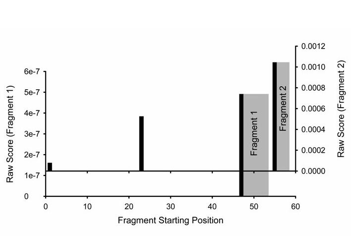
Sequential placement of fragments using local structure and C_α chemical shifts. Fragment 1, based on highest probability, is positioned beginning with K47 and ending with V52. The position of the first residue in the fragment is indicated with a black bar while placement of the subsequent residues is shown in gray. No other placement has significant probability. Placement of fragment 2, again based on hightest probability, begins with G54 and ends with A57. While other positions are possible, beginning with G1 or G23, the relative probabilities are half or less than that of beginning position G54.

Translation to connect fragments in the example shown here will be done only under constraints from the allowed geometry of the connecting proline. In general small numbers of backbone-to-backbone NOE constraints would be added. For a trans proline the appropriate distance between CO in the first half and N of the residue following proline in the second half is 3.2-4.2 Å. The terminal phi and psi angles of each fragment are not well defined and free rotation of these is allowed in making connections. This final structure can be refined with programs such as XPLOR-NIH (Schwieters et al., 2003) to add missing residues, optimize bond geometry, and translate fragments.

Structure quality assesment

For the C-terminus of PF0255 used in the illustrations above there is now an X-ray structure (PDB # 1RYQ) that allows evaluation of the final structure produced by REDCRAFT. This structure was determined by the X-ray component of our pilot center during the course of our investigations (B.C. Wang et al, manuscript in preparation). We will discuss only the NMR results from the fragment produced by running the intact 16 residue segment discussed above. A least squares overlay of the backbone atoms from the central part of the segment (residues 45-57) produces an rmsd from the X-ray structure of 1.1 Å. This overlay is depicted in Figure 13. The entire X-ray structure is shown for illustration. Additional fragments were in fact determined by the NMR approach, but agreement diverges at the amino terminus. This is largely because the NMR structure was pursued on an apo form of this Zn/Fe protein, and without metal the amino terminus is partially disordered. However, the excellent agreement for the C-terminal segment demonstrates the feasibility of constructing accurate backbone structures using primarily RDC information.

Figure 13.

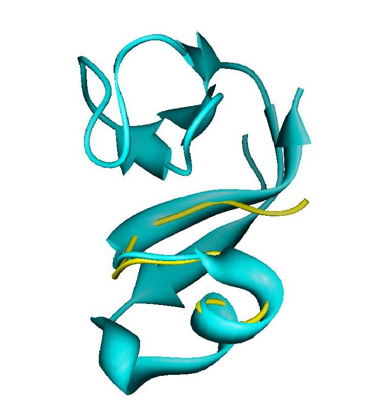
Backbone superimposition of the RDC based structure for residues 46-58 of PF0255 on the corresponding segment from the X-ray structure: 1RYQ.

In order to meet efficiency objectives of the structural genomics initiative, the procedure we have outlined was designed to use a small subset of RDC data acquisition experiments, and to proceed independently of separate resonance assignment experiments. For other applications, there will certainly be other useful experiments for the measurement of RDCs, and there may be sound reasons to conduct experiments directed at independent sequential assignments. However, the data analysis tools we have described are quite generally applicable and should be useful in analyzing these expanded sets of data. For the future, application to larger proteins is clearly an important goal. Although we expect applications to proteins of 20 kDa to be possible with the procedure described, applications have so far been only to proteins under 15 kDa. Moving beyond this limit will certainly require alteration in the types of experiment used to acquire RDCs, the use of more extensive experiments for independent assignment, and the incorporation of more complementary data, such as that from NOEs, or relaxation enhancement by paramagnetic sites.

References

- Adams MWW, Dailey HA, Delucas LJ, Luo M, Prestegard JH, Rose JP, Wang BC. The Southeast Collaboratory for Structural Genomics: A high-throughput gene to structure factory. Accounts of Chemical Research. 2003;36:191–198. doi: 10.1021/ar0101382. [DOI] [PubMed] [Google Scholar]
- Alexandrescu AT, Kammerer RA. Structure and disorder in the ribonuclease S-peptide probed by NMR residual dipolar couplings. Protein Science. 2003;12:2132–2140. doi: 10.1110/ps.03164403. [DOI] [PMC free article] [PubMed] [Google Scholar]
- Al-Hashimi HM, Patel DJ. Residual dipolar couplings: Synergy between NMR and structural genomics. Journal of Biomolecular Nmr. 2002;22:1–8. doi: 10.1023/a:1013801714041. [DOI] [PubMed] [Google Scholar]
- Al-Hashimi HM, Valafar H, Terrell M, Zartler ER, Eidsness MK, Prestegard JH. Variation of molecular alignment as a means of resolving orientational ambiguities in protein structures from dipolar couplings. Journal of Magnetic Resonance. 2000;143:402–406. doi: 10.1006/jmre.2000.2049. [DOI] [PubMed] [Google Scholar]
- Andrec M, Du P, Levy RM. Protein backbone structure determination using only residual dipolar couplings from one ordering medium. J Biomol NMR. 2001a;21:335–347. doi: 10.1023/a:1013334513610. [DOI] [PubMed] [Google Scholar]
- Andrec M, Du P, Levy RM. Protein structural motif recognition via NMR residual dipolar couplings. J Am Chem Soc. 2001b;123:1222–1229. doi: 10.1021/ja003979x. [DOI] [PubMed] [Google Scholar]
- Assfalg M, Bertini I, Turano P, Mauk AG, Winkler JR, Gray HB. N-15-H-1 residual dipolar coupling analysis of native and alkaline-K79A Saccharomyces cerevisiae cytochrome c. Biophysical Journal. 2003;84:3917–3923. doi: 10.1016/S0006-3495(03)75119-4. [DOI] [PMC free article] [PubMed] [Google Scholar]
- Barbieri R, Bertini I, Cavallaro G, Lee YM, Luchinat C, Rosato A. Paramagnetically induced residual dipolar couplings for solution structure determination of lanthanide binding proteins. Journal of the American Chemical Society. 2002;124:5581–5587. doi: 10.1021/ja025528d. [DOI] [PubMed] [Google Scholar]
- Bax A, Kontaxis G, Tjandra N. Dipolar couplings in macromolecular structure determination. Methods Enzymol. 2001;339:127–174. doi: 10.1016/s0076-6879(01)39313-8. [DOI] [PubMed] [Google Scholar]
- Beraud S, Bersch B, Brutscher B, Gans P, Barras F, Blackledge M. Direct structure determination using residual dipolar couplings: Reaction-site conformation of methionine sulfoxide reductase in solution. Journal of the American Chemical Society. 2002;124:13709–13715. doi: 10.1021/ja0268783. [DOI] [PubMed] [Google Scholar]
- Burley SK, Almo SC, Bonanno JB, Capel M, Chance MR, Gaasterland T, Lin DW, Sali A, Studier FW, Swaminathan S. Structural genomics: beyond the Human Genome Project. Nature Genetics. 1999;23:151–157. doi: 10.1038/13783. [DOI] [PubMed] [Google Scholar]
- Chance MR, Bresnick AR, Burley SK, Jiang JS, Lima CD, Sali A, Almo SC, Bonanno JB, Buglino JA, Boulton S, et al. Structural genomics: A pipeline for providing structures for the biologist. Protein Science. 2002;11:723–738. doi: 10.1110/ps.4570102. [DOI] [PMC free article] [PubMed] [Google Scholar]
- Clore GM, Schwieters CD. Docking of protein-protein complexes on the basis of highly ambiguous intermolecular distance restraints derived from 1H/15N chemical shift mapping and backbone 15N-1H residual dipolar couplings using conjoined rigid body/torsion angle dynamics. J Am Chem Soc. 2003;125:2902–2912. doi: 10.1021/ja028893d. [DOI] [PubMed] [Google Scholar]
- Cornilescu G, Delaglio F, Bax A. Protein backbone angle restraints from searching a database for chemical shift and sequence homology. Journal of Biomolecular Nmr. 1999;13:289–302. doi: 10.1023/a:1008392405740. [DOI] [PubMed] [Google Scholar]
- de Alba E, Tjandra N. NMR dipolar couplings for the structure determination of biopolymers in solution. Progress in Nuclear Magnetic Resonance Spectroscopy. 2002;40:175–197. [Google Scholar]
- Delaglio F, Grzesiek S, Vuister GW, Zhu G, Pfeifer J, Bax A. Nmrpipe - a Multidimensional Spectral Processing System Based on Unix Pipes. Journal of Biomolecular Nmr. 1995;6:277–293. doi: 10.1007/BF00197809. [DOI] [PubMed] [Google Scholar]
- Delaglio F, Kontaxis G, Bax A. Protein Structure Determination Using Molecular Fragment Replacement and NMR Dipolar Couplings. Journbal of the American Chemical Soceity. 2000;122:2142–2143. [Google Scholar]
- Dosset P, Hus JC, Marion D, Blackledge M. A novel interactive tool for rigid-body modeling of multi-domain macromolecules using residual dipolar couplings. Journal of Biomolecular Nmr. 2001;20:223–231. doi: 10.1023/a:1011206132740. [DOI] [PubMed] [Google Scholar]
- Fesik SW. NMR as a tool in drug research. Faseb Journal. 1999;13:A1422–A1422. [Google Scholar]
- Fesik SW. The use of NMR in cancer drug discovery. Clinical Cancer Research. 2001;7:3827s–3827s. [Google Scholar]
- Fukunaga K. Introduction to Statistical Pattern Recognition. 2nd edn. Academic Press; 1990. Incorporated. [Google Scholar]
- Hajduk PJ, Betz SF, Mack J, Ruan XA, Towne DL, Lerner CG, Beutel BA, Fesik SW. A strategy for high-throughput assay development using leads derived from nuclear magnetic resonance-based screening. Journal of Biomolecular Screening. 2002;7:429–432. doi: 10.1177/108705702237674. [DOI] [PubMed] [Google Scholar]
- Hajduk PJ, Meadows RP, Fesik SW. NMR-based screening in drug discovery. Quarterly Reviews of Biophysics. 1999;32:211–240. doi: 10.1017/s0033583500003528. [DOI] [PubMed] [Google Scholar]
- Haliloglu T, Kolinski A, Skolnick J. Use of residual dipolar couplings as restraints in ab initio protein structure prediction. Biopolymers. 2003;70:548–562. doi: 10.1002/bip.10511. [DOI] [PubMed] [Google Scholar]
- Hansen MR, Mueller L, Pardi A. Tunable alignment of macromolecules by filamentous phage yields dipolar coupling interactions. Nature Structural Biology. 1998;5:1065–1074. doi: 10.1038/4176. [DOI] [PubMed] [Google Scholar]
- Huang CC, Couch GS, et al. Chimera: An Extensible Molecular Modeling Application Constructed Using Standard Components; Paper presented at: Pacific Symposium on Biocomputing.1996. [Google Scholar]
- Hus JC, Marion D, Blackledge M. De novo determination of protein structure by NMR using orientational and long-range order restraints. Journal of Molecular Biology. 2000;298:927–936. doi: 10.1006/jmbi.2000.3714. [DOI] [PubMed] [Google Scholar]
- Johnson BA, Blevins RA. Nmr View - a Computer-Program for the Visualization and Analysis of Nmr Data. Journal of Biomolecular Nmr. 1994;4:603–614. doi: 10.1007/BF00404272. [DOI] [PubMed] [Google Scholar]
- Koradi R, Billeter M, Wuthrich K. MOLMOL: A program for display and analysis of macromolecular structures. Journal of Molecular Graphics. 1996;14:51. doi: 10.1016/0263-7855(96)00009-4. [DOI] [PubMed] [Google Scholar]
- Lin YJ, Dancea F, Lohr F, Klimmek O, Pfeiffer-Marek S, Nilges M, Wienk H, Kroger A, Ruterjans H. Solution structure of the 30 kDa polysulfide-sulfur transferase homodimer from Wolinella succinogenes. Biochemistry. 2004;43:1418–1424. doi: 10.1021/bi0356597. [DOI] [PubMed] [Google Scholar]
- Losonczi JA, Andrec M, Fischer MWF, Prestegard JH. Order matrix analysis of residual dipolar couplings using singular value decomposition. Journal of Magnetic Resonance. 1999;138:334–342. doi: 10.1006/jmre.1999.1754. [DOI] [PubMed] [Google Scholar]
- MacArthur MW, Thornton JM. Deviations from planarity of the peptide bond in peptides and proteins. Journal of Molecular Biology. 1996;264:1180–1195. doi: 10.1006/jmbi.1996.0705. [DOI] [PubMed] [Google Scholar]
- Mayer BJ, Valafar H, Leblond P, Prestegard JH. Backbone Structure of a Conserved Hypothetical Protein using Residual Dipolar Couplings. J Struct Funct Genomics. 2004 doi: 10.1007/s10969-005-4899-5. submitted. [DOI] [PMC free article] [PubMed] [Google Scholar]
- Montelione GT, Zheng DY, Huang YPJ, Gunsalus KC, Szyperski T. Protein NMR spectroscopy in structural genomics. Nature Structural Biology. 2000;7:982–985. doi: 10.1038/80768. [DOI] [PubMed] [Google Scholar]
- Morris LC, Valafar H, Prestegard JH. Assignment of protein backbone resonances using connectivity, torsion angles and C-13(alpha) chemical shifts. Journal of Biomolecular Nmr. 2004;29:1–9. doi: 10.1023/B:JNMR.0000019500.76436.31. [DOI] [PubMed] [Google Scholar]
- Nair M, McIntosh PB, Frenkiel TA, Kelly G, Taylor IA, Smerdon SJ, Lane AN. NMR structure of the DNA-binding domain of the cell cycle protein Mbp1 from Saccharomyces cerevisiae. Biochemistry. 2003;42:1266–1273. doi: 10.1021/bi0205247. [DOI] [PubMed] [Google Scholar]
- Norvell JC, Machalek AZ. Structural genomics programs at the US National Institute of General Medical Sciences - Foreword. Nature Structural Biology. 2000;7:931–931. doi: 10.1038/80694. [DOI] [PubMed] [Google Scholar]
- Ohnishi S, Lee AL, Edgell MH, Shortle D. Direct demonstration of structural similarity between native and denatured eglin C. Biochemistry. 2004;43:4064–4070. doi: 10.1021/bi049879b. [DOI] [PubMed] [Google Scholar]
- Ottiger M, Delaglio F, Bax A. Measurement of J and dipolar couplings from simplified two-dimensional NMR spectra. J Magn Reson. 1998;131:373–378. doi: 10.1006/jmre.1998.1361. [DOI] [PubMed] [Google Scholar]
- Prestegard JH, Al-Hashimi HM, Tolman JR. NMR structures of biomolecules using field oriented media and residual dipolar couplings. Quarterly Reviews of Biophysics. 2000;33:371–424. doi: 10.1017/s0033583500003656. [DOI] [PubMed] [Google Scholar]
- Prestegard JH, Bougault CM, Kishore AI. Residual dipolar coupling in structure detrmination of biomolecules. Chemical Reviews. 2004;104 doi: 10.1021/cr030419i. 0000-0000. [DOI] [PubMed] [Google Scholar]
- Prestegard JH, Kishore AI. Partial alignment of biomolecules: an aid to NMR characterization. Current Opinion in Chemical Biology. 2001;5:584–590. doi: 10.1016/s1367-5931(00)00247-7. [DOI] [PubMed] [Google Scholar]
- Rohl CA, Baker D. De novo determination of protein backbone structure from residual dipolar couplings using rosetta. Journal of the American Chemical Society. 2002;124:2723–2729. doi: 10.1021/ja016880e. [DOI] [PubMed] [Google Scholar]
- Ruckert M, Otting G. Alignment of biological macromolecules in novel nonionic liquid crystalline media for NMR experiments. Journal of the American Chemical Society. 2000;122:7793–7797. [Google Scholar]
- Saupe A. Recent results in the field of liquid crystals. Angew Chem, Int Ed Engl. 1968;7:97. [Google Scholar]
- Schwieters CD, Kuszewski JJ, Tjandra N, Clore GM. The Xplor-NIH NMR molecular structure determination package. Journal of Magnetic Resonance. 2003;160:65–73. doi: 10.1016/s1090-7807(02)00014-9. [DOI] [PubMed] [Google Scholar]
- Sklenar V, Piotto M, Leppik R, Saudek V. Gradient-Tailored Water Suppression for H-1-N-15 Hsqc Experiments Optimized to Retain Full Sensitivity. Journal of Magnetic Resonance Series A. 1993;102:241–245. [Google Scholar]
- Tian F, Valafar H, Prestegard JH. A dipolar coupling based strategy for simultaneous resonance assignment and structure determination of protein backbones. Journal of the American Chemical Society. 2001;123:11791–11796. doi: 10.1021/ja011806h. [DOI] [PubMed] [Google Scholar]
- Tolman JR. Dipolar couplings as a probe of molecular dynamics and structure in solution. Curr Opin Struct Biol. 2001;11:532–539. doi: 10.1016/s0959-440x(00)00245-1. [DOI] [PubMed] [Google Scholar]
- Tossavainen H, Permi P, Annila A, Kilpelainen I, Drakenberg T. NMR solution structure of calerythrin, an EF-hand calcium-binding protein from Saccharopolyspora erythraea. European Journal of Biochemistry. 2003;270:2505–2512. doi: 10.1046/j.1432-1033.2003.03623.x. [DOI] [PubMed] [Google Scholar]
- Valafar H, Prestegard JH. Rapid classification to a protein fold family using a statistical analysis of dipolar couplings. Bioinformatics. 2003;19:1–8. doi: 10.1093/bioinformatics/btg201. [DOI] [PubMed] [Google Scholar]
- Valafar H, Prestegard JH. REDCAT: a residual dipolar coupling analysis tool. J Magn Reson. 2004;167:228–241. doi: 10.1016/j.jmr.2003.12.012. [DOI] [PubMed] [Google Scholar]
- Varner SJ, Vold RL, Hoatson GL. An efficient method for calculating powder patterns. Journal of Magnetic Resonance Series A. 1996;123:72–80. doi: 10.1006/jmra.1996.0215. [DOI] [PubMed] [Google Scholar]
- Wang YX, Marquardt JL, Wingfield P, Stahl SJ, Lee-Huang S, Torchia D, Bax A. Simultaneous measurement of H-1-N-15, H-1-C-13 ', and N-15-C-13 ' dipolar couplings in a perdeuterated 30 kDa protein dissolved in a dilute liquid crystailine phase. Journal of the American Chemical Society. 1998;120:7385–7386. [Google Scholar]
- Warren JJ, Moore PB. A maximum likelihood method for determining D-a(PQ) and R for sets of dipolar coupling data. Journal of Magnetic Resonance. 2001;149:271–275. doi: 10.1006/jmre.2001.2307. [DOI] [PubMed] [Google Scholar]
- Weaver JL, Prestegard JH. Nuclear magnetic resonance structural and ligand binding studies of BLBC, a two-domain fragment of barley lectin. Biochemistry. 1998;37:116–128. doi: 10.1021/bi971619p. [DOI] [PubMed] [Google Scholar]
- Weisemann R, Ruterjans H, Schwalbe H, Schleucher J, Bermel W, Griesinger C. Determination of H(N),H-Alpha and H(N), C' Coupling-Constants in C-13,N-15-Labeled Proteins. Journal of Biomolecular Nmr. 1994;4:231–240. doi: 10.1007/BF00175250. [DOI] [PubMed] [Google Scholar]
- Wishart DS, Sykes BD. The C-13 Chemical-Shift Index - a Simple Method for the Identification of Protein Secondary Structure Using C-13 Chemical-Shift Data. Journal of Biomolecular Nmr. 1994;4:171–180. doi: 10.1007/BF00175245. [DOI] [PubMed] [Google Scholar]
- Wishart DS, Sykes BD, Richards FM. The Chemical-Shift Index - a Fast and Simple Method for the Assignment of Protein Secondary Structure through Nmr-Spectroscopy. Biochemistry. 1992;31:1647–1651. doi: 10.1021/bi00121a010. [DOI] [PubMed] [Google Scholar]
- Wohnert J, Franz KJ, Nitz M, Imperiali B, Schwalbe H. Protein alignment by a coexpressed lanthanide-binding tag for the measurement of residual dipolar couplings. J Am Chem Soc. 2003;125:13338–13339. doi: 10.1021/ja036022d. [DOI] [PubMed] [Google Scholar]
- Wood MJ, Komives EA. Production of large quantities of isotopically labeled protein in Pichia pastoris by fermentation. Journal of Biomolecular Nmr. 1999;13:149–159. doi: 10.1023/a:1008398313350. [DOI] [PubMed] [Google Scholar]
- Zheng DY, Aramini JM, Montelione GT. Validation of helical tilt angles in the solution NMR structure of the Z domain of Staphylococcal protein A by combined analysis of residual dipolar coupling and NOE data. Protein Science. 2004;13:549–554. doi: 10.1110/ps.03351704. [DOI] [PMC free article] [PubMed] [Google Scholar]
- Zhou HJ, Vermeulen A, Jucker FM, Pardi A. Incorporating residual dipolar couplings into the NMR solution structure determination of nucleic acids. Biopolymers. 1999;52:168–180. doi: 10.1002/1097-0282(1999)52:4<168::AID-BIP1002>3.0.CO;2-7. [DOI] [PubMed] [Google Scholar]