A Parallel Tracking Method for Acoustic Radiation Force Impulse Imaging

Abstract

Radiation force-based techniques have been developed by several groups for imaging the mechanical properties of tissue. Acoustic Radiation Force Impulse (ARFI) imaging is one such method that uses commercially available scanners to generate localized radiation forces in tissue. The response of the tissue to the radiation force is determined using conventional B-mode imaging pulses to track micron-scale displacements in tissue. Current research in ARFI imaging is focused on producing real-time images of tissue displacements and related mechanical properties. Obstacles to producing a real-time ARFI imaging modality include data acquisition, processing power, data transfer rates, heating of the transducer, and patient safety concerns. We propose a parallel receive beamforming technique to reduce transducer heating and patient acoustic exposure, and to facilitate data acquisition for real-time ARFI imaging. Custom beam sequencing was used with a Siemens SONOLINE Antares^TM scanner to track tissue displacements with parallel-receive beam-forming in tissue-mimicking phantoms. Using simulations, the effects of material properties on parallel tracking are observed. Transducer and tissue heating for parallel tracking are compared to standard ARFI beam sequencing. The effects of tracking beam position and size of the tracked region are also discussed in relation to the size and temporal response of the region of applied force, and the impact on ARFI image contrast and signal-to-noise ratio are quantified.

I. INTRODUCTION

Radiation force-based imaging is a growing field for imaging the mechanical properties of tissue. Some [1], kinetic acoustic vitreoretinal examination [2], vibro-acoustography [3], and supersonic shear imaging [4].

Acoustic Radiation Force Impulse (ARFI) imaging [5] is a radiation force-based imaging method that uses commercially available ultrasound scanners to generate short duration (approx. 30–300 μs) acoustic radiation forces. These impulses, or pushing pulses, generate localized displacements in tissue of approximately 1–10 μm. The response of the tissue to the radiation force is observed using conventional B-mode imaging pulses to track tissue displacements. Two- or three-dimensional images of tissue displacement can be created by repeating this process along multiple image lines. ARFI imaging is useful for observing lesions that are difficult to visualize with conventional sonography when the lesions are stiffer or softer than the surrounding tissue [5, 6]. ARFI imaging is capable of determining the size and boundaries of these lesions with good contrast [7].

A real-time ARFI imaging system would be a valuable tool for diagnostic purposes as well as for guiding surgical procedures. Real-time ARFI imaging, however, encounters difficulties in data acquisition, processing power, data transfer rates, and low frame rates, and encounters significant challenges with heating of the tissue and transducer [8]. These issues are dependent on the observation time along a line of sight, the number of push locations, and the computational processes.

Although the thermal increases from a single ARFI push are typically less than 0:1°C and can be considered negligible in both the tissue and the transducer, the cumulative effects of real-time, two-dimensional imaging with ARFI can have a significant impact on heating. Palmeri et al. [8] used finite element models to show that temperature increases in tissue can reach up to 4:5°C with an ARFI frame rate of just 3 frames per second (fps), 50 push locations, and an acoustic absorption of 0.5 dB/cm/MHz. Transducer heating is also of concern in real-time ARFI imaging because it can burn the patient and damage the transducer if gone unchecked. The IEC [9] and FDA [10] limit for increase in transducer temperature is 6°C.

Parallel-receive beamforming is a common technique used in B-mode imaging to increase frame rate at little cost to resolution [11]. In supersonic shear imaging, Bercoff et al. [4] uses a parallel beamforming system to monitor shear wave propagation at extremely high frame rates. We propose to adapt parallel beamforming techniques to ARFI imaging in order to concurrently track displacements over multiple, laterally-separated, beam locations for a given pushing pulse. This method can be used to either decrease the heat generated in the transducer and patient while maintaining current frame rates, or to increase the frame rate without further increasing the heat. Our goal is to determine the limits and characteristics of a parallel tracking system for real-time ARFI imaging that will be diagnostically useful.

II. BACKGROUND

A. Conventional ARFI Imaging

An ARFI beam sequence first emits an imaging pulse focused at depth z and lateral location x_n. The rf echos from this pulse are recorded for use as a reference line. Following the reference pulse, a short duration pulse of approximately 30–300 μs (depending on the imaging depth and other conditions) is transmitted to the same location, (x_n, z). This pulse, called the pushing pulse, generates radiation force and displaces the tissue by a small amount. A series of imaging pulses identical to the reference pulse follow the pushing pulse and are also focused at location (x_n, z), and the rf echos from these pulses, called tracking lines, are also recorded. The response of the tissue to the radiation force is locally tracked using cross-correlation or phase-shift estimation techniques on the reference and tracking lines. This process is repeated for all (x_i, z), where i = 1, 2, . . . , n, n + 1, . . . , M and M is the number of image lines needed to create a two-dimensional image.

Factors limiting the frame rate for real-time ARFI imaging are the observation time (the amount of time for which the displacements are tracked), transducer and tissue heating, and computational time. Consider a conventional ARFI image that tracks tissue displacements for 5 ms at each image line at rate of 8.4 kHz. This image sequence requires 40 tracking pulses, a reference pulse, and a pushing pulse for each image line. If 72 image lines are required to create the image, a total of 3,024 pulses are required. At 8.4 kHz, the entire image sequence takes 360 ms, equivalent to a frame rate of 2.8 fps. With the addition of computational time and simultaneous B-mode imaging, the frame rate may drop further.

B. Parallel Tracking

The parallel tracking method uses parallel receive beams [11] to track the displacement of tissue induced by a single pushing pulse. We describe this method for linear array transducers, however it is a simple matter to apply this method to convex, two-dimensional, or phased-array transducers.

For a given push at location (x_i, z), the transmit portion of the parallel tracking beams are focused at the same location. The receive beams are then acquired simultaneously, and the foci of the receive beams are offset laterally from the transmit focus (or push location) by

$$x_{ij}=x_i+r_j,\hspace{0.17em}\hspace{0.17em}\hspace{0.17em}j=1,2,\dots ,N$$ (1)

where N is an integer number of desired parallel receive beams, and r_j is the desired lateral offset of the receive beam. If the receive beams are spaced equidistant about the push location, then r_j becomes

$$r_j=\left(-\frac{N+1}{2}+j\right)*r,$$ (2)

where r is the desired spacing between receive beams.

C. Shear Wave Propagation Effects

The shear stress on the particles surrounding the localized displacement is a restoring force on the displaced tissue. This restoring force returns the tissue to its previous position, but generates shear waves in the process. Shear waves are transverse waves that result from the restoring force and travel perpendicular to the direction of the pushing pulse. Shear waves should not be confused with the longitudinal waves of the acoustical pulses. For a linear, isotropic, elastic medium, the velocity of the shear waves (c_T) is determined by the shear modulus (μ) and the density of the tissue (ρ),

$$c_T=\sqrt{\frac{\mu }{\rho }}.$$ (3)

The shear velocity can also be expressed in terms of the tissue’s Young’s modulus (E) and Poisson’s ratio (ν) as

$$c_T=\sqrt{\frac{E}{2(1+\nu )\rho }}.$$ (4)

The shear velocity is related to the material’s stiffness, and is roughly three orders of magnitude slower than acoustical waves for tissue [1].

Consider the displacement produced by the radiation force from a linear transducer, as described by the finite element model [12] shown in Fig. 1 with a Young’s modulus of 4 kPa and a Poisson’s ratio of 0.499. On the left are images of the displacement caused by a single pushing pulse after force application, where lighter shades indicate regions of greater displacement. The pushing pulse is focused at 20 mm and has a frequency of 5.3 MHz The attenuation of the medium is 0.7 dB/cm/MHz. The figures on the right shows the displacement at the focal depth as a function of lateral position (corresponding to the dotted white line in the left figures). The displacements immediately after a push (1(a) reflect the pushing beam’s local intensity; in this case, a sharp peak.

Fig. 1.

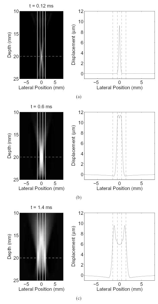
The axial displacement induced by radiation force from a pushing pulse of 5.3 MHz and focused at 20 mm is shown. On the left are images of the displacements, where the transducer is located at the top of the image, and lighter shades indicate greater displacement. On the right is a cross-section of the image taken at the focal point of the displacements. (a) Axial displacements 0.12 ms after force cessation. (b) Axial displacements after 0.6 ms elapsed. Shear waves are beginning to form, however they have not completely separated yet. (c) After 1.4 ms, the shear waves have completely separated and can be seen moving away from the location of force application.

Fig. 1(b) shows the displacement after an elapsed time of 0.6 ms. In this figure, a lateral broadening of the displacement region is seen. The broadening results from a cylindrical spreading of a shear wave as it propagates out from the region of excitation. On the right, displacement in the region of excitation is shown to be fairly flat in the center.

Fig. 1(c) shows the displacement 1.4 ms after the radiation force is applied. In this figure, two shear waves are visible traveling away from the initial push location, as one would see if a pebble were dropped in a pool of water, where the image is showing a cross-section of the wave. As the shear waves travel away from the initial push location, the region of displacement spreads out and the magnitude of displacement decreases. The attenuation of the shear wave is increased in materials or tissue that have viscoelastic properties.

In Fig. 1, the positions of four parallel beams are indicated by the solid white lines in the left images, and the dotted lines in the right images (the physical placement of parallel beams is exaggerated in these images for better visibility). In conventional ARFI imaging, the broadening of the localized displacement is ignored, and only the displacement in the center of the region of excitation is observed. The broadening of the push region is significant for parallel tracking in ARFI because the parallel beams are not placed directly over the center of the excitation region. The major noise source in the measurements of displacement with any tracking beam, however, is the amount of shearing within the tracking beam [12, 13], where shearing is the distortion of the original scatterer distribution [14–17].

III. METHODS

Simulations performed with finite element models (FEM) and Field II [18], and experiments in homogeneous phantoms were used to characterize the parallel tracking method for ARFI imaging. The simulation methods used here are identical to that described in [12], and are briefly summarized here. Model meshes for FEM simulations were created in Hyper-Mesh (Altair Computing Inc., Troy, MI) and imported into LS-DYNA3D (Livermore Software Technology Corporation, Livermore, CA) to solve the dynamic equations of motion for tissue displacement. Displacements determined in the FEM simulations were then used to model the displacement of scatterers in Field II. Image pulses created in Field II were then used to obtain rf signals before and after scatterer displacement.

A 5.3 MHz, commercial linear array (VF7-3, Siemens Medical Solutions USA, Inc., Issaquah, WA) was used with a SONOLINE Antares^TM scanner (Siemens Medical Solutions USA, Inc.) to perform conventional and parallel tracking for ARFI imaging in tissue mimicking phantoms. Both imaging methods were implemented by custom designed image sequences programmed into the Antares. The length of the acoustical pushing pulses was 37.5 μs. In-phase (I) and quadrature (Q) signals from the image sequence were acquired through the use of the Axius Direct^TM Ultrasound Research Interface (Siemens Medical Solutions USA, Inc.). Displacements were tracked at a rate of 8.4 kHz and measured using Loupas’ phase-shift estimator [19]. This phase-shift estimator offers high speed computation with jitter levels near that of cross-correlation [20].

A. Receive-Tracking Beam Position

Using a 4 kPa homogeneous phantom, focal point displacements were measured as a function of the offset between the transmit and receive foci of the tracking beam, and as a function of time. The phantom was a Computerized Imaging Reference Systems (CIRS) tissue-mimicking phantom (CIRS, Norfolk, VA) that was readily available and had well-characterized attenuation and sound velocity. The Young’s modulus of the CIRS phantom was measured to be 4 kPa using low-frequency compression testing with an MTS hydraulic actuator (MTS, Minneapolis, MN) [21]. The CIRS phantom has an ultrasonic attenuation of 0.7 dB/cm/MHz and a sound speed of 1540 m/s.

Simulations of the point spread function (PSF) were performed for the parallel tracking system with Field II. Transmit f-numbers (F/#) were varied between 1, 2, and 3, and a receive F/# was fixed at 0.5 in the simulations, where F/# is the ratio of the focal depth to the aperture width. The sidelobe level and positional error of the tracking-beam PSF was measured at the axial focus as a function of the receive-beam offset. For comparison, all experimental images were obtained with a transmit F/# of 2 and a receive F/# of 0.5.

B. Comparative Images

ARFI images comparing displacements observed with conventional and parallel tracking methods were generated from the CIRS phantom. Using conventional tracking for ARFI imaging (1:1 ratio), the tissue response from 96 push locations were observed with 96 tracking beams. The pushing locations were spaced 0.18 mm apart, which is similar to the beam spacing used for B-mode imaging.

Images also were generated from the CIRS phantom comparing 4:1, 8:1, and 12:1 parallel tracking. Because the Antares scanner is limited to 4 parallel-beamformed lines, the images formed with 8:1 and 12:1 tracking were formed synthetically from additional pushes at the same location. Although not formed from true parallel tracking, these images represent the capabilities of systems with 8:1 and 12:1 parallel tracking. Tracking-beam spacing was the same as in conventional tracking, however the spacing of the pushing beams were 0.71, 1.42, and 2.12 mm for the three parallel modes, respectively. A total of 96 locations were tracked for each of the parallel modes, however the number of pushing beams varied with the number of parallel tracked lines: 24 for 4:1, 12 for 8:1, and 8 for 12:1 tracking. The same 16.9 mm field-of-view was acquired with all three parallel tracking modes and the conventional tracking mode. Images were also generated of more clinically useful conventional and parallel ARFI images, where the spacing of the push locations for conventional tracking was 0.53 mm, and the parallel tracking mode used 4:1 parallel lines to track a region of size identical to that used in the 8:1 tracking mode (0.35 mm spacing between tracking beams).

The target in these images was a hard spherical inclusion with a 3 mm diameter, surrounded by a soft homogeneous region. This spherical inclusion had a Young’s modulus of approximately 31 kPa, giving the inclusion a mechanical contrast of 87% with the surrounding region The mechanical contrast is defined as one minus the ratio of the Young’s moduli of the two regions [22]. Image contrast of the lesion was measured as a function of time where contrast was computed as 1 −D_i=D_o, where D_i and D_o are the displacements inside and outside the lesion, respectively, and the sign of the contrast indicates whether the inner region is lighter or darker (i.e. greater or smaller displacement) than the surrounding region. When computing the contrast, two circular regions, 3 mm in diameter, were selected from the lesion and the background, where the two regions were adjacent laterally. Contrast-to-noise ratio (CNR) of the lesion was also measured as a function of time. CNR was measured as

$$\frac{\langle D_i\rangle -\langle D_o\rangle }{\sqrt{{\sigma }_i^2+{\sigma }_o^2}},$$ (5)

where ${\sigma }_i^2$ and ${\sigma }_o^2$ are the displacement variances of the regions inside and outside the lesion, respectively.

C. Material Stiffness

In equation 4, the velocity of the shear waves is shown to be proportional to the square root of the material’s stiffness. Therefore, the time required for the shear wave to propagate beyond the parallel tracked region will be shorter in stiff materials than in soft materials. To compare the effects of material stiffness on the parallel tracking method, FEM simulations of homogeneous regions were performed with Young’s moduli of 1, 5, 10, and 18 kPa, and the displacements recorded as a function of time for different offsets of the tracking beam.

D. Thermal Effects

Not all of the energy absorbed by the tissue produces a radiation force. The great majority of the energy is converted to heat. The amount of tissue heating from ARFI imaging using the parallel tracking method was compared to heating observed with conventional tracking using finite element simulations. A simulation of the tissue heating from a VF7-3 probe was performed using the heating model described in [8] and assuming 72 push locations spaced 0.53 mm apart and a focal depth of 2 cm. Tissue absorption was assumed to be 0.7 dB/cm/MHz, the thermal conductivity was assumed to be 6.0 mW/cm/°C, and the specific heat was assumed to be 4.2 J/cm³/°C. These thermal material properties are associated with generic soft tissue as specified in the NCRP Report #113 [23]. To interrogate an identical sized region using the parallel tracking method, 27 push locations with 1.42 mm spacing were required. The two imaging modes were compared with respect to their two-dimensional heating profiles for a single frame, 5 frames at the same frame rate, and imaging over 2.16 seconds at their maximum frame rates.

Heating of the transducer surface was measured experimentally for each of the conventional and parallel ARFI methods described above. To measure the heating at the patient/transducer interface, a type T thermocouple was placed between a VF7-3 transducer and the CIRS phantom. Ultrasound gel was used to provide coupling between the transducer and the phantom in accordance with IEC standards [9]. The ultrasound system was continuously running with conventional B-mode imaging in order to reach a steady state temperature for the transducer. Temperatures were recorded with a Quatech (Hudson, OH) data acquisition board before, during, and after ARFI imaging. Each imaging mode was run 10 times, and the mean temperature rise was computed from the stored temperature data.

IV. RESULTS

A. Receive Beam Position

Fig. 2 shows a surface plot of the displacements measured in a homogeneous 4 kPa phantom as a functions of the parallel-tracking beam offset (Δx) and observation time. Initially after pushing, a gradual decrease in measured displacement can be observed as the tracking beam is moved further from the region of excitation (Δx = 0). Although a sharp peak at might be expected at Δx = 0 and t = 0.12 ms, as seen in Fig. 1(a), results from Palmeri et al. [12] indicate that displacements measured by ultrasonic tracking for the experimental conditions here will underestimate the actual displacement by around 50%. As time progresses from the initial excitation, the measured displacements at all locations are growing due to inertia [24]. Propagating shear waves can be observed by the movement of the peak displacement over lateral space and time.

Fig. 2.

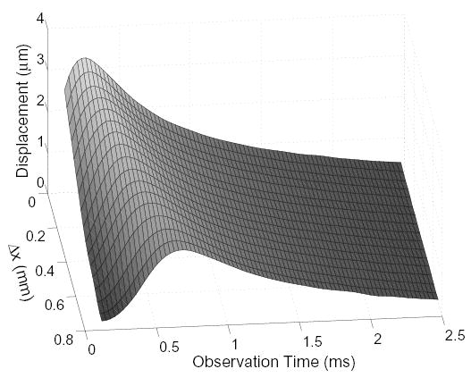
Measured displacement from a pushing pulse as a function of the parallel-tracking beam’s distance from the push location (Δx) and observation time in a homogeneous 4 kPa phantom.

The greatest displacement in Fig. 2 is observed when one of the parallel beams is directly over the push location. As the tracking beam moves further away, the measured peak displacement is smaller and occurs later in time. Regardless of parallel beam position, however, the displacements are nearly identical for all beams after reaching its peak in displacement. These results agree well with those shown by Sarvazyan et al. [1].

Fig. 3 shows the effect of laterally steering the tracking beam’s receive focus away from the transmit focus on the azimuthal PSF. The PSF of the beam used for conventional tracking has no offset and is symmetric. As the receive focus is shifted away from the transmit focus, the shape of the PSF becomes increasingly distorted and the sidelobes increase. The transmit F/# for these PSFs was 2, and the receive F/# was 0.5.

Fig. 3.

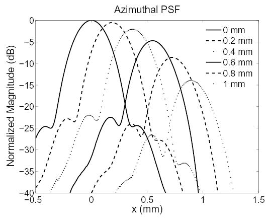
The azimuthal PSF for different offsets between the transmit and receive foci of the tracking beam. At an offset of 0 mm, the PSF is identical to that used in conventional tracking. All PSFs are normalized relative to the peak of the PSF with no offset.

In Fig. 4, the ratio of the sidelobe magnitude relative to the mainlobe and the positional error of the PSFs is shown as a function of offset. In these figures, the transmit F/# of the tracking beam is varied between 1, 2, and 3, and the receive F/# remains fixed at 0.5. In the left graph, it is clear that a low transmit F/# favors conventional tracking. For parallel tracking, a larger transmit F/# is favored because less shearing is introduced into the rf signals via the sidelobes, thereby minimizing the effect of jitter noise in the displacement estimates.

Fig. 4.

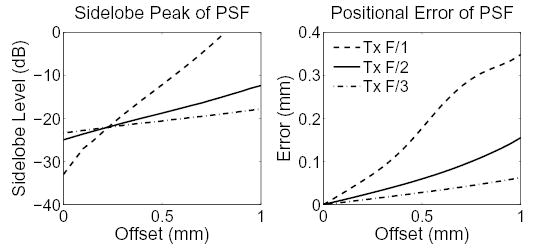
The sidelobe level (left) and positional error (right) of the PSFs as a function of offset between the transmit and receive foci of the tracking beam for three transmit beam f-numbers.

Because the tracking beam’s transmit and receive foci are different under parallel tracking, the position of the tracking beam PSF is shifted away from its ideal location, which is the receive focus. This positional error occurs because the transmit response asymmetrically weights the receive response of the PSF. The positional error is nonexistent when a plane wave is transmitted, however when the transmit pulse is more tightly focused, the positional error is greater. In the right graph of Fig. 4, the positional error of the PSF is plotted as a function of offset. The positional error of the PSF can adversely effect the shape and characteristics of the imaging target and may generate nonuniform lateral sampling of the target. For example, for a receive-beam offset of 0.6 mm, a transmit F/# of 1, and a receive F/# of 0.5, the positional error of the PSF is 0.23 mm. This error is greater than the beamspacing used in the images in Fig. 5. Therefore, it is clear from this figure that large transmit f-numbers are more favorable for parallel tracking.

Fig. 5.

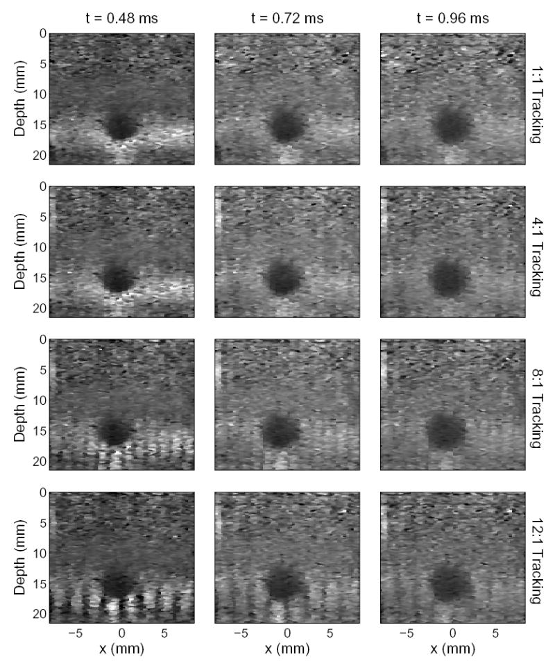
Images generated from the tissue mimicking phantom using conventional and 4:1, 8:1, and 12:1 parallel tracking. The images were produced 0.48 ms, 0.72 ms, and 0.96 ms after excitation. The images formed by 8:1 and 12:1 tracking were formed synthetically due to limitations of the Antares scanner, however they represent images that would be formed by systems with high parallel tracking capabilities.

B. Comparative Images

ARFI images comparing conventional and parallel tracking are shown in Fig. 5. The images were generated 0.48, 0.72, and 0.96 ms after pushing. Images generated by conventional ARFI tracking (1:1 Tracking) are shown in the top row. Images comparing 4:1, 8:1, and 12:1 parallel tracking with ARFI imaging are shown in the next three rows. The target is a hard spherical inclusion of 31 kPa at 15 mm depth, surrounded by a homogeneous 4 kPa region.

Depth dependent gain was applied to the image to improve image contrast over depth. In the first few time steps, the images are significantly different. For example, in the images generated by conventional and 4:1 tracking, a highly sampled image is observed with smooth transitions between pushing regions at 0.48 ms. In the images generated by 8:1 and 12:1 synthetic tracking, a grating artifact dominates the image. This grating artifact occurs because the shear waves have not propagated far enough to yield uniform displacement across the parallel tracked region in the homogeneous parts of the phantom. As time progresses, the grating artifact disappears as the shear waves propagate beyond the tracked regions. Therefore, at the later time steps, the images appear more like the conventional images. Although the 4:1 images do not show this grating artifact, it is present in earlier time steps not shown (at 0.12 and 0.24 ms, for example). The grating artifact does not appear in the near field because the push beam is much broader than the tracked region. Data acquisition time was 460 ms for the top row of images, 133 ms for 4:1 tracking, and 66 and 44 ms for 8:1 and 12:1 tracking assuming true parallel tracking.

The beam spacing used in B-mode imaging is difficult to achieve in conventional ARFI imaging because of significant heating of the transducer. Often a much larger beam spacing is used for conventional ARFI imaging. The left image in Fig. 6 shows the same target and field-of-view as in Fig. 5, however a beam spacing more typical to conventional ARFI imaging was used. In this figure, the image was produced by spacing the push lines every 0.53 mm. This image requires only 32 pushes to create the image, however the sample spacing is three times greater than previously.

Fig. 6.

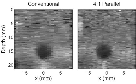
A conventional ARFI image created with 0.53 mm beam spacing is compared to a diagnostically useful parallel tracking scheme with 0.35 mm beam spacing (Note that the conventional image can be generated using 0.35 mm spacing as well, which will improve the spatial resolution, but at the cost of additional heating). These images were created 0.72 ms after application of radiation force.

The right image in Fig. 6 displays a diagnostically useful sampling scheme for a 4:1 parallel tracking method on the Antares. For this image, the push locations were spaced 1.42 mm apart and the tracking beams were spaced 0.35 mm apart. This configuration of the parallel beams covers the same sized region as 8:1 parallel tracking, however only half the number of tracking beams are used with twice the sample spacing. Data acquisition times for these two images were 153 ms with conventional tracking and 68 ms with parallel tracking.

The contrast of the spherical inclusion in figures 5 and 6 is shown in Fig. 7(a). The contrast for both conventionally tracked images in figures 5 and 6 is nearly identical, so only one set of data is shown for both images. The image created from 4:1 tracking with twice the spacing (Fig. 6) is labeled as ‘4:1 2x’ in Fig. 7. For all modes, a general decrease in contrast can be seen over the measured time period. The contrast of the lesion is nearly identical between all modes except the images generated from 12:1 tracking, which appear to have a little less contrast. The negative values of contrast indicate that reversal of lesion contrast is seen after 2 ms in all modes, consistent with Nightingale et. al [7]. Contrast reversal is caused by reverberating shear waves within the lesion [24].

Fig. 7.

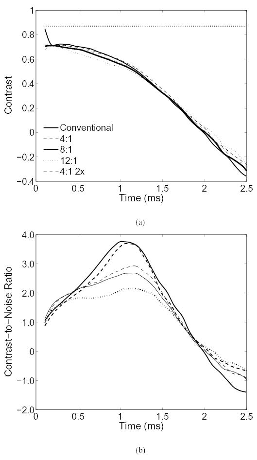
(a) The contrast of the lesion in figures 5 and 6 as a function of time. The mechanical contrast of the lesion, 87%, is shown by the horizontal dotted line. (b) The contrast-to-noise ratio of the lesion.

In Fig. 7(b), the CNR of the images is plotted as a function of time. All modes show a well defined peak in CNR, except the 12:1 tracking mode, occurring between 1 and 1.2 ms. Noise in ARFI images result from jitter in the displacement estimates and is exacerbated by shearing within the PSF. In the parallel receive modes, differences in displacement seen by offset receive beam locations (i.e. the grating artifact) and larger sidelobes in the PSF can also introduce noise. The negative values of the CNR indicate the reversal of contrast seen in Fig. 7(a).

C. Material Stiffness

Fig. 8 shows results of a simulation of the normalized displacement observed by parallel beams located 0.30 and 0.71 mm from the push location for materials with 1, 5, 10, and 18 kPa. As expected, the shear wave travels faster in the stiffer materials, as evidenced by the peak in the displacement curves earlier in time. For a real-time ARFI imaging system using parallel tracking, the optimal time to create an image is just as the shear wave has passed the outermost parallel beam, or just as the displacement begins to recover in these figures. The problem, then, for choosing the correct time to create an image has two degrees of freedom: the size of the parallel tracked region, and the stiffness of the imaging target.

Fig. 8.

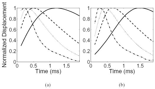
The simulated, normalized displacement observed by a parallel tracking beam located at an offset of (a) 0.30 mm and (b) 0.71 mm from the center of the push location. The elastic modulus for the homogeneous regions are 1 kPa (——), 5 kPa (– – –), 10 kPa (···· ), and 18 kPa (·–·–).

D. Thermal Effects

The temperature increase with conventional and parallel tracking techniques are compared in tissue with an absorption of 0.7 dB/cm/MHz in Fig. 9. The top row of images show heating associated with conventional ARFI imaging where 72 push locations, spaced 0.53 mm apart, are used per frame. The bottom row shows the heating associated with parallel ARFI techniques where 27 push locations are required per frame, spaced 1.43 mm apart.

Fig. 9.

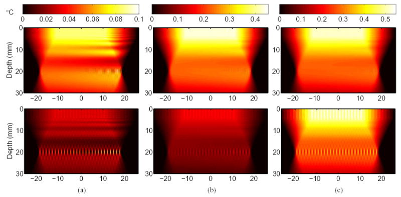
The temperature increase in tissue with an absorption of 0.7 dB/cm/MHz is compared for conventional and parallel tracking techniques. The color bar at the top of each column indicates the temperature increase in degrees Celsius. The top row of images show heating associated with conventional tracking and the bottom row shows the heating associated with 4:1 parallel tracking. The temperature change is shown for (a) a single frame, (b) 5 consecutive frames at the same frame rate (2.8 fps), and (c) 2.16 seconds at each mode’s maximum frame rate.

In Fig. 9(a) the temperature change is depicted for a single ARFI frame. The peak change in temperature for both imaging modes is 0.10°C, however the location of the peak is different for each mode. With conventional tracking, peaks occur at the focal point of the pushing pulses and near the surface of the transducer. Peak temperatures near the transducer surface result from the overlap of pushing pulses in the near field [8].

Because the push pulse is broad in the near field, the area absorbing ultrasonic energy overlaps significantly with neighboring push pulses. Therefore, even though the absorption of energy may be small in these areas, the cumulative effects of heating over many push pulses is great enough that a peak in heating may occur in the near field rather than at the focus [25].

For parallel tracking, the peak temperature increase occurs only at the focal point because there is less overlap between push pulses in the near field. In Fig. 9(b), the temperature change is shown for 5 consecutive ARFI frames, where both modes are executed at the same frame rate, 2.8 fps. For conventional tracking, the peak temperature change reaches 0.45°C close to the transducer, primarily due to push pulse overlap. With parallel tracking, the peak temperature change reaches 0.18°C at the focal point of the pushing pulses. Fig. 9(c) shows the temperature change over 2.16 seconds of imaging with each mode imaging at its maximum frame rate. This corresponds to 6 total frames at 2.8 fps with conventional tracking and 16 total frames at 7.4 fps with parallel tracking. The peak change in temperature in both imaging modes reaches 0.54°C, and occurs near the surface.

The measured changes in surface temperature of the transducer for each tracking mode is shown in table I. A single frame of conventional tracking, using the parameters applied in the tissue heating simulations, produced a surface temperature increase of 0.37°C. For a single frame of ARFI imaging using the parallel tracking technique, the frame rate more than doubles, but the amount of surface heating reduces to 0.17°C, or less than half of the original value. Five consecutive frames of conventional ARFI imaging produced a temperature increase of 1.70°C, compared to 0.63°C with parallel tracking at the same frame rate. If each mode is run for the same period of time at their respective maximum frame rates, conventional ARFI imaging yields an increase of 1.99°C over 2.16 seconds, while the parallel tracking method yields an increase of 1.68°C.

TABLE I.

MEAN CHANGE IN TRANSDUCER SURFACE TEMPERATURE

Imaging Mode	No. Frames	Frame Rate (fps)	Δ Temp. (°C) ± 1 s.d.
Conventional	1	2.8	0.37 ±0.01
Parallel	1	7.4	0.17 ±0.01
Conventional	5	2.8	1.70 ±0.01
Parallel	5	2.8	0.63 ±0.01
Conventional	6	2.8	1.99 ±0.03
Parallel	16	7.4	1.68 ±0.23

V. DISCUSSION

In conventional ARFI imaging, the imaging problem is straightforward in that the dynamic response of the tissue at the region of excitation is observed. This problem becomes more complex when parallel tracking is used to measure the response of the tissue because the region tracked by the parallel beams is often larger than the region of excitation. In this case, the shear waves generated by the excitation must pass into the tracked region before a valid image can be constructed.

It has previously been shown theoretically (for Gaussian shaped displacement fields and tracking beams) [13] and in finite element models [12] that for conventional tracking in ARFI imaging, displacement underestimation and jitter were minimized when the shearing within the PSF was minimized. In this case, the narrower the PSF, the more favorable the PSF is for tracking ARFI displacements. This is confirmed in Fig. 4 where the sidelobe levels are lowest for the narrowest tracking beam (transmit F/# 1, receive F# 0.5). The principle of the narrower PSF holds true for parallel tracking as well, however the choice for tracking beam F/#s may not be as obvious. Even though low F/#s produce narrower transmit and receive beams individually, the combined response of the system can be fairly broad when the transmit and receive beams are offset, as evident in the rapid rise in sidelobe level with offset. In the parallel tracking case, it is preferred to use a high transmit F/# and a low receive F/#. As this ratio increases, the sidelobes of the PSF contribute less and the positional error of the PSF decreases as shown in Fig. 4. Additionally, the low receive F/# maintains a narrow mainlobe.

There are several implications for parallel tracking in real-time ARFI imaging. First, the size of the tracking region and the elastic modulus of the material will affect the amount of time necessary for the shear waves to propagate far enough to create a useful image. Because the size of the tracked region is always known, it is simple to choose the appropriate time step based on the graphs shown in Fig. 8 for the given material stiffness. However, the elastic modulus of the material is unknown, and therefore user adjustment or, more likely, a conservative choice of temporal sample and/or receive-beam spacing is required in a real-time ARFI imaging system. For the imaging conditions in Fig. 2, this occurs in approximately 0.72 ms. Conversely, a broad pushing beam can be used to excite the tissue within the tracking region. This would eliminate the need for a long wait time if the region of excitation is the same size as the tracking region, because the shear velocity is independent of the size of the pushing beam. A broad pushing beam would also reduce displacement jitter. It is unrealistic, however, to produce pushing beams that have the same width as large tracking regions because the spatial resolution of the displacement images would be poor and severely diminish the contrast of imaging targets.

The fact that a wait time is necessary to produce an image is not necessarily detrimental to ARFI imaging using parallel tracking. For real-time ARFI imaging with conventional tracking, it is desirable to wait until the displacements increase along the axial extent of the image to allow the SNR to increase. For example, in the sequence of images in Fig. 5, a conventional real-time ARFI imaging system might use the image generated 0.48 ms after force application.

Although the contrast of a hard spherical lesion shown by the parallel tracking methods is nearly equivalent to the the contrast produced by conventional tracking methods, the CNR of the lesion suffers significantly as the size of the tracking region grows (Fig. 7). The loss in CNR is primarily due to degradation of the PSF, which increases the jitter in the displacement estimates.

Fig. 5 highlights the trade-off between contrast and tracking region size. Using 4:1 parallel tracking, the earliest time for which a reasonable image can be created is 0.48 ms for this imaging medium. This image shows the greatest contrast of the lesions, and the number of applied pushes are one-fourth the number used in conventional tracking. For 8:1 parallel tracking, the earliest an image can be created while minimizing grating artifacts is 0.72 ms. The contrast of this lesion is reduced compared to the 4:1 image at 0.48 ms, however the number of pushes is one-eighth the number used in conventional ARFI imaging. In the 12:1 tracking images, the earliest an image can be created is 0.96 ms after force cessation using one-twelfth the number of pushes used in conventional ARFI imaging. At this point in time, the contrast and overall image quality is significantly reduced. In particular, the lesion does not appear nearly as spherical as in the 4:1 and 8:1 images. This loss in quality can be attributed to poor coupling of the shear waves from the lesion into the background region, making the lesion appear larger than it really is. For more complete description of the dynamics of radiation force in lesions, the reader is referred to Palmeri et al. [24]. Poor coupling effects are more significant in the 12:1 tracking image because the pushes are spaced much farther apart, and the tracked regions are much larger. Shear waves attenuation may be greater in vivo than in tissue-mimicking phantoms, further increasing the expected grating and discontinuity artifacts seen in Fig. 5.

A strong motivation for parallel tracking in real-time ARFI imaging is the reduction in heat generated by the absorption of acoustical energy and generated by the transducer itself. Because parallel tracking requires fewer applications of force, less heat is generated (Fig. 9). Although the heat generated by a single frame is small, the heating effects become cumulative in real-time applications because the cooling time constants for the transducer and tissue are much slower than the rate of force application. For the same frame rates, parallel tracking generates less heat within the tissue than conventional tracking methods. In Fig. 9(c), the frame rate can be increased to 7.4 fps from 2.8 fps yet still retain the same heating characteristics as conventional ARFI imaging.

There is still concern, however, that the temperature rise is still significant after 2 seconds of imaging with the parallel mode. Optimization of the frame rate, the field-of-view, and the number of parallel beams used should improve the heating characteristics.

Considering contrast, CNR, the number of force applications, image artifacts, and heating, the parallel tracking mode that offers a reasonable compromise to all of these factors is the 8:1 tracking mode in a 2-D imaging system. Using the information from the 2-D system, it can be estimated that for a 3-D imaging system, 36:1 (in a 6 by 6 grid) can be used with the same spacing as used in the 2-D 8:1 system. The limiting factor for the 3-D system is the amount of distance covered in the diagonal of the 6 by 6 grid. This, of course, is assuming the system would be limited to rectangular grid. A more flexible system could incorporate additional parallel lines in a circular grid. Our current system is limited to 4:1 parallel tracking, so reasonable imaging parameters in this case would be to use the same size parallel tracking region as the 8:1 mode, but using half the sampling utilized in Fig. 6. This tracking mode shows similar contrast and noise characteristics to the 8:1 images (Fig. 7).

VI. CONCLUSIONS

We have demonstrated a parallel tracking method for acoustic radiation force impulse imaging. Parallel tracking of tissue displacements from radiation force was shown to produce images of quality almost identical to conventional tracking methods, provided that a wait time is imposed in order to allow the shear waves to propagate beyond the boundaries of the parallel tracked region. Because a proper wait time is already necessary for conventional tracking in real-time ARFI imaging, the addition of parallel tracking does not impose a significant loss in contrast of the imaging targets.

The optimal configuration for a parallel tracking system is a compromise of a number of factors including contrast, noise, size of the parallel tracked region, and heating. For our imaging conditions (4 kPa background and limited to 4:1 parallel tracking), a close-to-optimal configuration for a real-time ARFI imaging system would use 4:1 parallel tracking with lateral sampling equivalent to 2 times that of B-mode imaging and a wait time of 0.72 ms.

Heating issues are of a major concern to real-time ARFI imaging systems. Parallel tracking offers an option to either increase frame rate or decrease heating compared to conventional tracking methods. At the optimal parallel configuration for our system, heating was shown to be 2.5 times smaller in tissue and 2.7 times smaller at the transducer surface while maintaining the same frame rate as conventional ARFI imaging. For nearly the same amount of heat generation in tissue (a little less at the transducer surface), the frame rate could be increased by a factor of 8/3 for diagnostically useful imaging configurations.

References

- 1.Sarvazyan AP, Rudenko OV, Swanson SD, Fowlkes JB, Emelianov SY. Shear wave elasticity imaging: A new ultrasonic technology of medical diagnostics. Ultrasound Med Biol. 1998;24(9):1419–1435. doi: 10.1016/s0301-5629(98)00110-0. [DOI] [PubMed] [Google Scholar]
- 2.Walker WF, Fernandez FJ, Negron LA. A method of imaging viscoelastic parameters with acoustic radiation force. Physics Med Biol. 2000;45(6):1437–1447. doi: 10.1088/0031-9155/45/6/303. [DOI] [PubMed] [Google Scholar]
- 3.Fatemi M, Greenleaf JF. Vibro-acoustography: An imaging modality based on ultrasound-stimulated acoustic emission. Proc Natl Acad Sci USA. 1999;96(12):6603–6608. doi: 10.1073/pnas.96.12.6603. [DOI] [PMC free article] [PubMed] [Google Scholar]
- 4.Bercoff J, Tanter M, Fink M. Supersonic shear imaging: A new technique for soft tissue elasticity mapping. IEEE Trans Ultrason, Ferroelect, Freq Contr. 2004;51(4):396–409. doi: 10.1109/tuffc.2004.1295425. [DOI] [PubMed] [Google Scholar]
- 5.Nightingale KR, Soo MS, Nightingale RW, Trahey GE. Acoustic Radiation Force Impulse imaging: In vivo demonstration of clinical feasibility. Ultrasound Med Biol. 2002;28(2):227–235. doi: 10.1016/s0301-5629(01)00499-9. [DOI] [PubMed] [Google Scholar]
- 6.Sharma AC, Soo MS, Trahey GE, Nightingale KR. Acoustic Radiation Force Impulse imaging of in vivo breast masses; Proc IEEE Ultrason Symp; 2004. pp. 728–731. [Google Scholar]
- 7.Nightingale K, Palmeri M, Trahey GE. Analysis of contrast in images generated with transient acoustic radiation force. Ultrasound Med Biol. 2006;32(1):61–72. doi: 10.1016/j.ultrasmedbio.2005.08.008. [DOI] [PubMed] [Google Scholar]
- 8.Palmeri ML, Nightingale KR. On the thermal effects associated with radiation force imaging of soft tissue. IEEE Trans Ultrason, Ferroelect, Freq Contr. 2004;51(5):551–565. [PubMed] [Google Scholar]
- 9.IEC Standard 60601-2-37. Medical electrical equipment - particular requirements for the safety of ultrasonic medical diagnostic and monitoring equipment. International Electrotechnical Commission, Tech Rep. 2001 [Google Scholar]
- 10.Food and Drug Administration. Centre for Devices and Radiological Health, “Information for manufacturers seeking marketing clearance of diagnostic ultrasound systems and transducers. [Sept. 1997];US Department of Health and Human Services, Tech Rep. www.fda.gov/cdrh/ode/ulstran.pdf.
- 11.Shattuck DP, Weinshenker MD, Smith SW, von Ramm OT. Explososcan: A parallel processing technique for high speed ultrasound imaging with linear phased arrays. J Acoust Soc Am. 1984;75(4):1273–1282. doi: 10.1121/1.390734. [DOI] [PubMed] [Google Scholar]
- 12.Palmeri ML, McAleavey SA, Trahey GE, Nightingale KR. Ultrasonic tracking of acoustic radiation force-induced displacements in homogeneous media. IEEE Trans Ultrason, Ferroelect, Freq Contr. 2006;53(7):1300–1313. doi: 10.1109/tuffc.2006.1665078. [DOI] [PMC free article] [PubMed] [Google Scholar]
- 13.McAleavey SA, Nightingale KR, Trahey GE. Estimates of echo correlation and measurement bias in acoustic radiation force impulse imaging. 2003;50(6):631–641. doi: 10.1109/tuffc.2003.1209550. [DOI] [PubMed] [Google Scholar]
- 14.Embree PM, O’Brien WD. Volumetric blood flow via time-domain correlation: Experimental verification. IEEE Trans Ultrason, Ferroelect, Freq Contr. 1990;37(3):176–189. doi: 10.1109/58.55307. [DOI] [PubMed] [Google Scholar]
- 15.Bilgen M, Insana MF. Error analysis in acoustic elastography. II. Strain estimation and SNR analysis. J Acoust Soc Am. 1997;101(2):1147–1154. doi: 10.1121/1.418019. [DOI] [PubMed] [Google Scholar]
- 16.Friemel B, Bohs L, Nightingale K, Trahey G. Speckle decorrelation due to two-dimensional flow gradients. IEEE Trans Ultrason, Ferroelect, Freq Contr. 1998;45(2):317–327. doi: 10.1109/58.660142. [DOI] [PubMed] [Google Scholar]
- 17.Céspedes EI, de Korte CL, van der Steen AFW. Echo decorrelation from displacement gradients in elasticity and velocity estimation. IEEE Trans Ultrason, Ferroelect, Freq Contr. 1999;46(4):791–801. doi: 10.1109/58.775642. [DOI] [PubMed] [Google Scholar]
- 18.Jensen JA. Field: A program for simulating ultrasound systems. Med Biol Eng Comp, col 10th Nordic-Baltic Conference on Biomedical Imaging. 1996;4(1):351–353. [Google Scholar]
- 19.Loupas T, Peterson R, Gill R. Experimental evaluation of velocity and power estimation for ultrasound blood flow imaging, by means of a two-dimensional autocorrelation approach. IEEE Trans Ultrason, Ferroelect, Freq Contr. 1995;42:689–699. [Google Scholar]
- 20.Pinton GF, Dahl JJ, Trahey GE. Rapid tracking of small displacements with ultrasound. IEEE Trans Ultrason, Ferroelect, Freq Contr. 2006;53(6):1103–1117. doi: 10.1109/tuffc.2006.1642509. [DOI] [PubMed] [Google Scholar]
- 21.Palmeri ML, Sharma AC, Bouchard RR, Nightingale RW, Nightingale KR. A finite element method model of soft tissue response to impulsive acoustic radiation force. IEEE Trans Ultrason, Ferroelect, Freq Contr. 2005;52(10):1699–1712. doi: 10.1109/tuffc.2005.1561624. [DOI] [PMC free article] [PubMed] [Google Scholar]
- 22.Ponnekanti H, Ophir J, Huang Y, Cespedes I. Fundamental mechanical limitations on the visualization of elasticity contrast in elastography. Ultrasound Med Biol. 1995;21(4):533–543. doi: 10.1016/0301-5629(94)00136-2. [DOI] [PubMed] [Google Scholar]
- 23.NCRP, Report No. 113. Exposure Criteria for Medical Diagnostic Ultrasound. I. Criteria Based on Thermal Mechanisms. 1992. NCRP Publications, Bethesda, MD 20814: National Council on Radiation Protection and Measurements. [Google Scholar]
- 24.Palmeri ML, McAleavey SA, Fong K, Trahey GE, Nightingale KR. Dynamic mechanical response of spherical inclusions to impulsive acoustic radiation force excitation. IEEE Trans Ultrason, Ferroelect, Freq Contr. 2006 doi: 10.1109/tuffc.2006.146. (accepted) [DOI] [PMC free article] [PubMed] [Google Scholar]
- 25.O’Brien WD, Jr, Yang Y, Simpson DG. Evaluation of unscanned-mode soft-tissue thermal index for rectangular sources and proposed new indices. Ultrasound Med Biol. 2004;30(7):965–972. doi: 10.1016/j.ultrasmedbio.2004.03.015. [DOI] [PubMed] [Google Scholar]