Analyzing Chromatin Remodeling Complexes Using Shotgun Proteomics and Normalized Spectral Abundance Factors

Abstract

Mass spectrometry based approaches are commonly used to identify proteins from multiprotein complexes, typically with the goal of identifying new complex members or identifying post translational modifications. However, with the recent demonstration that spectral counting is a powerful quantitative proteomic approach, the analysis of multiprotein complexes by mass spectrometry can be reconsidered in certain cases. Using the chromatography based approach named multidimensional protein identification technology, multiprotein complexes may be analyzed quantitatively using the normalized spectral abundance factor that allows comparison of multiple independent analyses of samples. This study describes an approach to visualize multiprotein complex datasets that provides structure function information that is superior to tabular lists of data. In this method review, we describe a reanalysis of the Rpd3/Sin3 small and large histone deacetylase complexes previously described in a tabular form to demonstrate the normalized spectral abundance factor approach.

1. Introduction

A powerful approach to understanding the function of any given transcriptional protein is to determine its interaction partners. Proteomic analysis of protein complexes has facilitated the discovery of functional information about the roles of genes and their protein products in the biology of organisms from S. cerevisiae to humans. Directly incorporating generic affinity purification tags into individual genes simplified the analysis of protein complexes by mass spectrometry. For example, the tandem-affinity purification (TAP) tag [1] enabled the analysis of protein complexes in yeast including a large scale qualitative analysis of protein complexes from S. cerevisiae cells grown in YPD media [2]. Another notable report of a high-throughput protein complex identification is the study by Ho et al., which also analyzed protein complexes from S. cerevisiae grown in YPD media [3] using the FLAG epitope tag [4]. However, neither method proved sufficiently comprehensive to provide full coverage, and 50% of the data reported in these two high throughput proteomic analyses [2, 3] were predicted to be spurious [5]. Notably, high throughput analysis of protein complexes without consideration of the biology of the system and appropriate validation of interactions can lead to many false positives [5]. Finally, the data in both of these datasets is strictly qualitative. Alterations in abundance and content of protein complexes are key cellular events in response to stimuli. The lack of analysis of the dynamics of protein complexes from organisms in response to stimuli results from the lack of methodologies and technologies. With the advent of quantitative proteomics methods, this will change.

A powerful approach for analyzing the content of protein complexes is combining affinity purification via tagging of specific subunits with chromatography-based shotgun proteomics. Multidimensional protein identification technology (MudPIT) was originally devised as an approach for comprehensive analyses of proteomes [6, 7], but has proven even more powerful for the analysis of multiprotein complexes [8–10]. In a MudPIT analysis of a multiprotein complex, the complex is first purified—by either affinity chromatography, co-immunoprecipitation or traditional biochemical techniques—, then digested into peptides. Peptide mixtures are loaded onto a microcapillary column that serves as an electrospray ionization source when placed in line with an HPLC and a tandem mass spectrometer. The microcapillary column consists of three phases, reversed phase (RP), strong cation exchange (SCX), and reversed phase. Sample is desalted directly on the column in the first RP, after which a RP gradient moves peptides to the SCX portion of the triphasic column. Next, a salt pulse consisting of a low amount of ammonium acetate releases small batches of peptides from the SCX to the RP, and a RP gradient over 90 minutes elutes peptides into a tandem mass spectrometer. Iterative cycles of increasing salt concentration followed by RP gradients slowly elute peptides into the tandem mass spectra spectrometer where they are isolated and fragmented. The SEQUEST algorithm interprets the peptide sequence within tandem mass spectra [11], after which additional algorithms recombine thousands of peptides to determine which proteins were present in the original sample [12].

Typically, protein mass spectrometry analyses of multiprotein complexes results in a tabular list of the proteins present in the sample compared to a negative control. However, the number of peptides identified per protein is growing in use for quantitative analysis [13–20]. The most straightforward implementation of this approach is spectrum counting which is the total number of peptides used to identify a protein [13, 16, 19, 20]. An important consideration with spectrum counting and similar approaches is the fact that small proteins tend to have fewer peptides identified per protein compared to large proteins. Therefore, it is important to take into consideration the length [15] or sequence [18] of a protein when determining protein abundances using spectrum counting. We have recently expanded the spectrum counting approach to allow for normalization of spectrum counting data using normalized spectral abundance factor (NSAF) [21]. In this method article, we will revisit the analysis of the Large and Small Rpd3/Sin3 histone deacetylase complexes we recently described qualitatively in a tabular form [10, 22]. In the current body of work, we describe the purification and MudPIT analysis of these complexes, and we demonstrate that the NSAF approach is providing additional functional insight into protein complexes than previously obtained using tabular displays of protein lists.

2. Purification of Protein Complexes

2.1 Cell growth and extraction

Tandem affinity purification (TAP) tagged Rpd3 and Sin3 proteins in the S. cerevisiae cell line BY4741 are used as an example in this study. The entire S. cerevisiae TAP tag library is available from Open Biosystems (Huntsville, AL). A given yeast strain was inoculated into 5ml of YPD media (1% yeast extract, 1% peptone, and 2% glucose) overnight at 30°C. The following morning, 5ml of overnight media was added to 2.5L of YPD and grown in independent cultures of until reaching an optical density at 600nm of approximately 1.5 Cells were collected by centrifugation for 20 minutes at 4000 × g 4°C. The supernatant was discarded and the pellet was resuspended in 250 ml of cold ultrapure water followed by an additional centrifugation for 20 min at 4000 × g at 4°C for pelleting the cells. Again, the supernatant was discarded. Cells were resuspended in 25 ml of Extraction Buffer (40 mM HEPES-KOH (pH 7.5); 10 % glycerol; 350mM NaCl; 0.1 % Tween-20; with freshly added 1 ug/ml pepstatin A, 2 ug/ml leupeptin, 0.5 mM DTT, 1 mM PMSF) followed by centrifugation for 20 min at 4000 × g at 4°C. The supernatant was discarded and the cells resuspended in 25ml of Extraction Buffer with the centrifugation and resuspension in extraction buffer repeated a total of three times.

After the final resuspension of cells in 25 ml of Extraction Buffer, cells were broken open by using a bead beater model 1107900 (BioSpec Products Inc., Bartlesville, OK). Following this protocol, cells were disrupted with 25 ml of silica beads 0.5 mm diameter (BioSpec Products Inc., Bartlesville, OK) by rotating at high speed forces (0.43 HP motor) in a polycarbonate chamber of 50ml cooled with an ice water cooling jacket (BioSpec Products Inc., Bartlesville, OK). Ten cycles of 30 seconds bead beating and 1 minute break were performed. Beads were then washed with 10 ml of extraction buffer and the washed fraction added to the lysate. Next, beads and cell debris were spun down by centrifugation for 30 min at 4000 × g at 4°C. After transferring the supernatant to ultracentrifuge tubes, the supernatant was spun for 1.5 h at 45000 × g at 4°C. The supernatant contained the soluble protein extract and was used for further purification. The pellet contained membranes and unbroken cells and can be kept for additional experimentation or discarded.

2.2 Tandem Affinity Purification

The next step was binding the TAP tagged proteins to IgG Sepharose 6 Fast Flow (GE Healthcare, Piscataway, NJ). First, 500 μl of IgG resin was washed by centrifugation with 5 ml of extraction buffer followed by centrifugation for 2 min at 2000 × g at 4°C. This process was repeated three times. The clarified cellular protein extract was mixed with the washed IgG resin and incubated overnight at 4°C on a mixer. On the following day, the extract plus resin was transferred to 20 ml Poly-prep Chromatography columns (Biorad, Hercules, CA), and the extract was allowed to drain by gravity. Beads were washed with 20 ml of extraction buffer and drained by gravity. Next, beads were washed with 10 ml of TEV cleavage buffer (10 mM Tris (pH 8); 150 mM NaCl; 0.1 % NP-40; 0.5 mM EDTA; 10 % glycerol; with freshly added 1 ug/ml pepstatin A, 2 ug/ml leupeptin, 1 mM DTT, 1 mM PMSF) by gravity flow. Beads were then resuspended in the column with 1 ml of TEV cleavage buffer followed by transfer to a 1.5 ml microfuge tube. After adding 10 ul of AcTEV protease (Invitrogen, Carlsbad, CA), the tubes were incubated overnight at 4°C on the mixer.

The following day, the suspension was transferred in a new 20ml column and the TEV cleaved products were eluted by allowing the buffer to drip out of the column by gravity. The resin was washed with 3 ml of calmodulin binding buffer 0.3 M (10 mM Tris (pH 8); 1 mM MgAc; 1 mM Imidazole; 2 mM CaCl₂; 0.1 % NP-40; 10 % glycerol; 0.3 M NaCl; with freshly added 1 ug/ml pepstatin A, 2 ug/ml leupeptin, 0.5 mM DTT, 1 mM PMSF). This flow through was pooled with the fraction containing the TEV cleaved products. To the TEV cleaved products and the washing fraction were added 3 μl of 1M CaCl₂. Next the Calmodulin Sepharose 4B resin was washed (GE Healthcare, Piscataway, NJ) by centrifugation with 5 ml of Calmodulin binding buffer 0.3 M NaCl. This procedure was carried out three times. After washing, the TEV cleaved products were mixed with the Calmodulin resin and incubated overnight at 4°C on mixer.

The following day, the resin was washed by centrifugation 5 min at 2000 × g at 4°C in five successive steps. The first three washes were with calmodulin binding buffer NaCl 0.3 M followed by two washes with calmodulin binding buffer NaCl 0.15 M (10 mM Tris (pH 8); 1 mM MgAc; 1 mM Imidazole; 2 mM CaCl₂; 0.1 % NP-40; 10 % glycerol; 0.15 M NaCl; with freshly added 1 ug/ml pepstatin A, 2 ug/ml leupeptin, 0.5 mM DTT, 1 mM PMSF). After transferring the resin to a 1.5ml microfuge tube, 500 μl of calmodulin elution buffer (10 mM Tris (pH 8); 0.15 M NaCl; 1 mM MgAc; 1 mM Imidazole; 2 mM EGTA; 0.1 % NP-40; 10 % glycerol; with freshly added 1 ug/ml pepstatin A, 2 ug/ml leupeptin, 0.5 mM DTT, 1 mM PMSF) were added and mixed for 5 minutes at room temperature. Next, the resin was spun down by centrifugation for 1 min at 14000 × g at 4°C and the supernatant was transferred in a clean tube. This elution step was repeated nine times and each of the elution fractions was analyzed by SDS-PAGE using silver staining (Figure 1).

Figure 1. Purification of Rpd3/Sin3 Large and Small Complexes.

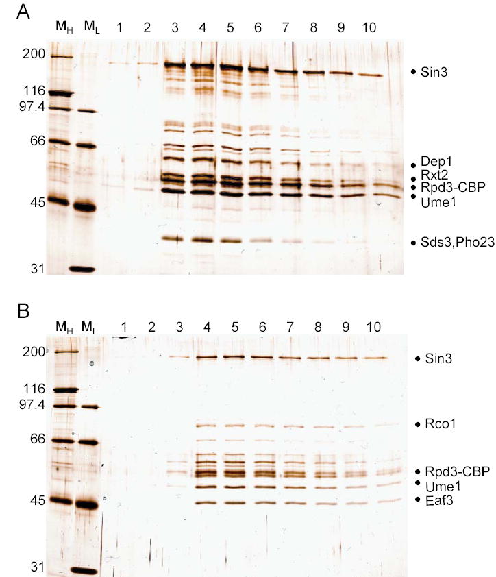
Whole cell extracts (section 2.1) from 6L of the RPD3-TAP strain culture were subjected to Ig-Sepharose followed by TEV elution (section 2.2). TEV eluates were fractionated on MonoQ ion exchange chromatography to separate the small and large Rpd3/Sin3 complexes (section 2.3). A. MonoQ fractions 26 through 30 corresponding to Rpd3/Sin3L (as defined by Superose 6 gel filtration, [10]) were pooled and further subjected to Calmodulin-sepharose. EGTA elutions 1 through 10 were resolved on 8% SDS-PAGE followed by silver staining. Bands known to correspond to different subunits are shown. B. MonoQ fractions 19 through 23 containing Rpd3/Sin3S were pooled and further subjected to Calmodulin-sepharose. EGTA eluates 1 through 10 were resolved on 8% SDS-PAGE followed by silver staining. Bands known to correspond to different subunits are shown.

2.3 Fractionation of large and small Rpd3/Sin3 complexes

In many circumstances, the TAP purification followed by protein mass spectrometry is insufficient to completely characterize multiprotein complexes. In the case of the example used in this article, Rpd3 and Sin3 belong to large and small Rpd3/Sin3 complexes, each with distinct subunit compositions and functions [10, 22]. When planning on separating the large and small Rpd3/Sin3 complexes, it is recommended to grow at least 6L of YPD cultures at optical density at 600nm of approximately 1.5, because the additional chromatography step will lead to sample loss. In order to separate large (Rpd3L) and small (Rpd3S) complexes, the following change to the TAP purification protocol described above was made.

The TEV cleavage eluate was applied to a 1ml MonoQ anion-exchange column at 4°C. The large and small Rpd3/Sin3-containing complexes were eluted using a linear gradient ranging from 0.1 M NaCl to 0.5 M NaCl in 50 mM Tris-HCl, pH 8, 10% glycerol, 0.1% Tween-20, 1mM PMSF, and 0.5mM DTT. The fractions were analyzed using western blotting with the anti-TAP antibody (Open Biosystems, Huntsville, AL) to determine the fractions containing the small and large Rpd3/Sin3 complexes. The small complex eluted before the large complex on a MonoQ column and two to three fractions containing each form of the complex were pooled and subjected to the calmodulin binding and EGTA elution steps described above.

Six different samples were obtained and subjected to MudPIT analysis: whole TAP fractions from Rpd3-TAP and Sin3-TAP cells, large/small complexes purified from Rpd3-TAP, and large/small complexes purified from Sin3-TAP.

3. Analysis of multiprotein complexes by MudPIT

3.1 Protein digestion

The protein eluates were first TCA precipitated by bringing the solution to 400μ1 with 100mM Tris-HCl, pH 8.5, and adding 100μl 100% Trichloroacetic Acid (final TCA concentration of 20%). The reaction was carried out on ice and the sample was left overnight at 4°C. The following day, the TCA-precipitated proteins were pelleted down by centrifugation at 14,000 rpm for 30min at 4°C. The supernatant was drawn with a gel loading tip, leaving 5 to 10μl in the tube such as not to disturb the pellet. Next, the protein pellet was washed twice with 500 μl of cold acetone followed by centrifugation for 10 minutes at 14,000 rpm in a microfuge. Lastly, the acetone washed pellet was dried using a speed vac for 5 minutes.

Next, 100mM Tris-HCl, pH 8.5, 8M Urea (freshly made) were added to the TCA-precipitated proteins and vortexed until the sample was in solution. The solution was brought to 5mM Tris (2-Carboxylethyl)-Phosphine Hydrochloride (TCEP) with 0.1M stock solution, and incubated at room temperature for 30 min. Iodoacetamide was added to 10 mM IAM with 0.5M stock, and the carboxyamidomethylation was let to proceed at room temperature in dark for 30 min. Endoproteinase LysC (Roche Applied Science, Indianapolis, IN) was added at 1 μg/μl (1:100) to the denatured, reduced, and carboxymethylated proteins; and incubated at 37°C for at least 6 hours. After endoproteinase LysC digestion, the solution was diluted to 2M Urea with 100mM Tris-HCl, pH 8.5, and CaCl₂ was added to 2mM from a 500mM stock solution. Finally, trypsin (modified sequence grade, Roche Applied Science, Indianapolis, IN) was added at 0.1 μg/μl (1:100), the digestion was let to proceed at 37°C overnight while shaking. On the next day, 90% Formic acid was added to 5% and the sample stored at −80°C.

3.2 Microcapillary Column Construction and Sample Loading

Three phase microcapillary columns were used for all analyzed peptide mixtures [23]. To begin, a window was burnt in the center of ~50 cm of 100 μm × 365μm fused silica capillary (Polymicro Technologies, Phoenix, AZ) by holding it over a flame until the polyimide coating has been charred. The charred material was removed by gently wiping the capillary with a tissue soaked in methanol. Next, to pull a needle, the capillary was placed into a Model P-2000 Laser Puller (Sutter Instrument Co. Novato, CA), with the capillary exposed window positioned in the mirrored chamber. Our 4 step parameter setup for pulling ~3 to 5 μm tips from a 100 μm i.d. × 365 μm o.d. capillary was as follows: [Heat = 290, Velocity = 40, and Delay = 200], [Heat = 280, Velocity = 30, and Delay = 200], [Heat = 270, Velocity = 25, and Delay = 200], and [Heat = 260, Velocity = 20, and Delay = 200], with all other values set to zero.

Next, triphasic columns (one for each peptide mixture) were packed in the pulled microcapillaries. First, 15 to 20 mg of Aqua Reversed Phase (RP) (Phenomenex, Torrance, CA) packing material was mixed with 1 mL of MeOH into a 1.7 ml microfuge tube, and the resulting slurry was placed into a stainless steel pressurization vessel (Brechbuehler, Inc., Houston, TX, or materials transfer agreement for blueprints available by request from John Yates, Scripps Research Institute, La Jolla, CA).. The pulled microcapillary column was inserted into a Swagelok^® fitting with a 0.4 mm Teflon ferrule in the lid of the pressure vessel and fed through the ferrule until the end of the capillary reached the bottom of the microfuge tube. Helium pressure was then applied to 500 to 1000 psi to push the packing material up into the pulled microcapillary, until the RP level was about 9 cm from the top of the column. Similarly, a slurry of 15 to 20mg/ml Whatman Paritshpere SCX (Whatman, Florham Park, NJ) was prepared in methanol, and packed in the same microcapillary until the SCX level was about 3 cm below the first RP level. Finally, the microfuge tube with RP in methanol was placed back into the pressurization vessel and another 2 cm of RP material was added after the SCX.

The packed column was washed with methanol for at least 10 min, and equilibrated with Buffer A (5%ACN, 0.1% formic acid) for at least 30 min. To get rid of any particulate (which could clog the microcapillary column), the peptide mixture to be loaded was spun down for 30 min at 14,0000 rpm and the supernatant transferred to a new 1.7ml microfuge tube using a gel loading tip. The peptide mixture was then loaded by placing the 1.7ml microfuge tube into the pressurization vessel. The loaded column was washed with Buffer A for at least one hour until installed onto the mass spectrometer.

3.3 Liquid Chromatography coupled to Tandem Mass Spectrometry

The loaded and washed three phase column was installed onto a nano electrospray stage (MTA for blueprints available by request from John Yates, Scripps Research Institute, La Jolla, CA). This nanoelectrospray stage was coupled to a Agilent 1100 series G1379A degasser, G1311A quaternary pump, G1329A autosampler, G1330B autosampler thermostat, and G1323B controller (Agilent Technologies, Palo Alto, CA) and an LCQ DECA-XP^plus tandem mass spectrometer (Thermo Electron, San Jose, CA) [24]. The HPLC flow rate was kept constant at 0.1 ml/min throughout the chromatography. However, to achieve a flow rate at the tip of the column of about 200–300 nl/min, the flow was split using a waste line consisting of 50 μm fused silica capillary cut to about 40 cm. The microcapillary column, quaternary HPLC pump, overflow tubing, and gold wire (through which a 2.4 kV voltage was applied) were connected using a MicroTight Cross (Upchurch).

The gradient profile used for analyzing protein complexes was set-up through and controlled by the Xcalibur^™ instrument software. Since we used three phase columns [23], the first step was a reversed phase gradient to move any bound peptide from the first RP to the SCX material. Then, successive salt bumps were run to move small amounts of peptides from the SCX onto the last RP, followed by a slow reversed phase gradient to resolve peptides within the last RP before they were eluted off into the mass spectrometer. The three buffers were buffer A (5% Acetonitrile, 0.1% formic acid made with HPLC grade water), buffer B (80% Acetonitrile, 0.1% formic acid made with HPLC grade water), and buffer C (500 mM Ammonium Acetate, 5% Acetonitrile, 0.1% formic acid made with HPLC grade water). The gradient profile of the first step was a 16 minute linear gradient from 0 to 60% Buffer B followed by a 1 minute linear gradient to 100% Buffer B, with three minutes at 100% Buffer B for a total time of 20 minutes. The gradient profiles of the next four chromatographic steps began with 3 minutes of 100% Buffer A followed by 2 minutes of X% Buffer C (where X was equal to 15, 30, 50, and 70% in step 2, 3, 4, and 5, respectively), followed by 100% Buffer A for 5 minutes, followed by a 15 minute linear gradient to 15% Buffer B, followed by a 92 minute slow linear gradient to 45% Buffer B for a total time of 117 minutes. The gradient profile of the final step began with 2 minutes of 100% Buffer A, followed by 20 minutes of 100% Buffer C, followed by 5 minutes of 100% Buffer A, followed by a 10 minute linear gradient to 20% Buffer B, followed by a 48 minute linear gradient to 70% Buffer B, followed by a 5 minute linear gradient up to 100% Buffer B, which is then held at 100% Buffer B for 5 minutes, ending with 2 minutes at 100% Buffer A for a total time of 97 minutes.

Data dependent acquisition of tandem mass spectra during the HPLC gradient was programmed through the LCQ Xcalibur^™ software. The method consisted of a continual cycle beginning with one MS scan, which recorded all of the m/z values of the ions eluting into the mass spectrometer at a particular point in time, followed by three rounds of MS/MS at 35% collision energy. Full MS spectra were recorded on the peptides over a 400 to 1,600 m/z range. Dynamic exclusion was activated to improve the protein identification capacity during the analysis. Extended details regarding the instrumentation setup have been described previously [24].

Upon the completion of a run, *.RAW files which have been acquired by the mass spectrometer were converted to *.DAT files for MS/MS analysis using the XCalibur file converter function. An example of the chromatographic profile of a successful analysis is shown in Figure 2 where the six step MudPIT analysis described above was used to analyze the large Rpd3/Sin3 complex purified using the Sin3-TAP strain and the purification procedure described in section 2.1.

Figure 2. Base Peak Chromatograms from a MudPIT Analysis of Rpd3/Sin3L.

A peptide mixture generated from Rpd3/Sin3L (section 3.1) obtained from affinity and MonoQ purifications of Sin3-TAP was resolved on a triphasic microcapillary column (section 3.2) using the six step multidimentional gradients described in section 3.3.

4. Data Analysis

4.1 MS/MS dataset Search

Each dat file was converted into a ms2 file [25] using extract-ms in order to obtain the coordinates of the MS/MS spectra to be analyzed. Each ms2 file was then subjected to the 2to3 software [26] to remove spectra of poor quality and assign a tentative charge state to precursor peptides.

SEQUEST™ [11] was used to search the ms2 files against a database containing Saccharomyces cerevisiae protein sequences downloaded from the National Center for Biotechnology Information (NCBI). This database consisted of 5872 S. cerevisiae sequences (NCBI, March 6^th, 2006 release), complemented with 177 sequences from usual contaminants such as human keratins, IgGs, and proteolytic enzymes. In addition, to estimate false positive discovery rates (FDR), each sequence was randomized (keeping the same amino acid composition and length), and the resulting 6049 “shuffled” sequences were added to the “normal” yeast database and searched at the same time [27]. For every spectrum matching a “shuffled” peptide, there should be one false positive in the “normal” dataset. The Peptide False Discovery Rate (FDR) was hence calculated based on spectral count (SpC) as in [28]:

$$\text{FDR}=\frac{(2\times \text{"Shuffled"\_SpC})}{\text{Total\_SpC}}$$ (eq. 1)

The sequest.params file was set up such as the peptide mass tolerance was 3; no enzyme specificity was required; parent ions were calculated with average masses, while fragment ions were modeled with monoisotopic masses; and cysteine residues were considered fully carboxyamidomethylated (+57Da) and searched as a static modification.

4.2 Protein list assembly and comparison

DTASelect [12] was used to parse the peptide information contained in the SEQUEST output files and assemble it into protein level information. Multiple protein lists were compared using CONTRAST [12] and an in-house developed script, contrast-report. To be retained, MS/MS spectra had to match fully tryptic peptides of at least 7 amino acid long, with a normalized difference in cross-correlation scores (DeltCn) of at least 0.08, and minimum cross-correlation scores (Xcorr) of 1.8 for singly-, 2.5 for doubly-, and 3.5 for triply-charged spectra. Proteins identified by single unique peptides were allowed if they were detected in multiple runs, while contaminants and proteins that were subsets of others were removed from the final list. These strict selection criteria led to an average Spectra_FDR of 0.42% ± 0.26 for the six analyses reported in this study, i.e. the spectrum/peptide matched could be trusted at least 99.5%.

Combining the six analyses, 103 non-redundant proteins were confidently detected, 49 of which were not detected, or were detected spuriously, in the negative controls. Among these specific proteins, Rpd3, Sin3, Ume1, Rco1 and Eaf3 were recovered in all 6 runs, while Sds3, Dep1, Sap30, Cti6, Rxt2, Pho23, Rxt3 and Ash1 were not found in the Rpd3S preparations (Table 1). Although Ume6 was detected only in 3 of the 6 runs, it has been shown to be a bona fide component of Rpd3L by MudPIT analyses of Rpd3 complexes purified by reciprocal TAP-tagging Ume6 and Ash1 [22].

Table 1.

NSAF values measured for Rpd3/Sin3 Subunits and TCP1 Ring Complex.

Name	Rpd3-TAP	Rpd3-TAP_L	Rpd3-TAP_S	Sin3-TAP	Sin3-TAP_L	Sin3-TAP_S	ScTAP_ Controls	Length	MW	pl
Rpd3	0.0609	0.0770	0.0599	0.1116	0.1217	0.1290	0.0000	433	48904	5.5
Sin3	0.0536	0.0806	0.0616	0.0963	0.0885	0.1578	0.0000	1536	174838	5.6
Ume1	0.0864	0.1143	0.1253	0.0955	0.1387	0.1943	0.0000	460	51022	5.3
Rco1	0.0325	0.0143	0.0968	0.0396	0.0519	0.2142	0.0000	684	78836	8.8
Eaf3	0.0198	0.0089	0.0861	0.0329	0.0415	0.1950	0.0009	401	45203	8.3
Sds3	0.0389	0.0531	0.0000	0.0493	0.0645	0.0000	0.0000	327	37625	8.8
Dep1	0.0530	0.0686	0.0000	0.0479	0.0766	0.0000	0.0000	420	48672	4.7
Sap30	0.0949	0.1101	0.0000	0.0856	0.1021	0.0000	0.0000	201	23026	9.7
Cti6	0.0327	0.0706	0.0000	0.0434	0.0680	0.0000	0.0000	506	57053	4.9
Rxt2	0.0333	0.0470	0.0000	0.0332	0.0632	0.0000	0.0000	430	48629	4.9
Pho23	0.0241	0.0389	0.0000	0.0422	0.0521	0.0000	0.0000	330	37024	7.7
Rxt3	0.0335	0.0178	0.0000	0.0274	0.0038	0.0000	0.0000	294	33812	6.5
Ash1	0.0189	0.0223	0.0000	0.0224	0.0226	0.0000	0.0000	588	65685	9.9
Ume6	0.0000	0.0043	0.0012	0.0013	0.0000	0.0000	0.0000	836	91124	9.5
Rpd3/Sin3 Purity(a)	58.2	72.8	43.1	72.9	89.5	89.0
TCP1	0.0193	0.0000	0.0642	0.0000	0.0000	0.0000	0.0013	559	60481	6.5
CCT2	0.0271	0.0000	0.1018	0.0000	0.0000	0.0000	0.0000	527	57203	6.1
CCT3	0.0179	0.0000	0.0579	0.0000	0.0000	0.0000	0.0000	534	58814	6.1
CCT4	0.0187	0.0000	0.0427	0.0000	0.0000	0.0000	0.0014	528	57604	7.9
CCT5	0.0113	0.0004	0.0270	0.0000	0.0000	0.0000	0.0000	562	61914	5.5
CCT6	0.0180	0.0000	0.0621	0.0000	0.0000	0.0000	0.0000	546	59924	5.9
CCT7	0.0225	0.0000	0.0689	0.0000	0.0000	0.0000	0.0007	550	59736	5.5
CCT8	0.0173	0.0004	0.0457	0.0032	0.0000	0.0000	0.0000	568	61662	5.7
TCP1 Contamination(a)	15.2	0.1	47.0	0.3	0.0	0.0

^(a)Complex purity/contamination was estimated by summing the NSAF values for each subunit of the complex and multiplying by 100.

4.3 Spectral count normalization

In recent years, spectral counts obtained from shotgun proteomic approaches have been shown to be a good estimation of protein abundance[13, 20]. To account for the fact that larger proteins tend to contribute more peptide/spectra, spectral counts were divided by protein length, defining a Spectral Abundance Factor (SAF) [15]. SAF values were then normalized against the sum of all SAFs for a particular run (removing redundant proteins) allowing us to compare protein levels across different runs (Table 1). Using an in-house developed script (contrast-report-add-nsaf), for each protein k detected in a particular MudPIT analysis, Normalized Spectral Abundance Factors (NSAFs) were calculated as follow [21]:

$${(\text{NSAF})}_k=\frac{{(\text{SpC/Length})}_k}{\sum _{i=1}^N{(\text{SpC/Length})}_i}$$ (eq. 2)

NSAF values should range from 0 to 1, with values closer to 1 indicating higher protein levels (Table 1). NSAFs were used to rank proteins within a particular run, and showed that the proteins specific to the Rpd3L and/or Rpd3S complexes were ranked within the top 16 protein identifications (Figure 3). Again Ume6 was the outlier, but NSAF-based ranking on protein lists established for pull-downs of two other Rpd3/Sin3L subunits, Ash1-TAP and Dep1-TAP, placed Ume6 within the top 16 proteins (data not shown). This indicated that Ume6 was likely not present in every Rpd3/Sin3L complex, but in a subset. NSAF values were also used to estimate the purity level of Rpd3/Sin3 complexes in the six fractions analyzed (Table 1). Because the TCP1 ring complex co-purified at stochiometric levels with the small complex purified from Rpd3-TAP (Table 1), the purity in the Rpd3-TAP preparations was lower than with the Sin3-TAP ones (Table 1).

Figure 3. Summary Percentile Statistics of NSAF-Based Ranks for Rpd3/Sin3 Subunits.

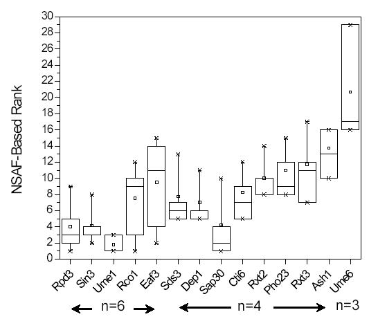
Specific proteins detected within a particular run were ranked based on their NSAF values calculated for each of the six analyses reported here (section 4.3, eq. 2). The distribution of these ranks for the 14 proteins belonging to Rpd3/Sin3 complexes was plotted as a box plot representation, where the 25^th and 75^th percentiles are represented by the upper and lower boundaries of the box, the median being the line dissecting the box, and the mean being the small square in each box. The 5^th and 95^th percentiles are shown with lines attached to the box, the ‘X’ represents the 1^st and 99^th percentiles, and the stand alone ‘–’ represents the complete range. The number (n) of runs in which each protein was detected is shown within arrows below the graph.

The normalization of spectral count can also be applied to proteins belonging to a specific complex to estimate the relative levels of each subunit within the complex [29, 30]. Here, for each of the 14 proteins h involved in the Rpd3L and/or Rpd3S complexes, we calculated a spectral abundance factor normalized against the complex (NcSAF) as follow:

$${(\text{NcSAF})}_h=\frac{{(\text{SpC/Length})}_h}{\sum _{j=1}^{14}{(\text{SpC/Length}h)}_j}$$ (eq. 3)

In the whole TAP preparations (Figure 4A), Rpd3, Sin3 and Ume1 had NcSAF values about twice the ones measured for the other proteins (with the exception of Sap30), most likely because these subunits were present in both Rpd3/Sin3 large and small complexes. While the MonoQ fractionation allowed to purify Rpd3/Sin3S away from the large complex (Figure 4C), the reverse was not true as small levels of the Rpd3/Sin3S specific subunits Eaf3 and Rco1 were detected in the large complex as well (Figure 4B). In the large complex, Rxt3, Ash1 and Ume6 were detected at substochiometric levels, indicating that they might not be present in all Rpd3/Sin3L complexes.

Figure 4. Spectral Abundance Factors Normalized against Subunits of Rpd3/Sin3 Complexes.

NcSAFs values for each of the 14 proteins belonging to Rpd3/Sin3 complexes were calculated (section 4.3, eq. 3) for whole TAP preparations (A), and large (B) and small (C) complex fractionations of Rpd3-TAP (black bars) and Sin3-TAP (gray bars) pull-downs.

References

- 1.Rigaut G, Shevchenko A, Rutz B, Wilm M, Mann M, Seraphin B. Nat Biotechnol. 1999;17:1030–1032. doi: 10.1038/13732. [DOI] [PubMed] [Google Scholar]
- 2.Gavin AC, Bosche M, Krause R, Grandi P, Marzioch M, Bauer A, Schultz J, Rick JM, Michon AM, Crucial CM, Remor M, Hofert C, Schelder M, Brajenovic M, Ruffner H, Merino A, Klein K, Hudak M, Dickson D, Rudi T, Gnau V, Bauch A, Bastuck S, Huhse B, Leutwein C, Heurtier MA, Copley RR, Edelmann A, Querfurth E, Rybin V, Drewes G, Raida M, Bouwmeester T, Bork P, Seraphin B, Kuster B, Neubauer G, Superti-Furga G. Nature. 2002;415:141–147. doi: 10.1038/415141a. [DOI] [PubMed] [Google Scholar]
- 3.Ho Y, Gruhler A, Heilbut A, Bader GD, Moore L, Adams SL, Millar A, Taylor P, Bennett K, Boutilier K, Yang L, Wolting C, Donaldson L, Schandorff S, Shewnarane J, Vo M, Taggart J, Goudreault M, Muskat B, Alfarano C, Dewar D, Lin Z, Michalickova K, Willems AR, Sassi H, Nielsen PA, Rasmussen KJ, Andersen JR, Johansen LE, Hansen LH, Jespersen H, Podtelejnikov A, Nielsen E, Crawford J, Poulsen V, Sorensen BD, Matthiesen J, Hendrickson RC, Gleeson F, Pawson T, Moran MF, Durocher D, Mann M, Hogue CW, Figeys D, Tyers M. Nature. 2002;415:180–183. doi: 10.1038/415180a. [DOI] [PubMed] [Google Scholar]
- 4.Einhauer A, Jungbauer A. J Chromatogr A. 2001;921:25–30. doi: 10.1016/s0021-9673(01)00831-7. [DOI] [PubMed] [Google Scholar]
- 5.von Mering C, Krause R, Snel B, Cornell M, Oliver SG, Fields S, Bork P. Nature. 2002;417:399–403. doi: 10.1038/nature750. [DOI] [PubMed] [Google Scholar]
- 6.Florens L, Washburn MP, Raine JD, Anthony RM, Grainger M, Haynes JD, Moch JK, Muster N, Sacci JB, Tabb DL, Witney AA, Wolters D, Wu Y, Gardner MJ, Holder AA, Sinden RE, Yates JR, Carucci DJ. Nature. 2002;419:520–526. doi: 10.1038/nature01107. [DOI] [PubMed] [Google Scholar]
- 7.Washburn MP, Wolters D, Yates JR., 3rd Nat Biotechnol. 2001;19:242–247. doi: 10.1038/85686. [DOI] [PubMed] [Google Scholar]
- 8.Graumann J, Dunipace LA, Seol JH, McDonald WH, Yates JR, 3rd, Wold BJ, Deshaies RJ. Mol Cell Proteomics. 2004;3:226–237. doi: 10.1074/mcp.M300099-MCP200. [DOI] [PubMed] [Google Scholar]
- 9.Sato S, Tomomori-Sato C, Parmery TJ, Florens L, Zybailov B, Swanson SK, Banks CA, Jin J, Cai Y, Washburn MP, Conaway JW, Conaway RC. Mol Cell. 2004;14:685–691. doi: 10.1016/j.molcel.2004.05.006. [DOI] [PubMed] [Google Scholar]
- 10.Carrozza MJ, Li B, Florens L, Suganuma T, Swanson SK, Lee KK, Shia WJ, Anderson S, Yates J, Washburn MP, Workman JL. Cell. 2005;123:581–592. doi: 10.1016/j.cell.2005.10.023. [DOI] [PubMed] [Google Scholar]
- 11.Eng J, McCormack AL, Yates JRI. J Am Soc Mass Spectrom. 1994;5:976–989. doi: 10.1016/1044-0305(94)80016-2. [DOI] [PubMed] [Google Scholar]
- 12.Tabb DL, McDonald WH, Yates JR., 3rd J Proteome Res. 2002;1:21–26. doi: 10.1021/pr015504q. [DOI] [PMC free article] [PubMed] [Google Scholar]
- 13.Liu H, Sadygov RG, Yates JR., 3rd Anal Chem. 2004;76:4193–4201. doi: 10.1021/ac0498563. [DOI] [PubMed] [Google Scholar]
- 14.Allet N, Barrillat N, Baussant T, Boiteau C, Botti P, Bougueleret L, Budin N, Canet D, Carraud S, Chiappe D, Christmann N, Colinge J, Cusin I, Dafflon N, Depresle B, Fasso I, Frauchiger P, Gaertner H, Gleizes A, Gonzalez-Couto E, Jeandenans C, Karmime A, Kowall T, Lagache S, Mahe E, Masselot A, Mattou H, Moniatte M, Niknejad A, Paolini M, Perret F, Pinaud N, Ranno F, Raimondi S, Reffas S, Regamey PO, Rey PA, Rodriguez-Tome P, Rose K, Rossellat G, Saudrais C, Schmidt C, Villain M, Zwahlen C. Proteomics. 2004;4:2333–2351. doi: 10.1002/pmic.200300840. [DOI] [PubMed] [Google Scholar]
- 15.Powell DW, Weaver CM, Jennings JL, McAfee KJ, He Y, Weil PA, Link AJ. Mol Cell Biol. 2004;24:7249–7259. doi: 10.1128/MCB.24.16.7249-7259.2004. [DOI] [PMC free article] [PubMed] [Google Scholar]
- 16.Gao J, Friedrichs MS, Dongre AR, Opiteck GJ. J Am Soc Mass Spectrom. 2005;16:1231–1238. doi: 10.1016/j.jasms.2004.12.002. [DOI] [PubMed] [Google Scholar]
- 17.Colinge J, Chiappe D, Lagache S, Moniatte M, Bougueleret L. Anal Chem. 2005;77:596–606. doi: 10.1021/ac0488513. [DOI] [PubMed] [Google Scholar]
- 18.Ishihama Y, Oda Y, Tabata T, Sato T, Nagasu T, Rappsilber J, Mann M. Mol Cell Proteomics. 2005;4:1265–1272. doi: 10.1074/mcp.M500061-MCP200. [DOI] [PubMed] [Google Scholar]
- 19.Old WM, Meyer-Arendt K, Aveline-Wolf L, Pierce KG, Mendoza A, Sevinsky JR, Resing KA, Ahn NG. Mol Cell Proteomics. 2005;4:1487–1502. doi: 10.1074/mcp.M500084-MCP200. [DOI] [PubMed] [Google Scholar]
- 20.Zybailov B, Coleman MK, Florens L, Washburn MP. Anal Chem. 2005;77:6218–6224. doi: 10.1021/ac050846r. [DOI] [PubMed] [Google Scholar]
- 21.Zybailov BL, Mosley AL, Sardiu ME, Coleman MK, Florens L, Washburn MP. J Proteome Res. 2006 doi: 10.1021/pr060161n. in press. [DOI] [PubMed] [Google Scholar]
- 22.Carrozza MJ, Florens L, Swanson SK, Shia WJ, Anderson S, Yates J, Washburn MP, Workman JL. Biochim Biophys Acta. 2005;1731:77–87. doi: 10.1016/j.bbaexp.2005.09.005. [DOI] [PubMed] [Google Scholar]
- 23.McDonald WH, Ohi R, Miyamoto DT, Mitchison TJ, Yates JR. Int J Mass Spectrom. 2002;219:245–251. [Google Scholar]
- 24.Florens L, Washburn MP. Methods Mol Biol. 2006;328:159–175. doi: 10.1385/1-59745-026-X:159. [DOI] [PubMed] [Google Scholar]
- 25.McDonald WH, Tabb DL, Sadygov RG, MacCoss MJ, Venable J, Graumann J, Johnson JR, Cociorva D, Yates JR., 3rd Rapid Commun Mass Spectrom. 2004;18:2162–2168. doi: 10.1002/rcm.1603. [DOI] [PubMed] [Google Scholar]
- 26.Sadygov RG, Eng J, Durr E, Saraf A, McDonald H, MacCoss MJ, Yates JR., 3rd J Proteome Res. 2002;1:211–215. doi: 10.1021/pr015514r. [DOI] [PubMed] [Google Scholar]
- 27.Xie H, Griffin TJ. J Proteome Res. 2006;5:1003–1009. doi: 10.1021/pr050472i. [DOI] [PubMed] [Google Scholar]
- 28.Peng J, Elias JE, Thoreen CC, Licklider LJ, Gygi SP. J Proteome Res. 2003;2:43–50. doi: 10.1021/pr025556v. [DOI] [PubMed] [Google Scholar]
- 29.Prochasson P, Florens L, Swanson SK, Washburn MP, Workman JL. Genes Dev. 2005;19:2534–2539. doi: 10.1101/gad.1341105. [DOI] [PMC free article] [PubMed] [Google Scholar]
- 30.Schneider J, Wood A, Lee JS, Schuster R, Dueker J, Maguire C, Swanson SK, Florens L, Washburn MP, Shilatifard A. Mol Cell. 2005;19:849–856. doi: 10.1016/j.molcel.2005.07.024. [DOI] [PubMed] [Google Scholar]