Item Response Theory and Health Outcomes Measurement in the 21st Century

Abstract

Item response theory (IRT) has a number of potential advantages over classical test theory in assessing self-reported health outcomes. IRT models yield invariant item and latent trait estimates (within a linear transformation), standard errors conditional on trait level, and trait estimates anchored to item content. IRT also facilitates evaluation of differential item functioning, inclusion of items with different response formats in the same scale, and assessment of person fit and is ideally suited for implementing computer adaptive testing. Finally, IRT methods can be helpful in developing better health outcome measures and in assessing change over time. These issues are reviewed, along with a discussion of some of the methodological and practical challenges in applying IRT methods.

Classical test theory (CTT) partitions observed item and scale responses into true score plus error. The person to whom the item is administered and the nature of the item itself influence the probability of a particular item response. A major limitation of CTT is that person ability and item difficulty cannot be estimated separately. In addition, CTT yields only a single reliability estimate and corresponding standard error of measurement, but the precision of measurement is known to vary by ability level.

Item response theory (IRT) comprises a set of generalized linear models and associated statistical procedures that connect observed survey responses to an examinee’s or a subject’s location on an unmeasured underlying (“latent”) trait.¹ IRT models have a number of potential advantages over CTT methods in assessing self-reported health outcomes. IRT models yield item and latent trait estimates (within a linear transformation) that do not vary with the characteristics of the population with respect to the underlying trait, standard errors conditional on trait level, and trait estimates linked to item content. In addition, IRT facilitates evaluation of whether items are equivalent in meaning to different respondents (differential item functioning) and inclusion of items with different response formats in the same scale, assessing person fit, and it is ideally suited for implementing computerized adaptive testing. IRT methods can also be helpful in developing better health outcome measures over time. After a basic introduction to IRT models, each of these issues is discussed. Then we discuss how IRT models can be useful in assessing change. Finally, we note some of the methodological and practical problems in applying IRT methods.

To illustrate results from real data, we refer to the 9-item measure of physical functioning administered to participants in the HIV Cost and Services Utilization Study (HCSUS).^2–4 Study participants were asked to indicate whether their health limited them a lot, a little, or not at all in each of the 9 activities during the past 4 weeks (see Appendix). The items were selected to represent a range of functioning, including basic activities of daily living (feeding oneself, bathing or dressing, preparing meals, or doing laundry), instrumental activities of daily living (shopping), mobility (getting around inside the home, climbing stairs, walking 1 block, walking >1 mile), and vigorous activities. Five items (vigorous activities, climbing 1 flight of stairs, walking >1 mile, walking 1 block, bathing or dressing) are identical to those in the SF-36 health survey.⁵

Item means, standard deviations, and the percentage not limited in each activity are provided in Table 1. The 9 items are scored on the 3-point response scale, with 1 representing limited a lot, 2 representing limited a little, and 3 representing not limited at all. Items are ordered by their means, which range from 1.97 (vigorous activities) to 2.90 (feeding yourself). These data will be used to provide an example of estimating item difficulty and discrimination parameters, category thresholds, model fit, and the unidimensionality assumption of IRT.

Table 1.

Item Means, Standard Deviations, and Percent Not Limited for 9 Physical Functioning Items

Item	Mean (SD)	Not Limited, %
Vigorous activities	1.97 (0.86)	45
Walking >1 mile	2.22 (0.84)	49
Climbing 1 flight of stairs	2.37 (0.76)	55
Shopping	2.61 (0.68)	72
Walking 1 block	2.63 (0.64)	72
Preparing meals or doing laundry	2.67 (0.63)	75
Bathing or dressing	2.80 (0.49)	84
Getting around inside your home	2.81 (0.47)	84
Feeding yourself	2.90 (0.36)	91

Items are scored 1 = yes, limited a lot; 2 = yes, limited a little; and 3 = no, not limited at all.

IRT Basics

IRT models are mathematical equations describing the association between a respondent’s underlying level on a latent trait and the probability of a particular item response using a nonlinear monotonic function.⁶ The correspondence between the predicted responses to an item and the latent trait is known as the item-characteristic curve (ICC). Most applications of IRT assume unidimensionality, and all IRT models assume local independence.⁷ Unidimensionality means that only 1 construct is measured by the items in a scale. Local independence means that the items are uncorrelated with each other when the latent trait or traits have been controlled for.⁸ In other words, local independence is obtained when the complete latent trait space is specified in the model. If the assumption of unidimensionality holds, then only a single latent trait is influencing item responses and local independence is obtained.

Item-Characteristic Curves

With dichotomous items, there tends to be an s-shaped relationship between increasing respondent trait level and increasing probability of endorsing an item. As shown in Figure 1, the ICC displays the nonlinear regression of the probability of a particular response (y axis) as a function of trait level (x axis). Items that produce a nonmonotonic association between trait level and response probability are unusual, but nonparametric IRT models have been developed.⁹ The middle of the ICC is steeper in slope, implying large changes in probability of an endorsement with small changes in trait level. Item discrimination corresponds to the slope of the ICC. The ICC for items with a higher probability of endorsement (easier items) are located farther to the left on the trait scale, and those with a lower probability of endorsement (harder items) are located further to the right (Figure 1). For example, Figure 1 shows ICCs for 3 items, each having 2 possible responses (dichotomous): (1) no and (2) yes. Item 1 is the “easiest” item because the probability of a “yes” response for a given trait level tends to be higher for it than for the other 2 items. Item 3 is the “hardest”item because the probability of a “yes” response for a given trait level tends to be lower than for the other 2 items.

Fig. 1.

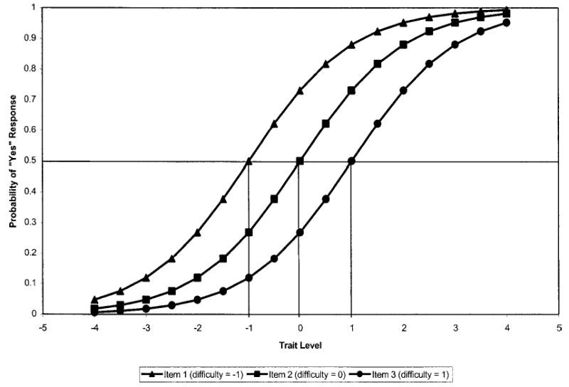
Item characteristic curves for 3 dichotomous items.

Dichotomous IRT Models

The different kinds of IRT models are distinguished by the functional form specified for the relationship between underlying ability and item response probability (ie, the ICC). For simplicity, we focus on dichotomous item models here and briefly describe examples for polytomous items (items with multiple response categories). Polytomous models are extensions of dichotomous IRT models. The features of the 3 main types of dichotomous IRT models are summarized in Table 2. As noted, each of these models estimates an item difficulty parameter. The 2- and 3-parameter models also estimate an item discrimination parameter. Finally, the 3-parameter model includes a “guessing” parameter.

Table 2.

Features of Different Types of Dichotomous IRT Models

	Item Difficulty	Item Discrimination	Guessing Parameter
1-Parameter (Rasch)	X
2-Parameter	X	X
3-Parameter	X	X	X

This article takes the position that the Rasch model is nested within the 2- and 3-parameter models. We do not address the side debate in the literature about whether the Rasch model should be referred to as distinct rather than a special case of IRT models.

One-Parameter Model

The Rasch model specifies a 1-parameter logistic (1-PL) function.^10,11 The 1-PL model allows items to vary in their difficulty level (probability of endorsement or scoring high on the item), but it assumes that all items are equally discriminating (the item discrimination parameter, α, is fixed at the same value for all items). Observed dichotomous item responses are a function of the latent trait (θ) and the difficulty of the item (β):

$$\text{P}({\theta }_{\text{I}})={\text{e}}^{\text{D}\alpha (\theta -\beta )}/[1+{\text{e}}^{\text{D}\alpha (\theta -\beta )}]=1/[1+{\text{e}}^{-\text{D}\alpha (\theta -\beta )}]$$

D is a scaling factor that can be used to make the logistic function essentially the same as the normal ogive model (ie, setting D = 1.7). Latent trait scores and item difficulty parameters are estimated independently, and both values are on the same z-score metric (constrained to sum to zero). Most trait scores and difficulty estimates fall between −2 and 2.

The difficulty parameter indicates the ability level or trait level needed to have a 50% chance of endorsing an item (eg, responding “yes”to a “yes or no”item). In the Rasch model, the log odds of a person endorsing or responding in the higher category is simply the difference between trait level and the item difficulty. A nice feature of the Rasch model is that observed raw scores are sufficient for estimating latent trait scores using a nonlinear transformation. In other IRT models, the raw score is not a sufficient statistic.

Figure 1 presents ICCs for 3 dichotomous items, differing in their degree of difficulty on the z-score metric from −1, 0, to 1. Note that the s-shaped curves are parallel (have the same slope) because only item difficulty is allowed to vary in the 1-PL model. The probability of a “yes” response to the easiest item (β₁ = −1) for someone of average ability (θ = 0) is ~0.73, whereas the probability for the item with the intermediate difficulty level (β₂ = 0) is 0.50 (this is true by definition given its difficulty level), and the probability for the hardest items (β₃ = 1) is 0.27. The discrimination parameter of each item was set to 1.0.

For purposes of illustration of the Rasch model, we dichotomized the items by collapsing the “yes, limited a lot”and the “yes, limited a little”response options together and coding this 0. The “no, not limited”at all response was coded 1. We fit a 1-PL model to these data using MULTILOG¹² (see Table 3). Slope (discrimination) estimates are typically fixed at 1.0 in the absence of any information. In this example, the slopes were fixed at 3.49 by MULTILOG on the basis of the generally high level of discrimination for this set of items.

Table 3.

Item Difficulty Estimates for Physical Functioning Items: Rasch Model

Item	Item Difficulty (SE)
Vigorous activities	0.46 (0.02)
Walking >1 mile	0.06 (0.03)
Climbing 1 flight of stairs	−0.14 (0.02)
Shopping	−0.65 (0.02)
Walking 1 block	−0.67 (0.02)
Preparing meals or doing laundry	−0.78 (0.03)
Bathing or dressing	−1.18 (0.03)
Getting around inside your home	−1.19 (0.03)
Feeding yourself	−1.60 (0.04)

Items are ordered by difficulty level. Estimates were obtained from MULTILOG, version 6.30. Slopes were fixed at 3.49.

Item difficulty estimates (Table 3) ranged from −1.60 (feeding yourself) to 0.46 (vigorous activities). The second hardest item was walking >1 mile, followed by climbing 1 flight of stairs, shopping, walking 1 block, bathing or dressing, and getting around inside the home.

Two-Parameter Model

The 2-parameter (2-PL) IRT model extends the 1-PL Rasch model by estimating an item discrimination parameter (α) and an item difficulty parameter. The discrimination parameter is similar to an item-total correlation and typically ranges from ~0.5 to 2. Higher values of this parameter are associated with items that are better able to discriminate between contiguous trait levels near the inflection point. This is manifested as a steeper slope in the graph of the probability of a particular response (y axis) by underlying ability or trait level (x axis). An important feature of the 2-PL model is that the distance between an individual’s trait level and item difficulty has a greater effect on the probability of endorsing highly discriminating items than on less discriminating items. Thus, more discriminating items provide greater information about a respondent than do less discriminating items. Unlike the Rasch model, discrimination needs to be incorporated, and the raw score is not sufficient for estimating trait scores.

We also fit a 2-PL model for the dichotomized physical functioning items (Table 4). Difficulty estimates were similar to those reported above for the 1-PL model, ranging from −1.62 (feeding yourself) to 0.49 (vigorous activities). Thus, difficulty estimates were robust to whether or not the item discrimination parameter was estimated. Item discriminations (slopes) ranged from 2.51 (vigorous activities) to 4.09 (walking >1 mile). These slopes are very high; each one exceeds the upper value (2.00) of the typical range noted above.

Table 4.

Item Difficulty and Discrimination Estimates for Physical Functioning Items: Two-Parameter Model

Item	Item Difficulty (SE)	Discrimination (SE)
Vigorous activities	0.49 (0.03)	2.51 (0.12)
Walking >1 mile	0.06 (0.02)	4.09 (0.19)
Climbing 1 flight of stairs	−0.14 (0.03)	3.46 (0.15)
Shopping	−0.64 (0.02)	3.74 (0.26)
Walking 1 block	−0.66 (0.02)	3.69 (0.26)
Preparing meals or doing laundry	−0.76 (0.03)	3.83 (0.25)
Bathing or dressing	−1.18 (0.03)	3.52 (0.21)
Getting around inside your home	−1.18 (0.03)	3.59 (0.21)
Feeding yourself	−1.62 (0.05)	3.21 (0.25)

Items are ordered by difficulty level. Estimates were obtained from MULTILOG, version 6.30.

Three-Parameter Model

The 3-parameter (3-PL) model includes a pseudo-guessing parameter (c), as well as item discrimination and difficulty parameters: P(θ_I) = c + (1−c)e^Dα(θ−β)/(1 +e^Dα(θ−β)). This additional parameter adjusts for the impact of chance on observed scores. In the 3-PL model, the probability of the response at θ = β = (1 + c)/2. In ability testing, examinees can get an answer right by chance, raising the lower asymptote of the function. The relevance of this parameter to HRQOL assessment remains to be demonstrated. Response error, rather than guessing, is a plausible third parameter for health outcomes measurement.

Examples of Polytomous IRT Models

Graded Response Model

The graded response model,¹³ an extension of the 2-PL logistic model, is appropriate to use when item responses can be characterized as ordered categorical responses. In the graded response model, each item is described by a slope parameter and between category threshold parameters (one less than the number of response categories). For the graded response model, 1 operating characteristic curve needs to be estimated for each between category threshold. In the graded response model, items need not have the same number of response categories. Threshold parameters represent the trait level necessary to respond above threshold with 0.50 probability. Category response curves represent the probability of responding in a particular category conditional on trait level. Generally speaking, items with higher slope parameters provide more item information. The spread of the item information and where on the trait continuum information is peaked are determined by the between-category threshold parameters.

We fit the graded response model to the HCSUS physical functioning items, preserving the original 3-point response scale. Responses were scored as shown in the Appendix: 1 = yes, limited a lot; 2= yes, limited a little; and 3 = no, not limited at all. In running the model, 2 category threshold parameters and 1 slope parameter were estimated for each item.

Table 5 shows the category threshold parameters and the slope parameter for each of the 9 physical functioning items. The category threshold parameters represent the point along the latent trait scale at which a respondent has a 0.50 probability of responding above the threshold. Looking at the first row of Table 5, one can see that a person with a trait level of 0.62 has a 50/50 chance of responding “not limited at all”in vigorous activities. Similarly, a person with a trait level of −0.31 has a 50/50 chance of responding “limited a little” or “not limited at all” in vigorous activities. The trait level associated with a 0.50 probability of responding above the 2 thresholds is higher for the vigorous activities item than for any of the other 8 physical functioning items. This is consistent with the fact that more people reported limitations in vigorous activities than on any of the other items. For example, 65% of the sample reported being limited in vigorous activities compared with only 9% for feeding.

Table 5.

Category Thresholds and Slope Estimates for HCSUS Physical Functioning Items: Graded Response Model

Item	Category Threshold Parameter—Between “A Lot” and “A Little” (SE)	Category Threshold Parameter—Between “A Little” and “Not at All” (SE)	Slope Parameter (SE)
Vigorous activities	−0.31 (0.03)	0.62 (0.04)	2.22 (0.09)
Climbing 1 flight of stairs	−1.09 (0.04)	−0.05 (0.03)	2.77 (0.10)
Walking >1 mile	−0.65 (0.03)	0.17 (0.03)	3.28 (0.13)
Walking 1 block	−1.56 (0.04)	−0.62 (0.03)	3.27 (0.19)
Bathing or dressing	−2.03 (0.07)	−1.13 (0.03)	3.25 (0.20)
Preparing meals or doing laundry	−1.59 (0.04)	−0.73 (0.03)	3.27 (0.19)
Shopping	−1.41 (0.04)	−0.59 (0.03)	3.39 (0.16)
Getting around inside your home	−2.14 (0.07)	−1.14 (0.04)	3.18 (0.18)
Feeding yourself	−2.73 (0.12)	−1.71 (0.06)	2.35 (0.18)

Estimates were obtained from MULTILOG, version 6.30.

Partial Credit Model

The partial credit model¹⁴ is an extension of the Rasch model to polytomous items. Thus, item slopes are assumed to be equal across items. The model depicts the probability of a person responding in category x as a function of the difference between their trait level and a category intersection parameter. These intersection parameters represent the trait level at which a response in a category becomes more likely than a response in the previous category. The number of category intersection parameters is equal to one less than the number of response options. The partial credit model makes no assumption about rank ordering of response categories on the underlying continuum.

Rating Scale Model

The rating scale model¹⁵ assumes that the response categories are ordered. Response categories are assigned intersection parameters that are considered equal across items, and item location is described by a single scale location parameter. The location parameter represents the average difficulty for a particular item relative to the category intersections. Each item is assumed to provide the same amount of information and have the same slope. Therefore, the rating scale model is also an extension of the Rasch model.

Assessing Model Fit

Choosing which model to use depends on the reasonableness of the assumptions about the scale items in the particular application.¹⁶ Unlike CTT, the reasonableness of the IRT model can be evaluated by examining its fit to the data. Dimensionality should be evaluated before choosing an IRT model. Tests of equal discrimination should be conducted before choosing a 1-PL model, and tests of minimal guessing, if relevant, should be conducted before choosing a 2-PL model. Finally, item fit χ² statistics¹⁷ and model residuals can be examined as a means of checking model predictions against actual test data (Table 6). The mean discrepancy (absolute values) across the 9 items and 3 response categories was 0.1 (SD = 0.01). The item fit χ² statistics were significant (P < 0.05) for all items. Because statistical power increases with sample size, larger samples lead to a greater likelihood of significant χ² differences. Appropriate caution is needed in interpreting χ² statistics. The results in Table 6 suggest minimal practical differences between observed and expected response frequencies.

Table 6.

Difference Between Observed and Expected Response Frequencies (Absolute Values) by Item and Response Category

	Yes, Limited a Lot	Yes, Limited a Little	No, Not Limited at All	P
Vigorous activities	0.01	0.02	0.02	<0.05
Walking >1 mile	0.01	0.02	0.02	<0.05
Climbing 1 flight of stairs	0.01	0.03	0.03	<0.05
Shopping	0.01	0.01	0.01	<0.05
Walking 1 block	0.01	0.01	0.01	<0.05
Preparing meals or doing laundry	0.01	0.00	0.01	<0.05
Bathing or dressing	0.01	0.01	0.00	<0.05
Getting around inside your home	0.00	0.00	0.02	<0.05
Feeding yourself	0.01	0.01	0.01	<0.05

The mean difference (absolute values) between the observed and expected response frequencies across all items and all response categories was 0.01 (SD = 0.01). The reported P values are based on the item-fit χ² reported by Parscale 3.5.

Potential Advantages of Using IRT in Assessing Health Outcome Assessment

Table 7 lists some of the advantages of using IRT in health outcome assessment. This section summarizes these potential advantages.

Table 7.

Potential Advantages of Using IRT in Health Outcomes Assessment

More comprehensive and accurate evaluation of item characteristics Assess group differences in item and scale functioning Evaluate scales containing items with different response formats Improve existing measures CAT Model change Evaluate person fit

More Comprehensive and Accurate Evaluation of Item Characteristics

Invariant Item and Latent Trait Estimates

In CTT, item means are confounded by valid group differences, and item-scale correlations are affected by group variability on the construct. When an IRT model fits the data exactly in the population, sample invariant item and latent trait estimates are possible.^18,19 Within sampling error, the ICC should be the same regardless of what sample it was derived from (within a linear transformation), and the person estimates should be the same regardless of what items they are based on.

Invariance is a population property that cannot be directly observed but can be evaluated within a sample. For instance, one can look to see if individual scores are the same regardless of what items are administered or whether item parameters are the same across subsets of the sample. Embretson²⁰ illustrated with simulations that CTT estimates of item difficulty for different subgroups of the population can vary considerably and the association between the estimates can be nonlinear. In contrast, difficulty estimates derived from the Rasch model were robust and very highly correlated (r = 0.997).

Item and Scale Information Conditional on Trait Level

Any ICC can be transformed into an item information curve (utility of information curves is dependent on how well the ICC fits the data).¹⁹ Information curves are analogous to reliability of measurement and indicate the precision (reciprocal of the error variance) of an item or test along the underlying trait continuum. An item provides the most information around its difficulty level. The maximum information lies at β in the 1-PL and 2-PL models. In a 3-PL model, the maximum information is not quite at β because as c decreases information increases (all else being equal). The steeper the slope in the ICC and the smaller the item variance, the greater the item information.

Scale information depends on the number of items and how good the items are. The information provided by a multi-item scale is simply the sum of the item information functions. Standard error of measurement in IRT models is inversely related to information and hence is conditional on trait level: SE = 1/(information|θ)^1/2. Because information varies by trait level, a scale may be quite precise for some people and not so precise for others. It is also possible to average the individual standard errors to obtain a composite estimate for the population.²⁰ This means that items can be selected that are most informative for specific subgroups of the population.

To illustrate the information function, the formula for the 3-PL logistic model is given below:

$$I({\theta }_{\text{I}})=2.89{\alpha }_{\text{i}}^2(1-{\text{c}}_{\text{i}})/[{\text{c}}_{\text{I}}+{\text{e}}^{1.7\alpha (\theta -\beta \text{i})}]\times {[1+e^{-1.7\alpha (\theta -\beta \text{i})}]}^2$$

Working through this equation shows that information is higher when the difficulty of the item is closer to the trait level, when the discrimination parameter is higher, and when the pseudo-guessing parameter, c, is smaller. Figure 2 plots item information curves for 3 items that vary in the 3-PL parameters: item 1 (c = 0.0; β = −1.5; α = 1.8), item 2 (c = 0.1; β = −0.5; α = 1.2), and item 3 (c = 0.0; β = 1.0; α= 1.8). Note that the information peaks at the difficulty level for items 1 and 3, because c = 0.0 for both of these items. For item 2, information peaks close to its difficulty level, but the peak is shifted a little because of the 0.1 c parameter.

Fig. 2.

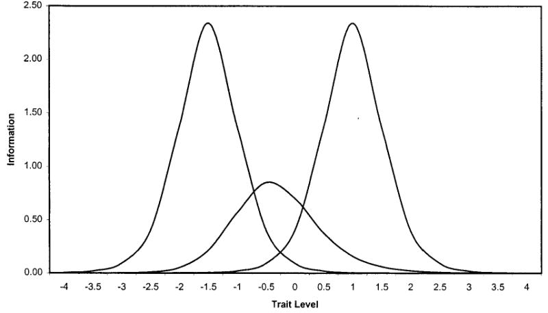
Item information functions for 3 polytomous items: 3-PL model.

Trait Estimates Anchored to Item Content

In CTT, the scale score is not typically informative about the item response pattern. However, if dichotomous items are consistent with a Guttman scale,²¹ then they are ordered along a single dimension in terms of their difficulty, and the pattern of responses to items is determined by the sum of the endorsed items. The linkage between trait level and item content in IRT is similar to the Guttman scale, but IRT models are probabilistic rather than deterministic.

In IRT, item and trait parameters are on the same metric, and the meaning of trait scores can be related directly to the probability of item responses. Hence, it is possible to obtain a relatively concrete picture of response pattern probabilities for an individual given the trait score. If the person’s trait level exceeds the difficulty of an item, then the person is more likely than not to “pass” or endorse this item. Conversely, if the trait level is below the item difficulty, then the person is less likely to endorse than not endorse the item.

Assessing Group Differences in Item and Scale Functioning

IRT methods provide an ideal basis for assessing differential item functioning (DIF), defined as different probabilities of endorsing an item by respondents from 2 groups who are equal on the latent trait. When DIF is present, scoring respondents on the latent trait using a common set of item parameters causes trait estimates to be too high or too low for those in 1 group relative to the other.^22,23 DIF is identified by looking to see if item characteristic curves differ (item parameters differ) by group.²⁴

One way to assess DIF is to fit multigroup IRT models in which the slope and difficulty parameters are freely estimated versus constrained to be equal for different groups. If the less constrained model fits the data better, this suggests that there is significant DIF. For example, Morales et al²⁵ compared satisfaction with care responses between whites and Hispanics in a study of patients receiving medical care from an association of 48 physician groups.²⁶ This analysis revealed that 2 of 9 items functioned differently in the 2 groups but that the DIF did not have meaningful impact on trait scores. When all 9 items were included in the satisfaction scale, the effect size was 0.27, with whites rating care significantly more positively than Hispanics. When the biased items were dropped from the scale, the effect size became 0.26 and the mean scale scores remained significantly different. Thus, statistically significant DIF does not necessarily invalidate comparisons between groups.

Evaluating Scales Containing Items With Different Response Formats

In CTT, typically one tries to avoid combining items with different variances because they have differential impact on raw scale scores. It is possible in CTT to convert items with different response options to a common range of scores (eg, 0 to 100) or to standardize the items so that they have the same mean and standard deviation before combining them. However, these procedures yield arbitrary weighting of items toward the scale score. IRT requires only that item responses have a specifiable relationship with the underlying construct.²⁷ IRT models, such as the graded response model, have been developed that allow different items to have varying numbers of response categories.¹³

Improving Existing Measures

One possible benefit of IRT is facilitation of the development of new items to improve existing measures. Because standard errors of measurement are estimated conditional on trait level, IRT methods provide a strong basis for identifying where along the trait continuum the measurement provides little information and is in need of improvement. The ideal measure will provide high information at the locations of the trait continuum that are important for the intended application. For example, it may be necessary to identify only people who score so high on a depression scale that mental health counseling is needed to prevent a psychological crisis from occurring. The desired information function would be one that is highly peaked at the trait level associated with the depressive symptom threshold.

IRT statistics cannot tell the researcher how to write better items or exactly what items will fill an identified gap in the item difficulty range. Poorly fitting items can provide a clue to the types of things to avoid when writing new items. An item with a double negative may not fit very well because of respondent confusion. Items bounding the target difficulty range can provide anchors for items that need to be written.

For example, a Rasch analysis of the SF-36 physical functioning scale resulted in log-odds (logits) item location estimates of −1.93 for walking 1 block compared with −3.44 for bathing or dressing.²⁸ To fill the gap between these difficulty levels, one might decide to write an item about preparing meals or laundry. This could be based on intuition about where the item will land or on existing data including CTT estimates of item difficulty.

Computerized Adaptive Testing

CTT scales tend to be long because they are designed to produce a high coefficient α.^29,30 But most of the items are a waste of time for any particular respondent because they yield little information. In contrast, IRT methods make it possible to estimate person trait levels with any subset of items in an item pool. Computerized adaptive testing (CAT) is ideally suited to IRT. Traditional, fixed-length tests require administering items that are high for those with low trait values and items that are too low for those with high trait values.

There are multiple CAT algorithms.³¹ We describe one example here to illustrate the general approach. First, an item bank of highly discriminating items of varying difficulty levels is developed. Then each item administered is targeted at the trait level of the respondent. Without any prior information, the first item administered is often a randomly selected item of medium difficulty. After each response, examinee trait level and its standard error are estimated. If maximum likelihood is used to estimate trait level, step-size scoring (eg, 0.25 increment up or down) can be used after the first item is administered. The next item administered to those not endorsing the first item is an easier item located the specified step away from the first item. If the person endorses the item, the next item administered is a harder item located the specified step away. After 1 item has been endorsed and 1 not endorsed, maximum likelihood scoring is possible and begun. The next item selected is an item that maximizes the likelihood function (ie, item with a 50% chance of endorsement in the 1- and 2-PL models). CAT is terminated when the standard error falls below an acceptable value. Note that CAT algorithms can be designed for polytomous items as well.

Modeling Change

IRT models are well suited for tracking change in health. IRT models offer considerable flexibility in longitudinal studies when the same items have not been administered at every data collection wave. Because trait level can be estimated from any subset of items, it is possible to have a good trait estimate even if the items are not identical at different time points. Thus, the optimal subset of items could be administered in theory to different respondents, and this optimal subset would vary, depending on their trait level at each time point. This feature of IRT models means that respondent burden is minimized. Each respondent can be administered only the number of items that are needed to establish a satisfactory small enough standard error of measurement. This feature of IRT also will help to ensure that the reliability of measurement is sufficiently high to allow for monitoring individual patients over time.

IRT can also help address the issue of clinically important difference or change (see the article by Testa et al³² in this issue). Anchor-based approaches have been proposed that compare prospectively measured change in health to change on a clinical parameter (eg, viral load) or to retrospectively reported global change.³³ For example, the change in a health-related quality of life scale associated with going from detectable to undetectable levels of viral load in people with HIV disease might be deemed clinically important. Because IRT trait estimates have direct implications for the probability of item responses and items are arrayed along a single continuum, substantive meaning can be attached to point-in-time and change scores. Trait level change can therefore be cast in light of concrete change in levels of functioning and well-being to help determine the threshold for clinically meaningful change.

One suggested advantage of IRT over CTT is interval level as opposed to ordinal level measurement. Although interval level and even ratio level measurement has been argued for Rasch models³⁴ and a nonlinear transformation of trait level estimates can provide ratio-scale type of interpretation,³⁵ the trait level scale is not strictly an interval scale. However, it has been noted that assessing change in terms of estimated trait level rather than raw scores can yield more accurate estimates of change.³⁶ Ongoing work directed at item response theory models of change for within-subject change that can be extended to group level change offers exciting possibilities for longitudinal analyses.³⁷

Evaluating Person Fit

An important development in the use of IRT methods is detection of the extent to which a person’s pattern of item responses is consistent with the IRT model.^38–40 Person fit indexes have been developed for this purpose. The standardized Z_L Fit Index is one such index: Z_L|θ_I = ∑[ln L|θ_I − ∑E(ln L|θ_I]/(∑V[ln L|θ_I)),1/2 where ln = natural logarithm. Large negative Z_L values (Z_L< = −2.0) indicate misfit. Large positive Z_L values indicate response patterns that are higher in likelihood than the model predicts.

Depending on the context, person misfit can be suggestive of an aberrant respondent, response carelessness, cognitive errors, fumbling, or cheating. The bottom line is that person misfit is a red flag that should be explored. For example, unpublished baseline data from HCSUS revealed a large negative Z_L index⁴¹ for a respondent who reported that he was “limited a lot” in feeding, getting around inside his home, preparing meals, shopping, and climbing 1 flight of stairs but only “limited a little” in vigorous activities, walking >1 mile, and walking 1 block. The apparent inconsistencies in this response pattern suggests the possibility of carelessness in answers given in this face-to-face interview.

Methodological and Practical Challenges in Applying IRT Methods

Unidimensionality

In evaluations of dimensionality in the context of exploratory factor analysis, it has been recommended that one examine multiple criteria such as the scree test,⁴² the Kaiser-Guttman eigen values >1.00 rule, the ratio of first to second eigenvalues, parallel analysis,⁴³ the Tucker-Lewis⁴⁴ reliability coefficient, residual analysis,⁴⁵ and interpretability of resulting factors.⁴⁶ Determining the extent to which items are unidimensional is important in IRT analysis because this is a fundamental assumption of the method. Multidimensional IRT models have been developed.⁷

It is generally acknowledged that the assumption of unidimensionality “cannot be strictly met because several cognitive, personality, and test-taking factors always affect test performance, at least to some extent.”¹⁹ As a result, there has been recognition that establishing “essential unidimensionality” is sufficient for satisfying this assumption. Stout^47,48 developed a procedure by which to judge whether or not a data set is essentially unidimensional. In short, a scale is essentially unidimensional when the average between-item residual covariances after fitting a 1-factor model approaches zero as the length of the scale increases.

Essential unidimensionality can be illustrated conceptually by use of a previously published example. In confirmatory factor analysis, it is possible that multiple factors provide a better fit to the data than a single dimension. Categorical confirmatory factor analytic models can now be estimated.^49,50 The estimated correlation between 2 factors can be fixed at 1.0, and the fit of this model can be contrasted to a model that allows the factor correlation to be estimated. A χ² test of the significance of the difference in model fit (1 df) can be used to determine whether 2 factors provide a better fit to the data. Even when 2 factors are extremely highly correlated (eg, r = 0.90), a 2-factor model might provide better fit to the data than a 1-factor model.⁵¹ Thus, statistical tests alone cannot be trusted to provide a reasonable answer about dimensionality. This is a case in which, even though unidimensionality was not fully satisfied, the items may be considered to have essential unidimensionality.

The 9 physical functioning items described earlier are polytomous (ie, have 3 response choices). We tested the unidimensionality assumption of IRT by fitting 1-factor categorical confirmatory factor analysis.⁴⁹ The model was statistically rejectable because of the large sample size (λ² = 1,059.29, n = 2,829, df = 27, P < 0.001), but it fit the data well according to practical fit indexes (comparative fit index = 0.99). Standardized factor loadings ranged from 0.72 to 0.94, and the average absolute standardized residual was 0.05.

When Does IRT Matter?

Independent of whether IRT scoring improves on classic approaches to estimating true scores, IRT is likely to be viewed as a better way of analyzing measures. Nonetheless, there is interest in the comparability of CTT and IRT-based item and person statistics. Recently, Fan⁵² used data collected from 11th graders on the Texas Assessment of Academic Skills to compare CTT and IRT parameter estimates. The academic skills assessment battery included a 48-item reading test and a 60-item math test, with each of the multiple choice items scored correct or incorrect. Twenty random samples of 1,000 examinees were drawn from a pool of more than 193,000 participants.

CTT item difficulty estimates were the proportion of examinees passing each item, transformed to a the (1−p)th percentile from the z distribution. This transformation assumed that the underlying trait measured by each item was normally distributed. CTT item discrimination estimates were obtained by taking the Fisher z transformation of the item-scale correlation: z = [ln(1 + r) − ln(1−r)]/2. Fan⁵² found that the CTT and IRT item difficulty and discrimination estimates were very similar. In this particular application, the resulting estimates did not change as a result of using the more sophisticated IRT methodology.

In theory, there are many possibilities for identifying meaningful differences between CTT and IRT. Because IRT models may better reflect actual response patterns, one would expect IRT estimates to be more accurate reflections of true status than CTT estimates. As a result, IRT estimates of health outcomes should be more sensitive to true cross-sectional differences and more responsive to change in health over time. Indeed, a recent study found that the sensitivity of the SF-36 physical functioning scale to differences in disease severity was greater for Rasch model–based scoring than for simple summated scoring.⁵³ Similarly, a study of 194 individuals with multiple sclerosis⁵⁴ revealed that the RAND-36 HIS mental health composite score, an IRT-based summary measure,⁵⁵ correlated more strongly with the Expanded Disability Status Scale than did the SF-36 mental health summary score, a CTT-based measure. Moreover, the RAND-36 scores were found to be more responsive to change in seizure frequency than the SF-36 scores in a sample of 142 adults participating in a randomized controlled trial of an antiepileptic drug.⁵⁶

Because nonlinear transformations of dependent variables can either eliminate or create interactions between independent variables, apparent interactions in raw scores may vanish (and vice versa) when scored with IRT.⁵⁷ Given the greater complexity and difficulty of IRT model–based estimates, it is important to document when IRT scoring (trait estimates) makes a difference.

Practical Problems in Applying IRT

There are a variety of software products available that can be used to analyze health outcomes data with IRT methods, including BIGSTEPS/WINSTEPS,⁵⁸ MULTILOG,¹² and PARSCALE.⁵⁹ BIGSTEPS implements the 1-PL model. MULTILOG can estimate dichotomous or polytomous 1-, 2- and 3-PL models; Samejima’s graded response model; Master’s partial credit model; and Bock’s nominal response model. Maximum likelihood and marginal maximum likelihood estimates can be obtained. PARSCALE estimates 1-, 2-, and 3-PL logistic models; Samejima’s graded response model; Muraki’s modification of the graded response model (rating scale version); the partial credit model; and the generalized partial credit model.

None of these programs are particularly easy to learn and implement. The documentation is often difficult to read, and finding out the reason for program failures can be time consuming and frustrating. The existing programs have a striking similarity to the early versions of the LISREL structural equation-modeling program.⁶⁰ LISREL required a translation of familiar equation language into matrixes and Greek letters. Widespread adoption of IRT in health outcome studies will be facilitated by the development of user-friendly software.

Conclusions

IRT methods will be used in health outcome measurement on a rapidly increasing basis in the 21st century. The growing experience among health services researchers will lead to enhancements of the method’s utility for the field and improvements in the collective applications of the methodology. We look forward to a productive 100 years of IRT and health outcomes measurement.

Fig. 3.

Physical functioning items in HCSUS. R indicates respondent.

References

- 1.Mellenbergh GJ. Generalized linear item response theory. Psychol Bull. 1994;15:300–307. [Google Scholar]
- 2.Hays RD, Spritzer KL, McCaffrey D, Cleary PD, Collins R, Sherbourne C, et al. The HIV Cost and Services Utilization Study (HCSUS) measures of health-related quality of life. Santa Monica, Calif: RAND; 1998. DRU-1897-AHCPR. [Google Scholar]
- 3.Shapiro MF, Morton SC, McCaffrey DF, Senterfitt JW, Fleishman JA, Perlman JF, et al. Variations in the care of HIV-infected adults in the United States: Results from the HIV Cost and Services Utilization Study. JAMA. 1999;281:2305–2315. doi: 10.1001/jama.281.24.2305. [DOI] [PubMed] [Google Scholar]
- 4.Wu AW, Hays RD, Kelly S, Malitz F, Bozzette SA. Applications of the Medical Outcomes Study health-related quality of life measures in HIV/AIDS. Qual Life Res. 1997;6:531–554. doi: 10.1023/a:1018460132567. [DOI] [PubMed] [Google Scholar]
- 5.Ware JE, Sherbourne CD. The MOS 36-item short-form health survey (SF-36), I: Conceptual framework and item selection. Med Care. 1992;30:473–483. [PubMed] [Google Scholar]
- 6.Reise SP, Widaman KF, Pugh RH. Confirmatory factor analysis and item response theory: Two approaches for exploring measurement invariance. Psychol Bull. 1993;114:552–566. doi: 10.1037/0033-2909.114.3.552. [DOI] [PubMed] [Google Scholar]
- 7.Reckase MD. The past and future of multidimensional item response theory. Appl Psychol Meas. 1997;21:25–36. [Google Scholar]
- 8.McDonald RP. The dimensionality of tests and items. Br J Math Stat Psychol. 1981;34:100–117. [Google Scholar]
- 9.Santor DA, Ramsay JO, Zuroff DC. Nonparametric item analyses of the Beck Depression Inventory: Evaluating gender item bias and response option weights. Psychol Assess. 1994;6:255–270. [Google Scholar]
- 10.Rasch G. An individualistic approach to item analysis. In: Lazarsfeld PF, Henry NW, editors. Readings in mathematical social science. Cambridge, Mass: Massachusetts Institute of Technology Press; 1966. pp. 89–108. [Google Scholar]
- 11.Rasch G. Probabilistic models for some intelligence and attainment tests. Copenhagen, Denmark: Danmarks Paedogogiske Institut; 1960. [Google Scholar]
- 12.Thissen D. MULTILOG user’s guide: Multiple categorical item analysis and test scoring using item response theory. Chicago, Ill: Scientific Software, Inc; 1991. [Google Scholar]
- 13.Samejima F. The graded response model. In: van der Linden WJ, Hambleton R, editors. Handbook of modern item response theory. New York, NY: Springer; 1996. pp. 85–100. [Google Scholar]
- 14.Masters GN. A Rasch model for partial credit scoring. Psychometrika. 1992;47:149–174. [Google Scholar]
- 15.Andrich D. A rating formulation for ordered response categories. Psychometrika. 1978;43:561–573. [Google Scholar]
- 16.Andrich D. Distinctive and incompatible properties of two common classes of IRT models for graded responses. Appl Psychol Meas. 1995;19:101–119. [Google Scholar]
- 17.McDonald RP, Mok MMC. Goodness of fit in item response models. Multivariate Behav Res. 1995;30:23–40. doi: 10.1207/s15327906mbr3001_2. [DOI] [PubMed] [Google Scholar]
- 18.Bejar II. A procedure for investigating the unidimensionality of achievement tests based on item parameter estimates. J Educ Meas. 1980;17:283–296. [Google Scholar]
- 19.Hambleton RK, Swaminathan H, Rogers HJ. Fundamentals of item response theory. Newbury Park, Calif: Sage; 1991. [Google Scholar]
- 20.Embretson SE. The new rules of measurement. Psychol Assess. 1996;8:341–349. [Google Scholar]
- 21.Menzel H. A new coefficient for scalogram analysis. Public Opinion Q. 1953;17:268–280. [Google Scholar]
- 22.Holland PW, Wainer H. Differential item functioning. Hillsdale, NJ: Erlbaum; 1993. [Google Scholar]
- 23.Milsap RE, Everson HT. Methodology review: Statistical approaches for assessing measurement bias. Appl Psychol Meas. 1993;17:297–334. [Google Scholar]
- 24.Reise SP, Widaman KF, Pugh RH. Confirmatory factor analysis and item response theory: Two approaches for exploring measurement invariance. Psychol Bull. 1993;114:552–566. doi: 10.1037/0033-2909.114.3.552. [DOI] [PubMed] [Google Scholar]
- 25.Morales LS, Reise SP, Hays RD. Evaluating the equivalence of health care ratings by whites and Hispanics. Med Care. 2000;38:517–527. doi: 10.1097/00005650-200005000-00008. [DOI] [PMC free article] [PubMed] [Google Scholar]
- 26.Hays RD, Brown JA, Spritzer KL, Dixon WJ, Brook RH. Satisfaction with health care provided by 48 physician groups. Arch Intern Med. 1998;158:785–790. doi: 10.1001/archinte.158.7.785. [DOI] [PubMed] [Google Scholar]
- 27.Thissen D. Repealing rules that no longer apply to psychological measurement. In: Frederiksen N, Mislevy RJ, Bejar II, editors. Test theory for a new generation of tests. Hillsdale, NJ: Lawrence Erlbaum Associates; 1993. pp. 79–97. [Google Scholar]
- 28.Haley SM, McHorney CA, Ware JE. Evaluation of the MOS SF-36 physical functioning scale (PF-10), I: Unidimensionality and reproducibility of the Rasch item scale. J Clin Epidemiol. 1994;47:671–684. doi: 10.1016/0895-4356(94)90215-1. [DOI] [PubMed] [Google Scholar]
- 29.Cronbach LJ. Coefficient alpha and the internal structure of tests. Psychometrika. 1951;16:297–334. [Google Scholar]
- 30.Guttman L. A basis for analyzing test-retest reliability. Psychometrika. 1945;10:255–282. doi: 10.1007/BF02288892. [DOI] [PubMed] [Google Scholar]
- 31.Wainer H. Computerized adaptive testing: A primer. Hillsdale, NJ: Lawrence Erlbaum; 1990. [Google Scholar]
- 32.Testa MA. Interpretation of quality-of-life outcomes: Issues that affect magnitude and meaning. Med Care. 2000;38(suppl II):II-166–II-174. [PubMed] [Google Scholar]
- 33.Samsa G, Edelman D, Rothman ML, Williams GR, Lipscomb J, Matchar D. Determining clinically important differences in health status measures: A general approach with illustration to the Health Utilities Index Mark II. Pharmacoeconomics. 1999;15:141–155. doi: 10.2165/00019053-199915020-00003. [DOI] [PubMed] [Google Scholar]
- 34.Fischer GH. Some neglected problems in IRT. Psychometrika. 1995;60:459–487. [Google Scholar]
- 35.Hambleton RK, Swaminathan H. Item response theory: Principles and applications. Boston, Mass: Kluwer-Nijhoff; 1985. [Google Scholar]
- 36.May K, Nicewander WA. Measuring change conventionally and adaptively. Educ Psychol Meas. 1998;58:882–897. [Google Scholar]
- 37.Mellenbergh GJ, van den Brink WP. The measurement of individual change. Psychol Methods. 1998;3:470–485. [Google Scholar]
- 38.Reise SP. A comparison of item- and person-fit methods of assessing model-data fit in IRT. Appl Psychol Meas. 1990;14:127–137. [Google Scholar]
- 39.Reise SP, Flannery WP. Assessing person-fit on measures of typical performance. Appl Psychol Meas. 1996;9:9–26. [Google Scholar]
- 40.Reise SP, Waller NG. Traitedness and the assessment of response pattern scalability. J Pers Soc Psychol. 1993;65:143–151. [Google Scholar]
- 41.Drasgow F, Levine MV, Williams EA. Appropriateness measurement with polychotomous item response models and standardized indices. Br J Math Stat Psychol. 1985;38:67–86. [Google Scholar]
- 42.Cattell R. The scree test for the number of factors. Multivariate Behav Res. 1966;1:245–276. doi: 10.1207/s15327906mbr0102_10. [DOI] [PubMed] [Google Scholar]
- 43.Montanelli RG, Humphreys LG. Latent roots of random data correlation matrices with squared multiple correlations on the diagonal: A Monte Carlo study. Psychometrika. 1976;41:341–347. [Google Scholar]
- 44.Tucker LR, Lewis C. A reliability coefficient for maximum likelihood factor analysis. Psychometrika. 1973;38:1–10. [Google Scholar]
- 45.Hattie J. Methodology review: Assessing unidimensionality of tests and items. Appl Psychol Meas. 1985;9:139–164. [Google Scholar]
- 46.Floyd FJ, Widaman KF. Factor analysis in the development and refinement of clinical assessment instruments. Psychol Assess. 1995;7:286–299. [Google Scholar]
- 47.Stout W. A nonparametric approach for assessing latent trait unidimensionality. Psychometrika. 1987;52:589–617. [Google Scholar]
- 48.Stout W. A new item response theory modeling approach with applications to unidimensional assessment and ability estimation. Psychometrika. 1990;55:293–326. [Google Scholar]
- 49.Lee SY, Poon WY, Bentler PM. A two stage estimation of structural equation models with continuous and polytomous variables. Br J Math Stat Psychol. 1995;48:339–358. doi: 10.1111/j.2044-8317.1995.tb01067.x. [DOI] [PubMed] [Google Scholar]
- 50.Muthen LK, Muthen BO. The comprehensive modeling program for applied researchers: User’s guide. Los Angeles, Calif: Muthen & Muthen; 1998. [Google Scholar]
- 51.Marshall GN, Hays RD, Sherbourne C, Wells KB. The structure of patient ratings of outpatient medical care. Psychol Assess. 1993;5:477–483. [Google Scholar]
- 52.Fan X. Item response theory and classical test theory: An empirical comparison of their item/person statistics. Educ Psychol Meas. 1998;58:357–381. [Google Scholar]
- 53.McHorney CA, Haley SM, Ware JE. Evaluation of the MOS SF-36 physical functioning scale (PF-10), II: Comparison of relative precision using Likert and Rasch scoring methods. J Clin Epidemiol. 1997;50:451–461. doi: 10.1016/s0895-4356(96)00424-6. [DOI] [PubMed] [Google Scholar]
- 54.Nortvedt MW, Riise T, Myhr K, Nyland HI. Performance of the SF-36, SF-12, and RAND-36 summary scales in a multiple sclerosis population. Med Care. doi: 10.1097/00005650-200010000-00006. In press. [DOI] [PubMed] [Google Scholar]
- 55.Hays RD, Prince-Embury S, Chen H. RAND-36 Health Status Inventory. San Antonio, Tex: Psychological Corp; 1998. [Google Scholar]
- 56.Birbeck GL, Kim S, Hays RD, Vickrey BG. Quality of life measures in epilepsy: How well can they detect change over time? Neurology. 2000;54:1822–1827. doi: 10.1212/wnl.54.9.1822. [DOI] [PubMed] [Google Scholar]
- 57.Embretson SE. Item response theory models and spurious interaction effects in factorial ANOVA designs. Appl Psychol Meas. 1996b;20:201–212. [Google Scholar]
- 58.Wright BD, Linacre JM. User’s guide to BIG-STEPS: Rasch-model computer program. Chicago, Ill: MESA Press; 1997. [Google Scholar]
- 59.Muraki E, Bock RD. PARSCALE (version 3.5): Parameter scaling of rating data. Chicago, Ill: Scientific Software Inc; 1998. [Google Scholar]
- 60.Joreskog KG, Sorbom D. LISREL V: Analysis of linear structural relationships by the method of maximum likelihood (user’s guide) Chicago, Ill: National Educational Resources; 1981. [Google Scholar]