Ultrasonic Tracking of Acoustic Radiation Force-Induced Displacements in Homogeneous Media

Abstract

The use of ultrasonic methods to track the tissue deformation generated by acoustic radiation force is subject to jitter and displacement underestimation errors, with displacement underestimation being primarily caused by lateral and elevation shearing within the point spread function (PSF) of the ultrasonic beam. Models have been developed using finite element methods and Field II, a linear acoustic field simulation package, to study the impact of focal configuration, tracking frequency, and material properties on the accuracy of ultrasonically tracking the tissue deformation generated by acoustic radiation force excitations. These models demonstrate that lateral and elevation shearing underneath the PSF of the tracking beam leads to displacement underestimation in the focal zone. Displacement underestimation can be reduced by using tracking beams that are narrower than the spatial extent of the displacement fields. Displacement underestimation and jitter decrease with time after excitation as shear wave propagation away from the region of excitation reduces shearing in the lateral and elevation dimensions. The use of higher tracking frequencies in broadband transducers, along with 2D focusing in the elevation dimension, will reduce jitter and improve displacement tracking accuracy. Relative displacement underestimation remains constant as a function of applied force, while jitter increases with applied force. Underdeveloped speckle (SNR <1.91) leads to greater levels of jitter and peak displacement underestimation. Axial shearing is minimal over the tracking kernel lengths used in Acoustic Radiation Force Impulse (ARFI) imaging and thus does not impact displacement tracking.

I. Introduction

Ultrasonic methods are used in the field of elastography to track tissue displacements that result from either the external compression/vibration of tissue [30], [36], [3], [17], [41], [33], [38], [15], [40], [29], [35], [23] or the excitation of the tissue using acoustic radiation force [24], [37], [34], [43], [1], [12], [13], [21], [20]. Ultrasonic tracking of speckle patterns has been well established in the literature, specifically for the tracking of blood motion [4], [5], [11] and local strain estimation in solids [28], [30]. Ultrasonic displacement tracking in solid media, like fluids, can suffer from underestimation of the peak displacement when the scatterer distribution within the point spread function (PSF) of the tracking beam is distorted. This distortion is known as shearing [7], [14], [11], [2]. An analytic study performed by McAleavey et al. [22] demonstrated such an underestimation when tracking a steady-state Gaussian distribution of displacement narrower than the PSF of the tracking beam. Ultrasonic tracking also suffers from jitter (or tracking inaccuracies), the magnitude of which is related to tracking frequency, transducer bandwidth, signal-to-noise ratio (SNR), kernel length, and the correlation coefficient between radio-frequency (RF) lines being tracked [44], [8], [42].

In elastography, the external compression of tissue provides a relatively uniform compression of the scatterer distribution within the PSF of the tracking beams. This compression causes minimal shearing the in lateral and elevation dimensions, but leads to decorrelation of the RF signal in the axial dimension. This problem has been addressed in elastography with companding [?], [9], [10], [17]. When focused acoustic radiation force is used to excite tissue, as is done in Acoustic Radiation Force Impulse (ARFI) imaging, signal decorrelation in the axial dimension is not significant since acoustic radiation force induces much smaller axial displacements that those applied in elastography. However, in contrast to elastography, the deformation of tissue in the focal zone can introduce significant shearing in the lateral and elevation dimensions that can result in signal decorrelation and introduce jitter in tissue displacement estimates.

This paper presents studies investigating the impact of tracking parameters on the accuracy of ultrasonic estimation of tissue displacements generated by temporally short (45 μs), focused acoustic radiation force, as is used in ARFI imaging, in homogeneous media with varying elastic constants. The conclusions drawn from these studies can be applied to other acoustic radiation force imaging modalities in addition to ultrasonic displacement estimation used in elastography.

II. Background

The mechanical response of tissue to acoustic radiation force excitation or external compression/vibration can be used to image tissue's structural and material properties. ARFI imaging is one imaging modality that excites tissue using acoustic radiation force generated by a commercial diagnostic scanner [25]. The radiation force is generated using short-duration, high-intensity acoustic pulses. For a thorough description of the generation of radiation force in ARFI imaging, the reader is referred to Palmeri et al. [31].

To track the displacements generated by ARFI imaging, a reference A-line tracking pulse is initially fired, followed by a high-intensity excitation pulse, and then a series of A-line tracking pulses to monitor the resulting tissue displacement for up to 5 ms after excitation. Normalized cross-correlation of the tracked echoes through time is used to estimate the tissue displacements toward and away from the transducer, as described by Nightingale et al. [25], McAleavey et al. [22] and Pinton et al. [32].

The volume of tissue interrogated by the tracking pulse is not uniformly displaced, but instead contains a range of displacements (i.e., shearing is present) due to several factors. The tissue displacement generated by acoustic radiation force is non-uniform and is strongly dependent on tissue properties and ultrasonic beam characteristics. The displacement is a dynamic event, consisting of shear waves that propagate away from the region of excitation (ROE). The spatial distribution of the excitation and tracking beams are of similar scale because the same transducer generates both beams. In particular, for a 1D linear array, the fixed elevation focus results in identical elevation beamwidth (neglecting bandwidth effects) for the excitation and tracking beams. These effects make it difficult (impossible in the 1D array case) to confine the tracking beam within a region of uniform displacement.

Two practical consequences arise from shearing within the tracked volume: displacement underestimation due to the averaging of displacements within the tracking beam PSF, and reduced echo signal correlation that increases the displacement estimate variance (i.e., jitter) [44], [9], [10].

McAleavey et al. previously reported an expression for estimating the displacement measured using ultrasonic cross-correlation of a random scattering target under a steady-state Gaussian deformation [22]. The results indicate that the estimator, on average, yields the mean beam-weighted displacement, which can be significantly less than the peak displacement. Furthermore, due to the fixed elevation focus of the transducer, arbitrarily fine focusing in the lateral dimension will not yield a measure of the true peak displacement, but only $\frac{\sqrt{2}}{2}$ of that amount. An in vitro experiment in a tissue-mimicking phantom showed generally good agreement between the observed and theoretically predicted results. An expression was derived for the expected value of the cross-correlation function at the beam-weighted mean displacement, which agrees well with simulations and provides an estimate of the expected jitter, as determined by the Cramer Rao Lower Bound (CRLB) [6], [44]:

$$\text{Jitter}\ge \sqrt{\frac{\text{3}}{\text{2}{f}_c^3{\pi }^{2}T(B^3+12B)}\left[\frac{1}{{\rho }^2}{\left(1+\frac{1}{{\text{SNR}}^2}\right)}^2-1\right]},$$ (1)

where SNR represents signal-to-noise ratio, B represents fractional bandwidth of the transducer, T represents the kernel size, ρ represents the correlation coefficient between the reference and the tracked RF-data, and f_c represents the center frequency of the transmitted track beam.

The work presented by McAleavey et al. [22] was limited to static Gaussian displacement distributions in the focal zone. The present work investigates the dynamic measured displacement and cross-correlation values for clinically realistic displacement fields and tracking beam profiles. Acoustic radiation force excitation volumes were calculated for a linear array used in experimental ARFI implementations (Siemens VF10-5, Siemens Medical Solutions USA, Inc., Ultrasound Division, Issaquah, WA). These forcing functions were applied to a Finite Element Method (FEM) model to calculate the resulting displacement of tissue through time [31]. This calculated displacement data was used to translate scatterers in a simulated uniform speckle phantom, and the RF-data from this simulation was then tracked to provide estimates of displacement and correlation.

III. Methods

A. Finite Element Method Simulation of Tissue Displacement

A previously published FEM model of tissue displacement in response to acoustic radiation force excitation was used to model the three-dimensional displacement fields in response to acoustic radiation force excitations used in ARFI imaging [31]. For the analysis presented in this manuscript, radiation force excitations were applied for 45 μs. Field II¹ [19], a linear acoustic field simulation tool, was used to simulate excitation focal configurations with varying focal depths and f-numbers (F/#):

$$F/\#=\frac{z}{d},$$ (2)

where z represents the focal depth, and d represents the active aperture width. The excitation frequency was 6.7 MHz and the elevation focus was fixed at 19 mm. Pressure values determined by Field II were then scaled up to empirically-calibrated intensity values and converted to body force values using the expression [31]:

$$F=\frac{2\alpha I}{c},$$ (3)

where α represents the ultrasonic attenuation of the tissue (Np/m), I represents the pulse-average intensity of the acoustic beam (W/m²), and c represents the sound speed (m/s) [27]. The radiation force field was then expressed as point loads, as described in [31], and superimposed onto the model mesh (HyperMesh, Altair Computing Inc., Troy, MI). LS-DYNA3D (Livermore Software Technology Corporation, Livermore, CA) was used to solve the dynamic equations of motion for tissue displacement [31].

B. Simulation of Ultrasonic Displacement Tracking

A uniform scattering phantom was represented as randomly positioned point targets of equal echogenicity. These point locations were taken as the initial, pre-displacement scatterer positions. A reference RF-data tracking line was generated from these scatterer locations, using Field II to model the appropriate aperture geometry, focus, and apodization functions [19].

Displacement vector field data from the FEM simulations were used to reposition the scatterers to simulate the echoes generated from this phantom after acoustic radiation force excitation. For each scatterer in the phantom, the eight surrounding nodes were determined, and the displacement components of the scatterer were linearly interpolated from the displacement vectors at each mesh point. Although correlation was performed in only the axial dimension, scatterer motion in all three dimensions was simulated to evaluate the impact of scatterer shearing in all dimensions. After repositioning all scatterers, the corresponding RF line was simulated using Field II. This process was repeated for each time step in the simulation at an experimentally-realistic pulse repetition frequency (PRF) of 10 kHz. Windowed cross-correlation of the simulated RF signals was used to estimate the displacements and correlation coefficients, as is done experimentally in ARFI imaging [32].

C. Processing of Tracked Data

The simulated RF-data was tracked using the same normalized cross-correlation code used in experimental ARFI data acquisitions. Unless otherwise specified, all simulations used a transducer center frequency of 6.7 MHz with a fractional bandwidth of 53% and a kernel length of 2.5 cycles. To compute displacement underestimation and jitter, a running average with a 3.85 mm kernel was applied to the simulated tracked data. Displacement underestimation was measured at the focal depth as the difference between the input FEM displacement value and the running-averaged tracked value at the focal depth, where the greatest underestimation occurs. The running-averaged data was subtracted from the raw tracked data at each axial position to generate the jitter plots as a function of depth centered laterally in the region of excitation. The running average window length was determined empirically and maintained zero-mean jitter as a function of depth. All plots of displacement underestimation represent the mean and standard deviation of 100 independent random scatterer distribution simulations at the focal depth, while plots of jitter represent the root-mean-square (RMS) of the displacement difference between the raw tracked and running-averaged displacement data over all depths (1 − 25 mm) from the transducer face.

IV. Results

Before running a parametric analysis on the variables affecting ultrasonic displacement tracking, a constant scatterer density was determined and used for the simulations where the tracking frequency was held constant. Fig. 1 shows the speckle SNR in the focal zone of the tracking beam as a function of number of scatterers in the simulated resolution cell volume of the tracking beam. As Fig. 1 shows, a minimum of 11 scatterers per −6 dB resolution cell volume can be used to reach the theoretical speckle SNR ceiling of 1.91 [16]. This minimum scatterer density was chosen to maintain fully developed speckle while minimizing the computational overhead of the simulations.

Fig. 1.

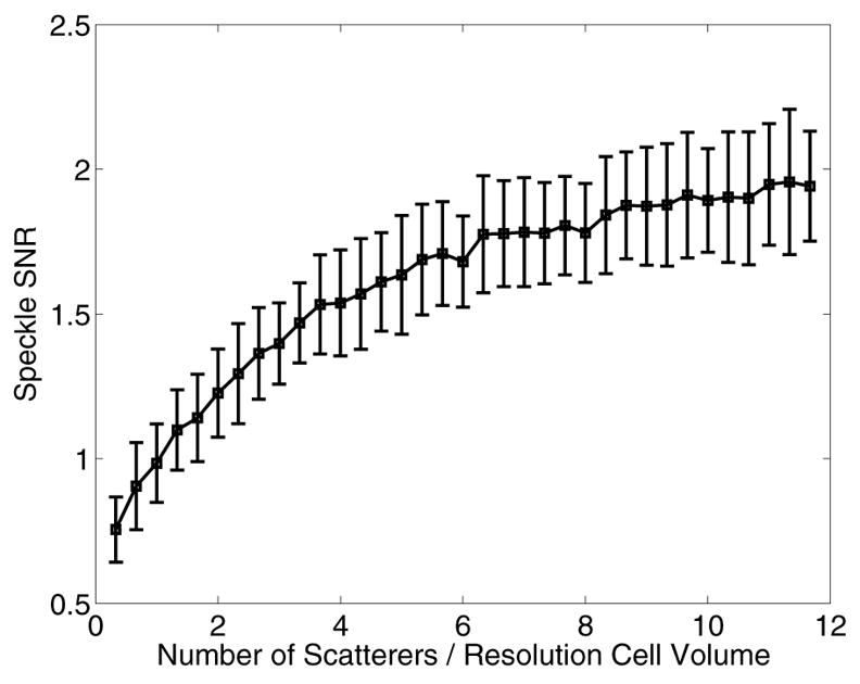
Calculated speckle SNR in the focal zone as a function of the number of scatterers in the −6 dB resolution cell volume of the tracking beam. The theoretical speckle SNR ceiling of 1.91 is approached when approximately 11 scatterers exist per resolution cell volume.

Fig. 2 shows characteristic normalized displacement fields in the axial-lateral plane, centered in elevation, for a material with a Young's modulus of 8.5 kPa and an acoustic attenuation (α) of 0.7 dB/cm/MHz. The top row corresponds to 0.2 ms after initiation of the ARFI excitation (45 μs, F/1.3, 20 mm focal depth), while the center and bottom rows correspond to 1.2 and 2.0 ms respectively. Brighter pixels indicate greater displacement away from the transducer, which is located at the top of each image. The left column shows the FEM simulated displacement fields, while the center column shows those displacement fields after being ultrasonically-tracked at 6.7 MHz, F/0.5 focal configuration on transmit and dynamic receive and a transmit focal depth of 20 mm. The right column shows the corresponding experimental ARFI displacement data in a gelatin phantom [18] with similar acoustic and mechanical parameters to those simulated in the center column. Statistical analysis was performed on the characteristic line plots shown in Fig. 3, representing displacement as a function of depth, centered laterally. The rows in Fig. 3 correspond to the same time steps shown in Fig. 2. The solid lines in the left column (a,d,g) represent the FEM displacement data at the center lateral position, while the dashed line represents the tracked displacement data along these center lines. These dashed lines are repeated in the center column plots (b,e,h) (again representing the same tracked data as in (a,d,g)), while the solid lines in the center column now represent the tracked data after a 3.85 mm kernel running average. The plots in the right column (c,f,i) represent the jitter in the tracked displacement data after the running average data was subtracted from the raw tracked data (solid and dashed lines, respectively, in (b,e,h)). Note that the underestimation of maximum displacement is worse in the early time step (a), and the focal zone jitter is worse immediately after excitation (c) compared with later in time (f,i).

Fig. 2.

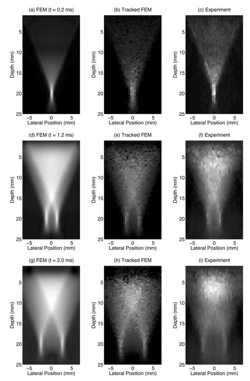
Normalized displacement fields following ARFI excitation for the FEM data (left column), tracked FEM data (center column), and phantom data (right column) for three different time steps (0.2 ms top row, 1.2 ms center row, 2.0 ms bottom row). The modeled material and phantom were 8.5 kPa with an attenuation of 0.7 dB/cm/MHz. Ultrasonic tracking was performed at a center frequency of 6.7 MHz, a transmit focal depth of 20 mm, and an F/0.5 focal configuration on transmit and dynamic receive. The tracked FEM data (center column) has been downsampled to match the experimental data (right column).

Fig. 3.

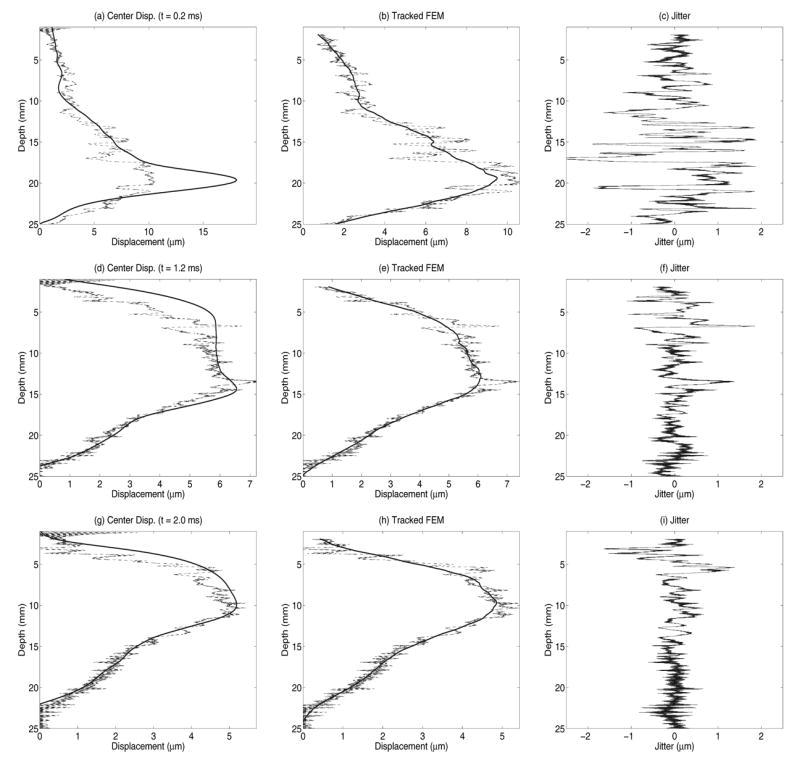
The solid lines in (a,d,g) represent the FEM displacement data, centered laterally, 0.2, 1.2, and 2.0 ms after ARFI excitation, respectively, as was shown in Fig. 2(a,d,g). The dashed line represents the tracked displacement data along these center lines. The dashed lines in (b,e,h) represent the same tracked data as in (a,d,g), while the solid line represents the tracked data after a 3.85 mm kernel running average. The plots in (c,f,i) represent the jitter in the tracked displacement data after the running average data (solid lines) were subtracted from the raw tracked data (dashed lines) in (b,e,h). Note that the underestimation of maximum displacement is worse in the early time step (a), and the focal zone jitter is worse immediately after excitation (c) than later in time (f,i).

Fig. 4 shows how the maximum displacement estimate in the focal zone (a) and the jitter magnitudes over all depths (b) vary as functions of time after the ARFI excitation for materials with Young's moduli of 8.5, 23, and 58 kPa, using the same tracking configuration as described for Figs. 2 and 3.

Fig. 4.

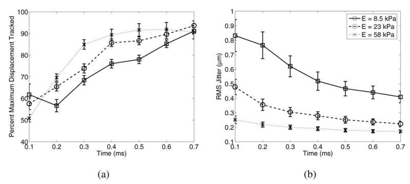
(a) Percentage of maximum displacement tracked in the focal zone in materials with Young's moduli of 8.5, 23, and 58 kPa at times ranging from 0.1 − 0.7 ms after radiation force excitation. Note that accuracy of maximum displacement estimation improves more rapidly for the stiffer material (E = 58 kPa) than for the more compliant media. (b) Jitter decreases with time for all media and is greater in the more compliant media due to greater displacement magnitudes and slower shear wave speeds.

Fig. 5 shows the FEM displacement (solid lines) and tracked displacement (dashed lines) through time at the focal point for 4 (a), 8.5 (b), and 23 kPa (c) materials. No running average was applied to the tracked data in these plots. Figs. 4 and 5 show slightly different estimates for displacement underestimation for the same data since a 3.85 mm running average was applied to the tracked data in the focal zone in Fig. 4, while the focal point data in Fig 5 was not spatially averaged.

Fig. 5.

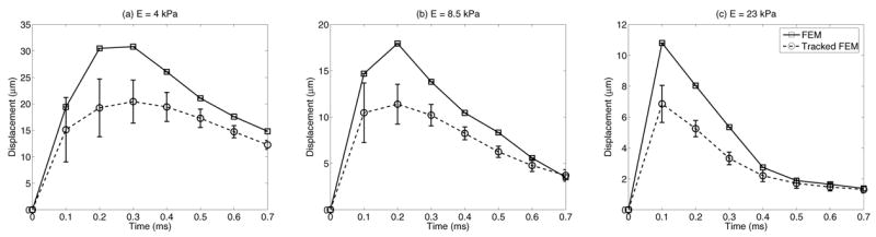
Focal point displacement through time for 4.0 (a), 8.5 (b) and 23 kPa (c) materials. FEM displacement data is represented by the solid lines, while tracked data is represented by the dashed line. No running average was applied to the tracked data. Note that the greater displacement underestimation occurs at the time of peak displacement, while jitter is greatest at the first time step, not the time of peak displacement.

Since biological tissues can be underpopulated by scatterers and may not have fully developed speckle, simulations were run to determine the impact of underdeveloped speckle on displacement estimate accuracy. Fig. 6 shows that underestimation of maximum displacement in the focal zone (a) and jitter magnitude (b) increase as scatterer density decreases.

Fig. 6.

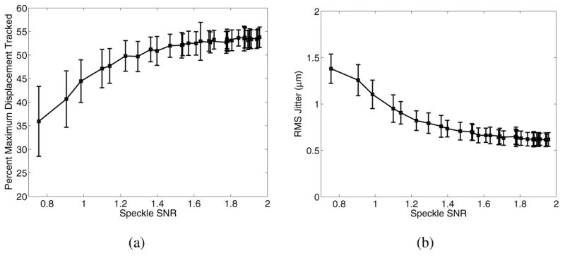
Displacement underestimation (a) and jitter (b) as a function of scatterer density, as represented by speckle SNR. The plot on the left demonstrates that lower speckle SNR is associated with greater displacement underestimation, while the plot on the right shows decreased jitter with higher speckle SNR. Note that fully developed speckle has an SNR of 1.91.

As the CRLB in Eqn. 1 indicates, increasing the frequency of the tracking beams should reduce jitter magnitude. Fig. 7(a–b) shows the accuracy of maximum displacement estimates and jitter with increasing tracking transmit frequency for a transducer with a fixed center frequency of 7.2 MHz and 53% fractional bandwidth, with a fixed 0.35 μs tracking kernel length for all frequencies. To explore the effects of bandwidth on different tracking frequencies, Fig. 7(c–d) shows the same plots for transducers with 53% fractional bandwidth, but with a transducer center frequency at the specified tracking transmit frequency. Again, the tracking kernel length was held at 0.35 μs for all frequencies. The impact of varying the center frequency of the transducer on the lateral transmit/receive beamwidth can be seen in Fig. 8, where (a) shows the beamplots for a fixed 7.2 MHz center frequency, and (b) shows the beamplots for the variable center frequencies. This same transducer configuration is shown in Fig. 7(e–f), except the kernel length was held at 2.5 cycles for each tracking frequency instead of 0.35 μs. The CRLB theoretical curves are shown in the dashed lines in Fig. 7(d,f).

Fig. 7.

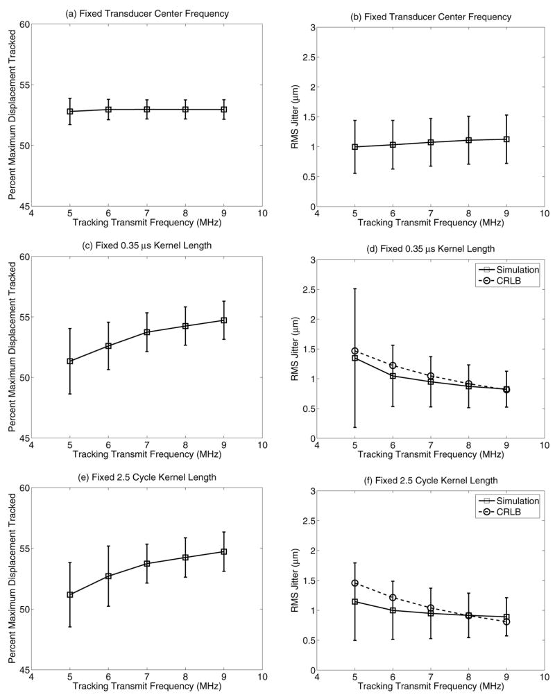
Plots demonstrating the impact of tracking transmit frequency and bandwidth on displacement underestimation (left column) and jitter (right column). The plots in the top row have a fixed transducer center frequency of 7.2 MHz with a fractional bandwidth of 53% and a constant kernel length of 0.35 μs. The center row maintains a fractional bandwidth of 53%, but the transducer center frequency was set to the tracking tracking frequency. The bottom row shows the same configuration as the center row, except the kernel length was fixed at 2.5 cycles instead of a constant 0.35 μs. The CRLB is shown by the dashed line with circles in plots (d) and (f).

Fig. 8.

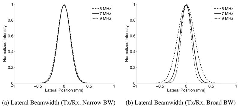
Plots of the lateral transmit/receive (Tx/Rx) beamwidths at the focal depth for a fixed fractional bandwidth of 53%. Plot (a) represents a fixed transducer center frequency of 7.2 MHz, while (b) represents a transducer center frequency that varies with the transmitted frequency. The solid lines represent a transmitted beam at 7 MHz, while the dashed and dotted lines represent frequencies of 5 and 9 MHz respectively. Note that in (a), the beamwidth are almost identical, highlighting the limitation of the fractional bandwidth, which is overcome in (b).

Fig. 9 shows displacement underestimation in the focal zone (a) and jitter (b) in an 8.5 kPa material where the force magnitude was scaled to achieve the maximum displacement values (at the focal point) shown on the abscissa.

Fig. 9.

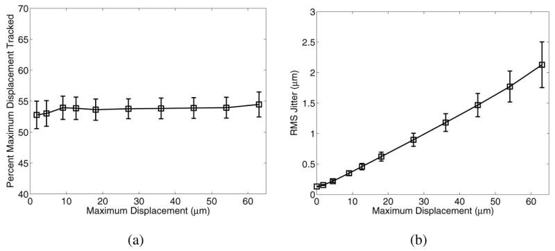
Plot (a) shows that the relative displacement underestimation is not significantly affected by the magnitude of the displacement field, while plot (b) shows that for larger displacements, jitter is directly related to displacement magnitude.

The impact of using different F/#s for the track beams was evaluated for an unapodized F/1 excitation configuration. Fig. 10 shows the displacement underestimation (a) and jitter (b) immediately after excitation for apodized track beams of varying transmit/receive track F/# configurations.

Fig. 10.

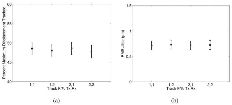
Displacement underestimation (a) and jitter (b) immediately after excitation with an F/1 excitation configuration for varying transmit (Tx) / receive (Rx) F/# combinations used for the tracking beams.

Fig. 11 shows the displacement profiles in the lateral dimension for materials with Young's moduli of 1 (top row), 8.5 (middle row) and 23 kPa (bottom row) for F/1 and F/2 excitation focal configurations, 0.1 ms after excitation. Fig. 11(a) shows the lateral beamwidth of the ARFI excitation beams (which are not apodized). The left and center columns compare the lateral beamwidths of the excitation beams (dashed lines) relative to the simulated displacement profiles (solid lines) in the lateral dimension for F/1 and F/2 excitations, respectively. The right column shows the comparison of the simulated F/1 (solid) and F/2 (dashed) displacement profiles. Note that as the media stiffness increases, the displacement profiles for the F/1 and F/2 excitations 0.1 ms after excitation become very similar (g,j).

Fig. 11.

Displacement profiles in the lateral dimension for materials with Young's moduli of 1 (top row), 8.5 (middle row) and 23 kPa (bottom row) for F/1 and F/2 excitation focal configurations, 0.1 ms after the ARFI excitation. Plot (a) shows the lateral beamwidth of the ARFI excitation beams (which are not apodized). The left and center columns show comparisons of the lateral excitation beamwidths (dashed) relative to the resulting displacement profiles 0.1 ms after excitation (solid) in the lateral dimension for F/1 and F/2 excitations, respectively, while the right column shows the comparison of the F/1 (solid) and F/2 (dashed) displacement profiles. Note that the displacement profiles are more similar between F/1 and F/2 excitation configurations in the stiffer media at this time due to the faster shear wave speed (g,j).

Fig. 12 shows the impact that using broader excitation F/# focal configurations has on the displacement underestimation (a) and jitter (b) 0.2 ms after excitation in a 4 kPa. The tracking transmit and receive focal configurations were held at F/1 for all excitation configurations.

Fig. 12.

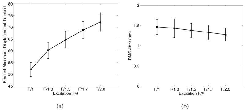
This figure shows the reduction in displacement underestimation (a) when using higher excitation F/# focal configurations, while not significantly affecting the jitter levels (b). The tracking F/# focal configuration was F/1 for both transmit and receive, and the material was modeled with a Young's modulus of 4 kPa.

In applications of ARFI imaging where multiple focal depths for excitation are employed, it is experimentally advantageous to maintain a constant tracking transmit focal depth [26]. Fig. 13 shows how displacement underestimation (a) and jitter (b) 0.2 ms after excitation vary as a function of tracking transmit focal depth for an ARFI excitation focused at 10 mm in an 8.5 kPa material.

Fig. 13.

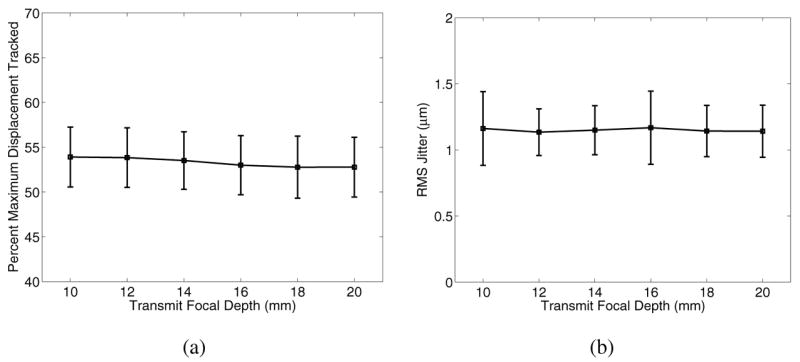
Displacement estimation accuracy (a) and jitter (b) as a function of tracking focal depths deep to the excitation focal depth, 0.2 ms after excitation with an F/1.3 focal configuration in an 8.5 kPa material. In this case, the excitation focal depth was 10 mm, while the transmit focal depth on tracking was varied from 10 – 20 mm, always using dynamic receive focusing.

To evaluate the impact of axial shearing within the tracking kernel, the data presented in Fig. 2 and 3 was tracked using kernel lengths of 0.17 μs (1.25 cycles) and 0.70 μs (5 cycles), and compared with the standard 0.35 μs (2.5 cycle) kernel length, as shown in Fig. 14.

Fig. 14.

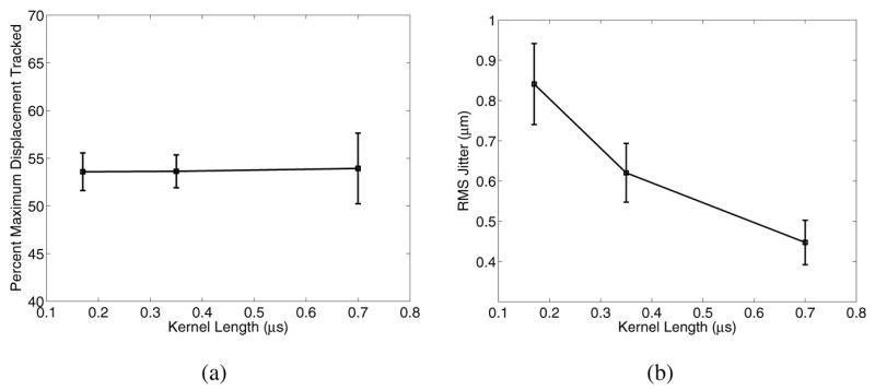
Displacement underestimation (a) and jitter (b) 0.2 ms after excitation for varying kernel lengths in an 8.5 kPa material. Note that the larger kernel length reduces the jitter, but for the sizes evaluated, the kernel length does not impact the accuracy of the displacement estimate.

V. Discussion

Displacement underestimation and jitter in ultrasonic cross-correlation estimated displacements (Fig. 3) is significant, where up to a 50% displacement underestimation can occur within the focal zone. As previous work by McAleavey et al. [22] and the simulation results presented herein have shown, this is attributed to scatterer shearing in the lateral and elevation dimensions. This underestimation is dependent on material stiffness because shear wave propagation reduces shearing in the lateral and elevation dimensions relative to the track beam PSF, and this occurs more quickly for higher shear wave speeds (i.e., stiffer media). This result is confirmed in Fig. 4, where in the stiffer medium (58 kPa) tracking accuracy improves sooner after excitation than in the more compliant media. Fig. 4 also shows that the more compliant medium (E = 8.5 kPa) suffers from greater displacement underestimation later in time (0.2 ms), concurrent with the later peak displacement in this more complaint media, as shown in Fig. 5. Also notice in Fig. 4(b) and Fig. 5 that while the greatest displacement underestimation occurs at the time of peak displacement, the greatest jitter occurs at the first time step after excitation, independent of the material stiffness, and the jitter is greater for the more compliant media. Fig 3(a,c) also shows that the greatest displacement underestimation and jitter occur in the focal zone, where shearing and displacement magnitude are the greatest. This indicates that jitter is a function of the displacement magnitude (Fig. 9(b)) and the amount of shearing under the track PSF as dictated by shear wave propagation away from the ROE.

Jitter increases with greater displacement magnitude, consistent with the findings of McAleavey et al. [22], and is due to a lower correlation coefficient during tracking. Displacement magnitude, however, does not appreciably change the relative amount of displacement underestimation that occurs, as shown in Fig. 9(a), which is again consistent with the findings of McAleavey et al. [22].

Greater signal decorrelation also occurs in the presence of underdeveloped speckle, and as shown in Fig. 6, resulting in greater displacement underestimation and jitter. Biological tissues, such as breast tissue, do not always exhibit fully developed speckle [39]. Even within a single field-of-view (FOV), structures of varying scatterer density may be present that could impact the relative accuracy of displacement tracking within those structures (e.g., fat versus muscle versus connective tissue). This would be most evident in the in vivo setting, where tissues such as the breast can be very heterogeneous.

Given that shearing impacts the degree of displacement underestimation in the focal zone, it would be expected that using broader excitation beams relative to the tracking beams would reduce this underestimation, which is shown in Fig. 12 where improved tracking accuracy is achieved by using higher F/# excitation focal configurations. In contrast to the anticipated improvement in displacement tracking with more tightly focused track beams, Fig. 10(a) shows that using an F/1 versus an F/2 tracking focal configuration does not provide a tracking benefit. Further insight is provided by the results in Fig. 11. Fig. 11(a) demonstrates that, as expected, the F/2 excitation beamwidth is broader in the lateral dimension than the F/1 excitation beamwidth; however, as comparison of the associated displacement profiles shows (d,g,j,m), the −6 dB displacement widths become increasingly similar with increasing stiffness (right column, Fig. 11). This is caused by lateral displacement profile broadening with time after excitation at a rate that is dictated by the shear wave speed. Therefore, considerable tracking improvement is possible by using broader F/# focal configurations on the excitation beam (Fig. 12). The modeled transducers had a fixed elevation focus, but the use of 1.5D or 2D arrays to control the elevation beamwidth in a similar manner to the lateral beamwidth would also improve displacement tracking accuracy by reducing shearing in the elevation dimension.

The benefits of increasing the tracking frequency, as predicted by the CRLB (Eqn. 1), are only fully evident if the transducer has adequate bandwidth to take advantage of the higher excitation frequency. As shown in Fig. 8(a), a fractional bandwidth of 53% does not allow the transducer to effectively operate at frequencies other than the center frequency. This was evident in Fig. 7(a–b), where there were no appreciable differences in tracking accuracy and jitter when using different tracking frequencies. By changing the center frequency to match the tracking frequency, as shown in Fig. 8(b), the changes in beamwidth that are expected with changing frequency (lateral beamwidth ≃ λ x F/#) are now evident and the anticipated improvements in tracking are apparent in Fig 7(c–d). These tracking improvements could be achieved in practice with a single higher bandwidth transducer.

The fixed kernel length of 0.35 μs in these plots caused larger variances for the lower frequencies where fewer number of cycles were included in each kernel as compared with the higher track frequencies. By holding a fixed 2.5 cycles per kernel, as is done experimentally, the jitter variances for the lower frequencies improved, as shown in Fig. 7(f). This occurs because more samples are fed into the correlation algorithm when compared with the fixed 0.35 μs kernel length that includes 3.2 cycles at 9 MHz versus 1.8 cycles at 5 MHz.

The lower mean jitter predicted by the simulations compared with the CRLB (Fig. 7(d,f)) was unexpected. However, these trends have been reported in the literature and are attributed to the fact that the CRLB does not take into account a biased estimator, which can lead to lower jitter than predicted by CRLB in the case of displacement underestimation [32].

Experimentally, it is advantageous to use a single track focal depth when multiple excitation focal depths are used for ARFI imaging, as is described by Nightingale et al. [26]. Tracking displacement deeper than the excitation focal depth is also advantageous to observe mechanical wave propagation and displacement fields that are generated deeper than the excitation focal depth. As Fig. 13 shows, there is no penalty in using a deeper focal depth on track than on excitation. This is made possible by the use of dynamic receive to modify the receive focal configuration, and therefore the receive beamwidth, remains constant as a function of depth.

Fig. 14(a) demonstrates that the minimal axial shearing that occurs within the kernel lengths used for ARFI displacement tracking does not appreciably impact tracking accuracy. Jitter, however, was improved (Fig. 14(b)) due to improved correlation achieved by using larger data ensembles in the correlation algorithms.

The FEM displacement field shown in Fig. 2(a) does not exhibit near-field interference patterns that would be expected in the pressure fields generated during the ARFI excitations. The Field II output does reflect these interference patterns, as shown in Palmeri et al. [31]; however the continuum nature of the tissue and the spatial gradients present due to the excitation focal configurations cause the loss of these interference patterns before the first experimentally tracked time step. Therefore, the displacement variations present in the near-field in the tracked simulation and experimental data should not be mistaken for these interference patterns, but are attributed to the jitter associated with the displacement tracking algorithms.

VI. Conclusions

These simulation studies have demonstrated that lateral and elevation scatterer shearing within the track PSF causes a significant underestimation in tissue displacement estimates in response to ARFI excitations. Axial shearing is not significant over the kernel lengths typically used in ARFI imaging. Jitter increases with increasing tissue displacement and increasing lateral and elevation shearing due to decreased correlation coefficients. Displacement underestimation and jitter decrease with time after the ARFI excitation as shear waves propagate away from the ROE, reducing the amount of shearing within the tracking PSF. In stiffer media with higher shear wave speeds, this improvement occurs sooner than in more compliant media. Using higher F/# excitations leads to less lateral shearing within the tracking beams and greater displacement tracking accuracy. Displacement underestimation and jitter are higher in materials with underdeveloped speckle (SNR <1.91). The use of higher tracking frequencies in high-bandwidth transducers will result in decreased jitter and reduced displacement underestimation. The use of 2D focusing in the elevation dimension will also improve displacement tracking accuracy. Finally, there is no loss in tracking accuracy when using a transmit track focus deeper than the ARFI excitation focus in the presence of dynamic receive focusing.

References

- 1.Bercoff J, Tanter M, Fink M. Supersonic shear imaging: A new technique for soft tissue elasticity mapping. IEEE Trans Ultrason, Ferroelec, Freq Contr. 2004;51(4):396–409. doi: 10.1109/tuffc.2004.1295425. [DOI] [PubMed] [Google Scholar]
- 2.Bilgen M, Insana MF. Error analysis in acoustic elastography. ii. strain estimation and snr analysis. J Acoust Soc Am. 1997;101(2):1147–54. doi: 10.1121/1.418019. [DOI] [PubMed] [Google Scholar]
- 3.Bilgen M, Insana MF. Elastostatics of a spherical inclusion in homogeneous biological media. Phys Med Biol. 1998;43(1):1–20. doi: 10.1088/0031-9155/43/1/001. [DOI] [PubMed] [Google Scholar]
- 4.Bohs L, Friemel B, McDermott B, Trahey G. A realtime system for quantifying and displaying two-dimensional velocities using ultrasound. Ultrasound Med Biol. 1993;19(9):751–761. doi: 10.1016/0301-5629(93)90092-3. [DOI] [PubMed] [Google Scholar]
- 5.Bonnefous O, Pesque P. Time domain formulation of pulse-doppler ultrasound and blood velocity estimation by cross correlation. Ultrasonic Imaging. 1986;8:73–85. doi: 10.1177/016173468600800201. [DOI] [PubMed] [Google Scholar]
- 6.Carter G. Coherence and time delay estimation. IEEE Trans Ultrason, Ferroelec, Freq Contr. 1987;75(2):236–255. [Google Scholar]
- 7.Céspedes E, de Korte C, van der Steen A. Echo decorrelation from displacement gradients in elasticity and velocity estimation. IEEE Trans Ultrason, Ferroelec, Freq Contr. July 1999;46(4):791–801. doi: 10.1109/58.775642. [DOI] [PubMed] [Google Scholar]
- 8.Cespedes I, Insana M, Ophir J. Theoretical bounds on strain estimation in elastography. IEEE Trans Ultrason, Ferroelec, Freq Contr. 1995;42(5):969–72. [Google Scholar]
- 9.Chaturvedi P, Insana M, Hall T. 2-d companding for noise reduction in strain imaging. IEEE Trans Ultrason, Ferroelec, Freq Contr. 1998;45(1):179–191. doi: 10.1109/58.646923. [DOI] [PubMed] [Google Scholar]
- 10.Chaturvedi P, Insana M, Hall T. Testing the limitations of 2-d companding for strain imaging using phantoms. IEEE Trans Ultrason, Ferroelec, Freq Contr. 1998;45(4):1022–1031. doi: 10.1109/58.710585. [DOI] [PubMed] [Google Scholar]
- 11.Embree P, O'Brien W. Volumetric blood flow via time-domain correlation: experimental verification. IEEE Trans Ultrason, Ferroelec, Freq Contr. 1990;37:176–189. doi: 10.1109/58.55307. [DOI] [PubMed] [Google Scholar]
- 12.Fatemi M, Greenleaf J. Ultrasound-stimulated vibro-acoustic spectrography. Science. 1998;280:82–85. doi: 10.1126/science.280.5360.82. [DOI] [PubMed] [Google Scholar]
- 13.Fatemi M, Greenleaf J. Probing the dynamics of tissue at low frequencies with the radiation force of ultrasound. Phys Med Biol. 2000;45(6):1449–1464. doi: 10.1088/0031-9155/45/6/304. [DOI] [PubMed] [Google Scholar]
- 14.Friemel B, Bohs L, Nightingale K, Trahey G. Speckle decorrelation due to two-dimensional flow gradients. IEEE Trans Ultrason, Ferroelec, Freq Contr. 1998;45(2):317–327. doi: 10.1109/58.660142. [DOI] [PubMed] [Google Scholar]
- 15.Fu D, Levinson S, Gracewski S, Parker K. Noninvasive quantitative reconstruction of tissue elasticity using an iterative forward approach. Phys Med Biol. 2000;45(6):1495–1509. doi: 10.1088/0031-9155/45/6/307. [DOI] [PubMed] [Google Scholar]
- 16.Goodman J. Introduction to Fourier Optics. McGraw-Hill; New York: 1996. [Google Scholar]
- 17.Hall T, Zhu Y, Spalding C. In vivo real-time freehand palpation imaging. Ultrasound Med Biol. 2003;29(3):427–435. doi: 10.1016/s0301-5629(02)00733-0. [DOI] [PubMed] [Google Scholar]
- 18.Hall TJ, Bilgen M, Insana MF, Krouskop TA. Phantom materials for elastography. IEEE Trans Ultrason, Ferroelec, Freq Contr. 1997;44(6):1355–65. [Google Scholar]
- 19.Jensen J, Svendsen N. Calculation of pressure fields from arbitrarily shaped, apodized, and excited ultrasound transducers. IEEE Trans Ultrason, Ferroelec, Freq Contr. 1992;39(2):262–267. doi: 10.1109/58.139123. [DOI] [PubMed] [Google Scholar]
- 20.Konofagou E, Thierman J, Hynynen K. A focused ultrasound method for simultaneous diagnostic and therapeutic applications–a simulation study. Phys Med Biol. Nov 2001;46(11):2967–2984. doi: 10.1088/0031-9155/46/11/314. [DOI] [PubMed] [Google Scholar]
- 21.Lizzi F, Muratore R, Deng C, Ketterling J, Alam K, Mikaelian S, Kalisz A. Radiation-force technique to monitor lesions during ultrasonic therapy. Ultrasound Med Biol. 2003;29(11):1593–1605. doi: 10.1016/s0301-5629(03)01052-4. [DOI] [PubMed] [Google Scholar]
- 22.McAleavey S, Nightingale K, Trahey G. Estimates of echo correlation and measurement bias in acoustic radiation force impulse imaging. IEEE Trans Ultrason, Ferroelec, Freq Contr. 2003;50(6):631–641. doi: 10.1109/tuffc.2003.1209550. [DOI] [PubMed] [Google Scholar]
- 23.McKnight A, Kugel J, Rossman P, Manduca A, Hartmann L, Ehman R. MR elastography of breast cancer: Preliminary results. AJR. 2002;178(6):1411–1417. doi: 10.2214/ajr.178.6.1781411. [DOI] [PubMed] [Google Scholar]
- 24.Nightingale K, Bentley R, Trahey G. Observations of tissue response to acoustic radiation force: Opportunities for imaging. Ultrasonic Imaging. 2002;24:100–108. doi: 10.1177/016173460202400301. [DOI] [PubMed] [Google Scholar]
- 25.Nightingale K, Palmeri M, Nightingale R, Trahey G. On the feasibility of remote palpation using acoustic radiation force. J Acoust Soc Am. 2001;110(1):625–634. doi: 10.1121/1.1378344. [DOI] [PubMed] [Google Scholar]
- 26.Nightingale K, Palmeri M, Trahey G. Analysis of contrast in images generated with transient acoustic radiation force. Ultrasound Med Biol. 2006;32(1):61–72. doi: 10.1016/j.ultrasmedbio.2005.08.008. [DOI] [PubMed] [Google Scholar]
- 27.Nyborg W. Acoustic streaming. In: Mason W, editor. Physical Acoustics. IIB. Academic Press Inc; New York: 1965. pp. 265–331. chapter 11. [Google Scholar]
- 28.O'Donnell M, Skovoroda A, Shapo B, Emelianov S. Internal displacement and strain imaging using ultrasonic speckle tracking. IEEE Trans Ultrason, Ferroelec, Freq Contr. 1994;41:314–325. [Google Scholar]
- 29.Oliphant T, Manduca A, Ehman R, Greenleaf J. Complex-valued stiffness reconstruction fro magnetic resonance elastography by algebraic inversion of the differential equation. Magnetic Resonance in Medicine. 2001;45:299–310. doi: 10.1002/1522-2594(200102)45:2<299::aid-mrm1039>3.0.co;2-o. [DOI] [PubMed] [Google Scholar]
- 30.Ophir J, Alam S, Garra B, Kallel F, Konofagou E, Krouskop T, Varghese T. Elastography: Ultrasonic estimation and imaging of the elastic properties of tissue. Proc Inst Mech Engrs. 1999;213:203–233. doi: 10.1243/0954411991534933. [DOI] [PubMed] [Google Scholar]
- 31.Palmeri M, Sharma A, Bouchard R, Nightingale R, Nightingale K. A finite-element method model of soft tissue response to impulsive acoustic radiation force. IEEE Trans Ultrason, Ferroelec, Freq Contr. 2005;52(10):1699–1712. doi: 10.1109/tuffc.2005.1561624. [DOI] [PMC free article] [PubMed] [Google Scholar]
- 32.Pinton G, McAleavey S, Dahl J, Nightingale K, Trahey G. Real-time acoustic radiation force impulse imaging. Proceedings of the 2005 SPIE Conference on Medical Imaging; 2005. [Google Scholar]
- 33.Plewes D, Bishop J, Samani A, Sciarretta J. Visualization and quantification of breast cancer biomechanical properties with magnetic resonance elastography. Phys Med Biol. 2000;45(1):1591–1610. doi: 10.1088/0031-9155/45/6/314. [DOI] [PubMed] [Google Scholar]
- 34.Sarvazyan A, Rudenko O, Swanson S, Fowlkes J, Emelianov S. Shear wave elasticity imaging: A new ultrasonic technology of medical diagnostics. Ultrasound Med Biol. 1998;24(9):1419–1435. doi: 10.1016/s0301-5629(98)00110-0. [DOI] [PubMed] [Google Scholar]
- 35.Sinkus R, Lorenzen J, Schrader D, Lorenzen M, Dargatz M, Holz D. High-resolution tensor MR elastography for breast tumour detection. Phys Med Biol. 2000;45(6):1649–1664. doi: 10.1088/0031-9155/45/6/317. [DOI] [PubMed] [Google Scholar]
- 36.Steele D, Chenevert T, Skovoroda A, Emelianov S. Three-dimensional static displacement, stimulated echo NMR elasticity imaging. Phys Med Biol. 2000;45(1):1633–1648. doi: 10.1088/0031-9155/45/6/316. [DOI] [PubMed] [Google Scholar]
- 37.Sugimoto T, Ueha S, Itoh K. Tissue hardness measurement using the radiation force of focused ultrasound; Proceedings of the 1990 Ultrasonics Symposium; 1990. pp. 1377–1380. [Google Scholar]
- 38.Taylor L, Porter B, Rubens D, Parker K. Three-dimensional sonoelastography: Principles and practices. Phys in Med Biol. 2000;45:1477–1494. doi: 10.1088/0031-9155/45/6/306. [DOI] [PubMed] [Google Scholar]
- 39.Tohno E, Cosgrove D, Sloane J. Ultrasound Diagnosis of Breast Diseases. Churchill Livingstone Inc., 650 Avenue of the Americas; New York, NY 10011: 1994. [Google Scholar]
- 40.Van Houten E, Weaver J, Miga M, Kennedy F, Paulsen K. Elasticity reconstruction from experimental MR displacement data: initial experience with an overlapping subzone finite element inversion process. Medical Physics. 2000;27(1):101–107. doi: 10.1118/1.598861. [DOI] [PubMed] [Google Scholar]
- 41.Varghese T, Zagzebski J, Lee F. Elastographic imaging of thermal lesions in the liver in vivo following radiofrequency ablation: Preliminary results. Ultrasound Med Biol. 2002;28:1467–1473. doi: 10.1016/s0301-5629(02)00656-7. [DOI] [PubMed] [Google Scholar]
- 42.Viola F, Walker W. A comparison of the performance of time-delay estimators in medical ultrasound. IEEE Trans Ultrason, Ferroelec, Freq Contr. 50(4):392–401. doi: 10.1109/tuffc.2003.1197962. [DOI] [PubMed] [Google Scholar]
- 43.Walker W, Fernandez F, Negron L. A method of imaging viscoelastic parameters with acoustic radiation force. Phys Med Bio. 2000;45(6):1437–1447. doi: 10.1088/0031-9155/45/6/303. [DOI] [PubMed] [Google Scholar]
- 44.Walker W, Trahey G. A fundamental limit on delay estimation using partially correlated speckle signals. IEEE Trans Ultrason, Ferroelec, Freq Contr. 1995;42(2):301–308. [Google Scholar]