

Abstract
Pixel saturation, where the incident light at a pixel causes one of the color channels of the camera sensor to respond at its maximum value, can produce undesirable artifacts in digital color images. We present a Bayesian algorithm that estimates what the saturated channel's value would have been in the absence of saturation. The algorithm uses the non-saturated responses from the other color channels, together with a multivariate Normal prior that captures the correlation in response across color channels. The appropriate parameters for the prior may be estimated directly from the image data, since most image pixels are not saturated. Given the prior, the responses of the non-saturated channels, and the fact that the true response of the saturated channel is known to be greater than the saturation level, the algorithm returns the optimal expected mean square estimate for the true response. Extensions of the algorithm to the case where more than one channel is saturated are also discussed. Both simulations and examples with real images are presented to show that the algorithm is effective.
1. Introduction
In digital imaging we are often confronted with the problem of pixel saturation. Consider the case of an RGB (red, green, and blue) color camera with 8-bit quantization. An R, G, or B pixel value is saturated when it takes on its maximum value, in this case 255. When pixels are saturated, information about the scene is lost, since we have only a lower bound on the sensor response that would have occurred in the absence of saturation. Moreover, if not handled carefully, saturated pixels can lead to image artifacts. These can be particularly salient in color imaging where saturation in one color channel changes the relative RGB values. This is likely to occur when the illuminant has a strong color cast or when the camera design includes large differences in gain for the different color channels. Saturation of responses to image highlights, which tend to be achromatic, can be particularly noticeable.
Although saturated pixels can be avoided by appropriate choice of exposure duration and lens f-stop, in practice they occur quite often. Indeed, reducing exposure duration or stopping down to the point where no pixels are saturated can result in unacceptable images: in scenes containing a small number of locations with very high intensities, for example, eliminating all saturation forces most of the image to occupy only a small portion of the available quantization levels.
To understand the effect of pixel saturation, it is important to remember that raw camera RGB values are not generally suitable for direct display on a monitor. Rather, these RGB values must be processed for display (or printing).1, 2 Practical implementations of image processing pipelines vary, but operations typically performed include linearization, white balancing, demosaicing, correction for camera spectral sensitivities, conversion between camera and monitor RGB, tone/gamut-mapping, and display gamma correction.3 The detailed nature of artifacts caused by pixel saturation will vary with the particulars of the processing applied, and these in turn will depend on the underlying design of the camera sensors. With this caveat in mind, it is none-the-less informative to illustrate the effects of pixel saturation for a specific camera and simple processing pipeline. Although alternative demosaicing,4-7 color correction,8, 9 and tone mapping10, 11 algorithms may be used at each step, the basic effects illustrated are general.
Fig. 1 shows three renderings of an image acquired with a Kodak DCS200 camera. In the 575×533 raw mosaiced image, 12.6% of the green sensor (G) pixels were saturated, 2.8% of the red sensor (R) pixels were saturated, and less than 0.01% (3 pixels total) of the blue sensor (B) pixels were saturated. A total of 2.4% of the pixels had both red and green sensors saturated. The rendering in the top panel was made by passing the raw sensor values through an image processing pipeline that provides no correction for the saturated pixels. This image was processed as follows:
Bilinear demosacing was applied to the linear raw rgb values to obtain a full color image. Note that mosaicing artifacts are not salient in this image, so that the use of a simple demosaicing algorithm suffices.
The image was white-balanced by applying multiplicative gains to the R and B channels. After the gains were applied the RGB values corresponding to lights with the chromaticity of the scene illuminant had the property that R=G=B, for non-saturated pixels. We measured the scene illuminant with a spectral radiometer when the image was acquired, and used this measurement to set the white balance point.
The white balanced image was color corrected into the sRGB display space (http://www.srgb.com). This was done using a 3×3 matrix obtained using the “maximum ignorance with positivity method” together with measurements of the camera's sensor spectral sensitivities and knowledge of the spectrum of the scene illuminant.12
The sRGB values obtained in step 3 were tone-mapped into the monitor gamut. This corresponds to the range 0-1 for each monitor primary. Negative values were clipped to zero. The remaining values were then multiplied a scale factor equal to 1/5*mg, where mg is the mean value of the green color channel. All scaled display RGB values greater than 1 were then clipped to 1.
The sRGB gamma correction was applied to yield 8-bit RGB values for display.
Fig. 1.
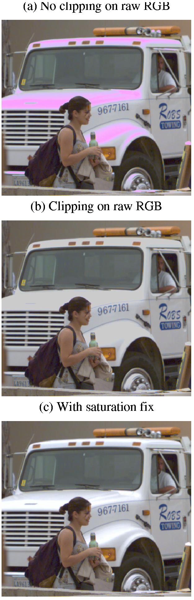
A Kodak DCS200 image rendered without any saturation fix (a), with pixel value clipping to a known white point (b), and with saturation fix (c) for an image with a large number of saturated pixels.
Note the objectionable magenta artifacts on the bright white areas of the truck. Fundamentally, these occur because of saturation of the G sensor responses for these image regions. This saturation leaves the response of the G sensor for these regions lower than it should be, relative to the non-saturated responses of the R and B sensors. After color balancing, the effect of this relative decrease in G sensor response is a shift of the rendered color towards magenta.
The artifacts such as those seen in the top panel of Fig. 1 are not commonly observed in rendered images produced by commercial digital cameras. A simple approach that reduces the saliance of the artifacts is to introduce a clipping step into the processing pipeline, after white balancing and before color correction. After the white balancing gains are applied, R and B sensor responses that are above the maximum sensor response are clipped to this maximum value. Since no gain is applied to the G channel during white balancing, the G values do not require clipping. The clipping operation has the effect of forcing R=G=B for most saturated image regions. This is the white balance point of the rendered image.
Fig. 1(b) shows the result of reprocessing the truck image with the addition of the clipping operation. For this image, clipping provides an effective fix for the colored artifacts that arise from pixel saturation. On the other hand, clipping throws away information, as pixels that originally differ in the image are mapped to the same rendered values after the clipping step. This information loss may be seen on the trunk and fender of the truck in Fig. 1(b), where the lack of variation across large regions gives an unnatural appearance to the truck. Note that information about the variation is in fact available in the raw sensor image, since the responses of non-saturated color channels do vary across regions where some channels are saturated.
In practice, each camera manufacturer adopts its own proprietary method for reducing the effects of pixel saturation, and the details of the algorithms are not in the public domain. Informal conversations with colleagues and examination of images produced by cameras, however, indicate that some form of clipping operation similar to that illustrated above is at the heart of current practice. This clipping operation is usually done to keep pixel values within the number of bits represented on the hardware, and not specifically to deal with pixel saturation. Nevertheless, it has the beneficial side effect of eliminating most color artifacts that would have arisen from pixel saturation, at the cost of some lost information in highlight areas of an image.
Here we present a novel method to handle saturated pixel values. The method is based on the intuition that in regions where some sensor channels are saturated, the non-saturated channels continue to provide useful information. In particular, there is in general a strong correlation between pixel values in the different sensor channels, so that non-saturated values at an image location carry information that may be used to correct a saturated value at the same location. If the G pixel value is saturated but the R and B values are not, for example, then the R and B values may be used to estimate what we refer to as the true value of the G pixel, that is the value that would have been registered in the absence of saturation.
Our method is based on the principles of Bayesian estimation, a general approach that has been widely used to develop image processing algorithms.6, 13-15 Since the algorithm operates on the raw sensor responses, it is intended to be incorporated into the camera image processing pipeline and is not appropriate for post-processing already rendered images. The algorithm is the subject of a US Patent.16 The bottom image in Fig. 1 shows the example image processed with the algorithm presented in this paper. The color artifacts are removed without the loss of shading information that occurs with clipping.
2. Saturation fix algorithm
The general Bayesian framework for estimation is well-known.17, 18 Here we develop the ideas specifically in the context of estimating the true value of a saturated pixel. Central to the Bayesian approach is the notion of using prior information. Here the relevant prior information is the joint distribution of RGB values, which we characterize by a multivariate Normal distribution. Such prior distributions have been used previously in color image processing.6, 13, 19 Although they fall short of capturing all of the statistical structure of natural images, they do allow us to express quantitatively the fact that there is a high correlation between the responses of different color channels at each pixel. Fig. 2 shows the R pixel values plotted against the G pixel values (after demosaicing) for 500 non-saturated pixels randomly selected from a portion of the truck image shown in Fig. 1(a). The level of correlation between pixel types is dependent on sensor sensitivity and scene content, and varies between 0.70 and 0.99 for the images we have analyzed. In the case of an n-color camera, the prior distribution of the camera sensor outputs can be characterized as a n-dimensional normal distribution with mean μ = (μ1,μ2,…μn)T and an n × n covariance matrix S.
Fig. 2.
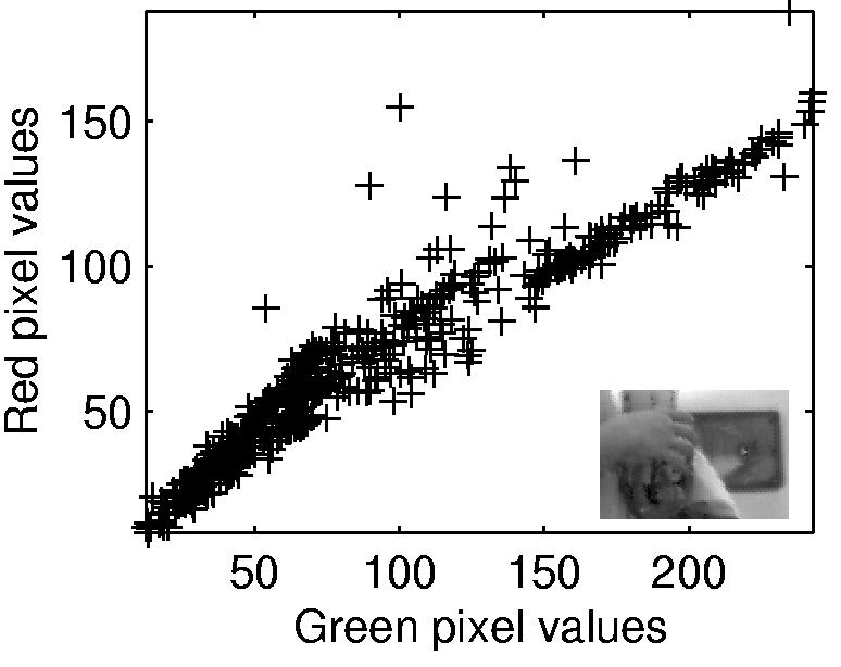
A plot of Red vs Green sensor values for 500 non-saturated pixels randomly selected from an image (shown at lower right corner) after bilinear demosaicing. This image is a sub-region of the truck image in Fig.1(a). The correlation between the R and G values for this image area is 0.96. The RG correlation for the full image in Fig.1(a) is higher (0.99) because the content of that image is largely achromatic.
To simplify explanation of the saturation algorithm, we first assume that the image we start with is either full-color, or has been demosaiced (with the constraint that the demo-saicing process only fills in sensor values missing in the raw image and does not alter the raw pixel values). Therefore, for any pixel location, we have n = ns+nk sensor values representing different color elements at the pixel, ns of which are saturated and nk of which are not saturated. Let us represent the “true” color values of the saturated sensors by an ns × 1 column vector Xs, and the “true” color values of the non-saturated sensors by an nk × 1 column vector Xk. The prior distribution of the sensor values can now be represented as:
| (1) |
whereμs and μk are the expected values of Xs and Xk, Ss and Sk are the covariance matrices of Xs and Xk, Ssk represents the covariance between Xs and Xk, and Sks = SskT. The means and covariances in Eq. (1) are obtained directly from the prior mean μ and covariance S.
Since we are only interested in estimating Xs, we can simplify the calculations significantly by expressing the prior distribution only as a distribution of Xs, conditional on the observed values of the non-saturated sensors Yk, which is determined by Xk plus a random error term ek (Yk = Xk + ek), where ek is a column vector with independent and identically distributed noise elements e ∼ N (0, σe. The joint distribution of Xs and Yk is:
| (2) |
where Sek is an nk × nk diagonal matrix with identical diagonal elements σe.
Given that we know Yk = k, where k is a column vector representing the observed values of Yk, the conditional distribution of Xs is Normal with a mean vector μxs and covariance matrix Sxs:20
| (3) |
It can be proven that the conditional distribution's variance Sxs is always smaller than the original variance Ss if Xs is not independent of Yk.20 Thus when the sensor values of a pixel are correlated, knowledge of the non-saturated sensor values reduces uncertainty of the value of the saturated sensors.
The formulation above is standard, and has been used in both demosaicing19 and color correction21 applications. In the case of saturation, however, we have the additional information that the true values for the saturated sensors are greater than or equal to the saturation level s. We can take advantage of this information. Given that the saturated sensor values are constrained by Ys = Xs + es ≥ s, we find the posterior distribution of Xs subject to this constraint, and given the non-saturated sensor values Yk = k at the same location:
| (4) |
The conditioning on Yk = k can be dropped from the factor that originates as P(Ys ≥ s|Yk = k,Xs = x) because given Xs = x, the only randomness originates with the sensor noise es, and this is independent of the non-saturated sensor values. The other factors remain conditional upon Yk = k, however, as they are not conditioned on Xs.
Eq. (4) is the posterior distribution for the saturated pixel values. The equation contains three factors. The first, P(es ≥s−x), is determined directly by the magnitude for the sensor noise. The second, P(Xs = x|Yk = k), is given by N(μxs,Sxs) from Eq. (3) above. The final factor in the denominator of Eq. (4), P(Ys ≥ s|Yk = k), is a normalizing constant that must also be evaluated.
Let the column vector es represent the random noise elements of the saturated sensor values (before saturation), with each element being independently and identically distributed according to e ∼ N(0, σe). Then Ys = Xs + es is distributed as N(μs, Ss + Ses), where Ses is an ns × ns diagonal matrix with identical diagonal elements σe. The distribution of Ys given Yk = k is also Normal with a mean vector μys and covariance matrix Sys of:20
| (5) |
| (6) |
Because the Xs values are saturated, they are much larger than the noise term es. We can thus consider the noise term es negligible so that Sys = Sxs. This leads to further simplification of the expression for the posterior distribution:
| (7) |
| (8) |
| (9) |
In the above, the integral over x is multivariate. To obtain an estimate for the true value for xs, we compute the expected value of the posterior distribution. This is given by:
| (10) |
Using the expected value of the posterior minimizes the expected squared estimation error, given images that conform to the specified prior distribution for the pixel RGB values.
A. When only one sensor is saturated
In principle, Eq. (10) may be used directly to estimate simultaneously the values of all saturated sensors at each image location, given the non-saturated sensor values at that location. The evaluation of the multivariate integrals in 10 is non-trivial however, and it is useful to consider the special case where just one of the n color channels is saturated and the other n − 1 are not. In this case, Eq. (10) can be simplified to:
| (11) |
where
| (12) |
The factor Z in the above equation is given by one minus the standard Normal cumulative distribution at the point and may be evaluated rapidly using standard numerical methods.
B. A practical algorithm
We can proceed from our solution for the one sensor saturated case to a straightforward algorithm that also handles pixels where more than one sensor is saturated. In this section, we discuss this extension as well as other practical considerations.
The first step is to obtain a reasonable estimate of the prior distribution of the sensor values. If the image is not massively saturated, most of the pixel values will be valid. We can thus use the empirical mean and covariance of the non-saturated pixels as the parameters of the prior multivariate Normal distribution. Although these parameters will be biased (because the true values of the saturated pixels are not taken into account), we have found in simulation that the effect of this bias is small for moderately saturated images (images with about 10% or less number of pixels saturated). Massively saturated images are probably not usable even with accurate estimates of the prior, so the restriction to moderate saturation is not of practical consequence. Note that when bootstrapping the prior distribution from the image data, we exclude the image pixels with any sensor saturation. This will increase the bias in the estimation of the prior means, relative to the case where the saturated values are included. Simulations, however, indicated that including the saturated values will lead to increased error in the estimate of the prior covariance between the sensor types, and that this latter error is likely to be more problematic than bias in the prior mean estimate.
A second practical consideration is that most of today's digital cameras employ a mosaiced design: they have only one sensor type per image location and the full color image is produced through application of a demosaicing algorithm.4,7, 19, 22, 23 Since both our algorithm and our method for estimating a prior distribution require all sensor values at each pixel, demosaicing must precede adjustment of saturated pixels. Some demosaicing algorithms have the feature that they alter available pixel values. If applying such an algorithm is desirable, we have found it preferable to first use a fast and simple demosaicing algorithm that leaves existing pixel values unaltered (e.g. bilinear interpolation applied separately to each color channel), then to adjust the values at saturated pixels, and finally to resample the adjusted image with the original camera mosaic and apply the more sophisticated demosaicing algorithm. For the images analyzed below, we used bilinear interpolation as the demosaicing algorithm. Bilinear interpolation introduces a slight blurring to the image, which results in a bias in estimated color correlation among color channels. Our tests found this to have negligible effect on the saturation fix algorithm when compared to saturation fix results using full color (non-mosaiced) images.
Our theoretical analysis above provides an optimal estimate for any number of saturated sensor values at a location. In practice, we only implemented the Bayesian estimate for the case of a single saturated sensor, as in this case the numerical evaluation of the factor Z in Eq. (11) is straightforward. To handle the case of two or more saturated values at an image location, we used a sequential procedure over the n color channels.
At the start of processing, we computed for each sensor the distance between the prior mean for that color channel and the saturation level s, with distance di for color channel i computed in units of prior standard deviation for the same color channel as: , where and vi are the mean and variance of all non-saturated pixel values for color channel i. We then ordered the color channels, with the color channel having the smallest distance between mean and saturation level ranked first and the color channel having the largest distance ranked last. To the extent that the prior distribution accurately characterizes the true distribution of pixel values, the first ranked color channel will have the most saturated pixels, followed by the second ranked color channel, followed by the third, and so forth. In all the images we tested, this was found to be true.
Given the color channel ordering, we adjusted all of the saturated values in the first ranked color channel, treating the values for the other two color channels as valid whether or not they were saturated. After having adjusted the first ranked color channel, we turned to the second ranked color channel and adjusted all of its saturated values. In adjusting the values for the second color channel, we used the adjusted values for the first color channel, and unadjusted values for the additional color channels, whether or not these latter were saturated. We then proceeded in this manner through the rest of the color channels. For the typical case of an RGB camera, the final adjustment was of the third color channel, with the input being the adjusted values of the first two color channels. Although this sequential procedure does not have the theoretical elegance of the full Bayesian solution, it is simple to implement and executes rapidly. We show below that the sequential procedure produces excellent results.
3. Algorithm Evaluation
In this section, we report our evaluations of the saturation fix algorithm described above. We start with results for simulated image data, where we can make an objective evaluation of how large the estimation errors are. We follow by applying the algorithm to real digital images.
A. Simulation results
We simulated responses of a Kodak DCS420 (CCD) digital camera and of a CMOS camera sensor made by Hewlett-Packard. In both cases, we computed the responses of the camera to a collection of illuminated surfaces. The object surface reflectances were taken from Vrhel's surface reflectance measurements.24
1. Simulation with single sensor saturation
We calculated non-saturated camera responses to all 170 surfaces in the Vrhel dataset when these were illuminated by a light with the relative spectral power distribution of CIE D65. To calculate these sensor reponses we used the DCS420 RGB sensor spectral sensitivities reported by Vora et al.25 We then set the saturation level s at 80% of the level of the maximum sensor response of all 170 surfaces and clipped all sensor responses to this level. This procedure resulted in 8 surfaces (about 5%) having saturated sensor values. Due to the relatively high sensitivity for the G sensor in this camera, only the G value was saturated for these surfaces.
The camera sensor values were converted to colorimetric values (CIE XYZ) using the “maximum ignorance with positivity constraint” color correction algorithm.12 CIE ΔE values can be calculated between two colors from their respective XYZ values and the illuminant XYZ values (used as the white point in the CIELAB calculations). We used the CIE ΔE94 error measure.26 The simulations were performed using floating point calculations, thus any small effect of pixel quantization is not accounted for in the results.
Table 1 shows color reproduction errors of the 8 surfaces with saturated pixel values. Colorimetric values (CIE XYZ) are first calculated from the simulated camera responses without saturation, which give us the reference values to which saturated and saturation-fixed values are compared. Then pixel saturation is applied to the simulated camera responses, and XYZ values calculated using the saturated sensor values untreated. The ΔE94 color differences between the un-saturated and the saturated reproductions for the 8 saturated surfaces are listed in the “Saturated” column in Table 1. Saturation of the G sensor results in under-estimated G responses and produces color errors ranging from 1.2 to 26 ΔE94 units.
Table 1.
Color errors (in ΔE) for DCS420 simulation
| Color description | Saturated | Fixed(a) | Fixed(b) |
|---|---|---|---|
| 31 Daisy – White petals | 18 | 1.1 | 2.2 (1.6) |
| 74 White sport shirt | 5.8 | 5.2 | 5.4 (2.2) |
| 75 White T-shirt | 17 | 4.9 | 5.1 (2.9) |
| 144 Sugar (White) | 22 | 1.1 | 2.3 (1.8) |
| 155 Gum – Green | 9.4 | 5.6 | 5.7 (0.61) |
| 158 Fabric – White | 26 | 1.0 | 2.1 (1.6) |
| 159 Yarn – Yellow | 1.2 | 0.67 | 0.62 (0.29) |
| 163 Table cloth – White | 21 | 1.9 | 2.5 (2.0) |
| Average | 15 | 2.7 | 3.2 (1.6) |
To apply the saturation fix algorithm to the simulated sensor responses, we need to know the prior distribution for the RGB sensor responses. In this case, we can obtain this distribution directly from the simulated camera RGB values before saturation is applied. Using this prior, we applied our algorithm to the simulated data to correct the saturated G sensor responses. The color errors after algorithm application with the “true prior” has a mean value of 2.7 ΔE94 units, with a maximum color error of 5.6 ΔE94 units (column “Fixed(a)” of Table 1. This is a substantial improvement over the rendering obtained directly from the saturated values.
Simulation allows us to investigate the effect of using bootstrapped priors in the calculation. In the simulation reported above, the prior was obtained from non-saturated sensor responses. We also applied the algorithm when the prior was bootstrapped from simulated values after saturation. We took a randomly selected subset of 100 surfaces from the 162 object surfaces which did not result in sensor saturation, and calculated the prior mean and covariance matrix for this subset. When we use the bootstrapped prior in the saturation fix algorithm, the results are still quite satisfactory. In this simulation, we performed the random sampling 500 times, each time estimating the true sensor values using the bootstrapped prior and then calculating the color error from the non-saturated (“true”) color values. The mean and standard deviations (in parentheses) of color errors from these 500 simulations are listed in the column “Fixed(b)” in Table 1. The result is fairly similar to those obtained with unbiased prior, and both are superior to the rendering without any saturation fix (second column from left). The maximum expected color error after saturation fix with the bootstrapped prior is 5.7 ΔE94 units, and the mean error is 3.2 ΔE94 units. This is very similar to the case when the unbiased prior is used.
To get a more intuitive sense of the color error caused by saturation and the improvement obtained from saturation fix, please see URL http://color.psych.upenn.edu/bayessat/bayesSatFigures.pdf (Fig.A) for color images of the rendered surfaces before saturation, after saturation, and with saturation fix.
2. Simulation with two-sensor saturation
We conducted a second set of simulations that presented a greater challenge for the saturation fix algorithm. These employed a different set of RGB spectral sensitivities where the different color channels saturated at similar light levels. These sensitivities were obtained from an HP CMOS sensor. We used the same basic simulation method, but employed illuminant D50 rather than illuminant D65. We again set the saturation level at 80% of the maximum sensor response to the 170 object surfaces. For this simulation, 9 surfaces had saturated sensor values, and for 7 of these both the R and G sensor values were saturated.
We used the same color correction and error calculation procedure as described in the previous section to process the simulated sensor responses of this sensor. Table 2 shows the effect of saturation and the result of applying the Bayes saturation fix algorithm. For pixels where two sensor were saturated, we used the sequential procedure described above. The results of the saturation fix are not as good as for the single-sensor saturation case, but this is to be expected given the greater degree of uncertainty when two sensors are saturated. Without the saturation fix, the color errors range from 0.27 to 18 ΔE94 uints, with a mean of 9.8 ΔE94 units (Column “Saturated” in Table 2). With the saturation fix using the unbiased prior, the color errors range between 2.5 and 7.3 ΔE94 units, with an average of 4.5 across the 9 surfaces. With saturation fix using bootstrapped prior estimated from a random sampling of 100 object surfaces, the color errors averaged across 500 different samplings range from 2.4 to 8.5, with an average of 5.1 ΔE94 units. For a few surfaces, the color errors became larger after the saturation fix. The most visible errors occurred for the “green gum” and “yellow yarn” surfaces, both of which took on a more yellowish hue after the saturation fix. (optional sentence) Color images of the rendered surfaces can be found at URL http://color.psych.upenn.edu/bayessat/bayesSatFigures.pdf (Fig.B). Overall, however, the saturation fix algorithm improved the color reproduction accuracy, even though two out of 3 color channels are saturated.
Table 2.
Color errors (in ΔE) for CMOS sensor simulation
| Color description | Saturated | Fixed(a) | Fixed(b) |
|---|---|---|---|
| 31 Daisy – White petals | 10 | 3.9 | 5.6 (1.5) |
| 74 White sport shirt | 4.4 | 6.2 | 6.2 (1.2) |
| 75 White T-shirt | 14 | 2.5 | 2.5 (1.3) |
| 144 Sugar (White) | 16 | 2.5 | 3.7 (1.8) |
| 155 Gum – Green | 3.5 | 7.3 | 8.5 (1.2) |
| 158 Fabric – White | 18 | 6.4 | 6.7 (1.5) |
| 159 Yarn – Yellow | 0.27 | 5.7 | 6.5 (0.95) |
| 163 Table cloth – White | 14 | 3.0 | 3.6 (1.4) |
| 164 Fabric – Pink II | 7.7 | 3.1 | 2.4 (0.72) |
| Average | 9.8 | 4.5 | 5.1 (1.3) |
B. Image results
This section reports results of applying our algorithm applied to real digital camera images. The first test image in Fig. 3(a) was captured with a Kodak DCS200 camera under daylight. We used the “raw” RGB image, made available by the camera, before any image processing was done. The image size was 575 × 605. There are saturated pixels on all 3 sensor planes: 1.4% of the red pixels, 2.1% of the green pixels, and 0.8% of the blue pixels are saturated. On the full color image (after bilinear demosaicing), 0.6% of the pixels have two sensors saturated, and 0.5% of the pixels have all 3 sensors saturated. A visible effect of saturation is the un-natural color of the flowers on the background.
Fig. 3.
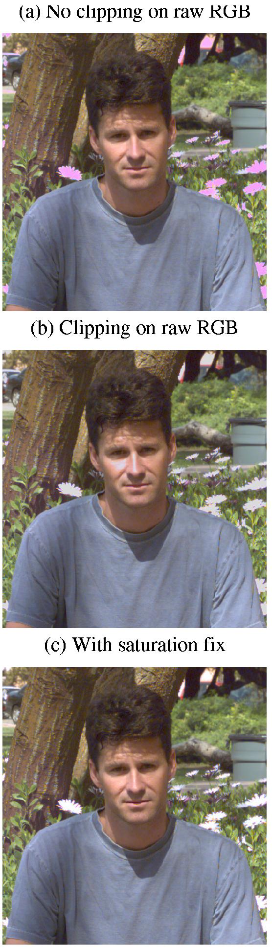
Another DCS200 image rendered without saturation fix (a), with pixel value clipping to a known white point (b), and with saturation fix (c).
To correct for the saturation, the image was first demosaiced using bilinear interpolation applied separately to each color channel. Prior distribution parameters were bootstrapped from non-saturated RGB values of the demosaiced image. We then applied the saturation fix algorithm. The algorithm was applied in order to the Green, Red, and Blue color channels. The results are shown in Fig. 3(c). With the saturation fix, the flowers' color appears considerably closer to its original white.
It is also of interest to look at the image when rendered using the white balance-clipping method, show in Fig. 3(b). In this case, the clipping method resulted in the correct (white) color of the flowers. However, because of the additional clipping performed on the red and blue channel, some of the large red values on the face region are clipped off, resulting in a false “highlight” near the nose region. In this case, our saturation fix algorithm improved the color of the flowers while kept the color on the face region intact, as compared to the clipping method.
Fig.4 shows another example. This image was captured on a Kodak DCS460 camera. The raw RGB image provided by DCS460 was in a non-linear 8-bit format, with a look-up table stored in the image header which allowed the pixel values to be converted back to linear RGB values. We performed this inverse lookup operation to obtain the linear raw RGB values used in our further processing. The original image had no saturated pixels. Since the image had high spatial resolution, we decided to create a high quality full color image by bilinearly demosaicing the original image and then reducing the image size by a factor of 4 on each dimension. This resulted in a 170 × 430 “true” image which had no saturation and few demosaicing artifacts. The gains of the 3 color planes were then adjusted digitally, and the pixel values clipped, to artificially create saturated pixels. This process allows us to examine how well the saturation fix algorithm recovers the true sensor values of a pixel in an image. In the artificially saturated image, 12% of the pixels have only the Red sensor saturated, and 0.4% of the pixels have both Red and Green sensors saturated. There were no saturated Blue sensors. The large number of saturated Red sensor values resulted in greatly under-estimated red values for some pixel locations, hence the un-natural greenish-blue highlights on the body of the car (Fig.4a). The Bayes saturation fix algorithm was applied to the saturated image, to the Red color plane first, then to the Green 20 color plane. When the white balance/clipping method was used (Fig.4b), the highlights on the car return to a more natural whitish color, but with under-estimated magnitude, resulting in an un-natural “faded paint” look, instead of the highlight look, especially on the roof of the car. In addition, the clipping produces a magenta artifact in the center of the car's windshield. After applying the saturation fix, the image appears much more realistic (Fig.4c).
Fig. 4.
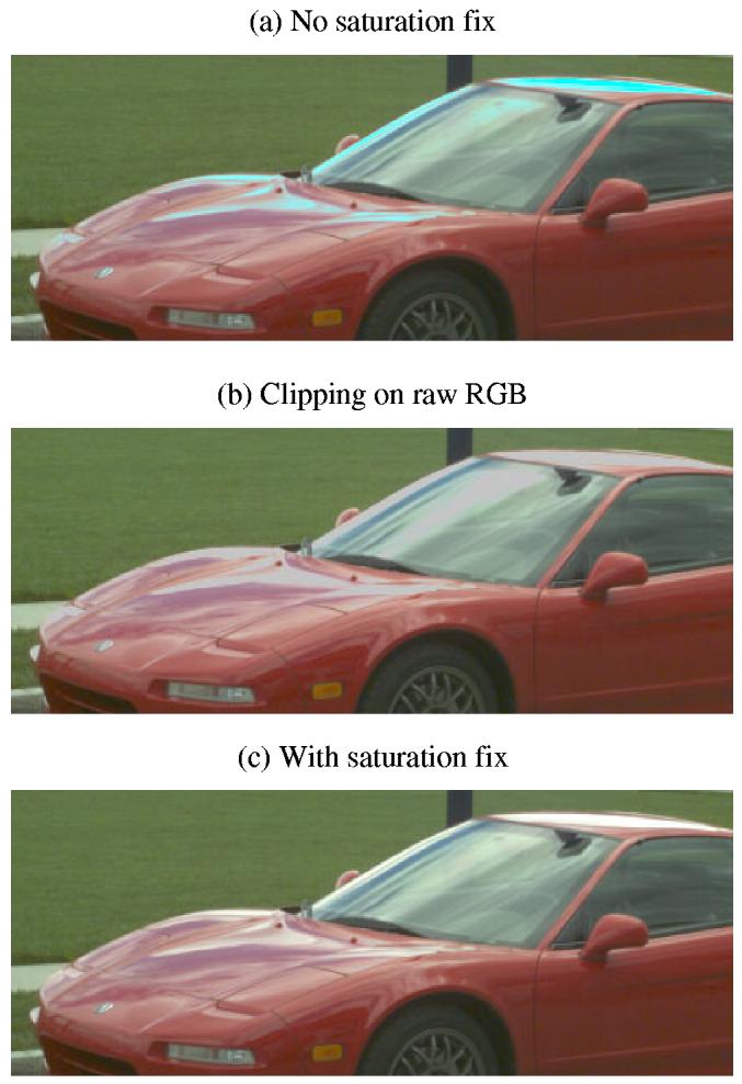
An image rendered without saturation fix (a), with pixel value clipping to a known white point (b), and with saturation fix (c). Saturated pixels were generated by adjusting gains and then clipping in the R and G color channels of an original image without any pixel saturation. This allows for comparison of the “true” values of the R and G pixels and the estimated values from our saturation fix algorithm.
Since we have the true pixel values for this image, we can compare these with those estimated by the saturation correction algorithm at saturated pixel locations. In Fig.5, estimated Red and Green color values are plotted against the true values before clipping was applied for all the pixels with sensor saturation. The estimated sensor values agree with the true sensor values at a coarse scale, with a systematic deviation for sensor values that are substantially larger than the saturation point. Even with the errors in the estimates, having the estimated values are better than using the saturated pixels at face value, as is shown in the rendered images in Fig.4.
Fig. 5.
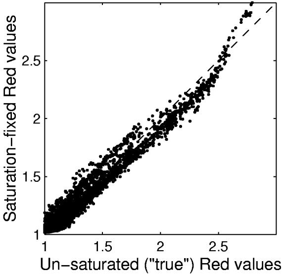
Comparison of true sensor values vs the saturated-and-fixed sensor values for the red car image in Fig.4. In the plot, a pixel value of 1 represent the saturation level.
Fig.1(c) shows the saturation fix applied to the truck image referred to in the introduction. Before the saturation fix, the white truck looks magenta due to the green sensor saturation. After the application of the fix, the white truck's color is corrected to be consistent with the areas without saturation. The algorithm was applied in order to the Green, Red, and Blue sensor values, as determined by the algorithm. In addition to removing the magenta color artifact, the shading on the hood of the car is recovered after the saturation fix, an improvement over the white balance-clipping method in Fig. 1(b).
We have tested our saturation fix algorithm on a number of other images, and in general, it performed well in fixing color errors in these images. The algorithm is particularly successful on images where the saturation occurs mostly in one color channel, where we have found it to be quite robust.
4. Summary and Discussion
We have presented a method for correcting the sensor values for saturated pixels in digital images. The method is based on the principles of Bayesian estimation, although its implementation incorporates some compromises to decrease computational complexity. Both simulations and application of the method to real image data indicate that the method is effective and that it can greatly improve the appearance of images. We close with a few comments about possible algorithm refinements and extensions.
A feature of our current analysis is that once the parameters of the prior are established, saturated pixels are corrected using only values from the other sensors at that location. It seems likely that additional information is carried by values at neighboring image locations and that using this information would improve algorithm performance. One approach would be to employ the same theoretical analysis we developed above, but to apply it to image data from a neighborhood of saturated pixels. In this approach, we would specify a prior for the joint distribution of pixels in (e.g.) N by N image blocks, and use the non-saturated pixel values within a block to correct saturated pixel values at the center of the block. The same formalism developed above still applies, but the dimensionality of the data increases. We6, 19 have previously used this approach develop a successful Bayesian demosaicing algorithm. Indeed, it is worth noting that fixing saturated pixels is a problem quite closely related to demosaicing. In the case of demosaicing, no information is available from the pixel value to be estimated, while for the case of fixing a saturated pixel we have a lower bound s for the true value. This suggests that future work might successfully combine demosaicing and adjustment of saturated pixels into a single step.
Another approach to including spatial information, which is much simpler to implement, is to estimate the parameters for the prior distribution from local regions of the image. For example, if a portion of a bright red car is saturated, it makes sense to estimate the covariance of the sensor values using non-saturated pixels that are spatially close to the saturation region and therefore likely to share the same color. For images with only a small number of saturated regions, this approach might also reduce the amount of calculation needed to estimate the prior covariance matrix.
Finally, we note that a different approach to dealing with saturated pixels is to avoid pixel saturation during image capture. As discussed in the introduction, this is not desirable for conventional (8- or 12-bit) sensors, since for avoiding any pixel saturation typically forces most of the image content to occupy a very small range of digital values. Indeed, the luminance range of natural scenes is often as high as 40000:1.27, 28 Some recently demonstrated imaging devices, however, are capble of capturing the full luminance range of many natural scenes.29, 30 Even for these devices, it may be that higher image quality is obtained by allowing a few pixels to saturate and correcting these with the algorithm presented here, as this exposure strategy will reduce the effect of quantization for most pixels in the image.
Acknowledgement
This work was partially supported by Hewlett Packard and Agilent Technologies. We also wish to thank Peter Delahunt and Jerome Tietz for providing some of the sample images used in this paper.
References
- 1.Longere P, Brainard DH. Simulation of digital camera images from hyperspectral input. In: van den Branden Lambrecht C, editor. Vision Models and Applications to Image and Video Processing. Kluwer Academic; Boston: 2001. pp. 123–150. [Google Scholar]
- 2.Holm J, Tastl I, Hanlon L, Hubel P. Color processing for digital photography. In: Green P, MacDonald L, editors. Colour Engineering: Achieving Device Independent Colour. John Wiley & Sons; 2002. pp. 179–217. [Google Scholar]
- 3.Holm J. A strategy for pictorial digital image processing; Proceedings of the IS&T/SID 4th Color Imaging Conference; 1996. pp. 194–201. [Google Scholar]
- 4.Kimmel R. Demosaicing: Image reconstruction from color CCD samples. IEEE Transactions on Image Processing. 1999;8:1221–1228. doi: 10.1109/83.784434. [DOI] [PubMed] [Google Scholar]
- 5.Kakarala R, Baharav Z. Adaptive demosaicing with the principal vector method. IEEE Transactions on Consumer Electronics. 2002;48:932–937. [Google Scholar]
- 6.Brainard DH, Sherman D. Reconstructing images from trichromatic samples: from basic research to practical applications; Proceedings of the 3rd IS&T/SID Color Imaging Conference; 1995. pp. 4–10. [Google Scholar]
- 7.Tao B, Tastl I, Cooper T, Blasgen M, Edwards E. Demosaicing using human visual properties and wavelet interpolation filtering; Proceedings of the IS&T/SID 7th Color Imaging Conference; 1999. pp. 252–256. [Google Scholar]
- 8.Viggiano JAS. Minimal-knowledge assumptions in digital still camera characterization I.: Uniform distribution, Toeplitz correlation; Proceedings of the IS&T/SID 9th Color Imaging Conference; 2001. pp. 332–336. [Google Scholar]
- 9.Brainard DH. Colorimetry. McGraw-Hill; New York: 1995. pp. 26.21–26.54. [Google Scholar]
- 10.Holm J. Photographic tone and colour reproduction goals. CIE Expert Symposium on Colour Standards for Image Technology. 1996:51–56. [Google Scholar]
- 11.Larson GW, Rushmeier H, Piatko C. A visibility matching tone reproduction operator for high dynamic range scenes. IEEE Transactions on Visualization and Computer Graphics. 1997;3:291–306. [Google Scholar]
- 12.Finlayson GD, Drew MS. The maximum ignorance assumption with positivity; Proceedings of the IS&T/SID 4th Color Imaging Conference; 1996. pp. 202–204. [Google Scholar]
- 13.Brainard DH, Freeman WT. Bayesian color constancy. Journal of the Optical Society of America A. 1997;14:1393–1411. doi: 10.1364/josaa.14.001393. [DOI] [PubMed] [Google Scholar]
- 14.Simoncelli EP. Bayesian denoising of visual images in the wavelet domain. In: Müller P, Vidakovic B, editors. Bayesian Inference in Wavelet Based Models. Springer-Verlag; New York: 1999. pp. 291–308. Lecture Notes in Statistics 141. [Google Scholar]
- 15.Weiss Y, Adelson EH. MIT; 1998. Slow and smooth: a Bayesian theory for the combination of local motion signals in human vision. A.I. Memo 1624, C.B.C.L. Paper No. 158. [Google Scholar]
- 16.Zhang X, Brainard DH. Method and apparatus for estimating true color values for saturated color values in digitally captured image data. US Patent No. 6731794 2004
- 17.Berger TO. Statistical Decision Theory and Bayesian Analysis. Springer-Verlag; New York: 1985. [Google Scholar]
- 18.Lee PM. Bayesian Statistics. Oxford University Press; London: 1989. [Google Scholar]
- 19.Brainard DH. Bayesian method for reconstructing color images from trichromatic samples. Proceedings of the IS&T 47th Annual Meeting. 1994:375–380. [Google Scholar]
- 20.Dillon WR, Goldstein M. Multivariate Analysis. John Wiley & Sons; New York: 1984. [Google Scholar]
- 21.Zhang X, Brainard DH. Bayes color correction method for non-colorimetric digital image sensors; IS&T/SID 12th Color Imaging Conference; 2004. Submitted to. [Google Scholar]
- 22.Adams JE, Jr., Hamilton JF., Jr. Adaptive color plane interpolation in single sensor color electronic camera. US Patent No. 5652621 1997
- 23.Trussell HJ, Hartwig RE. Mathematics for demosaicing. IEEE Transactions on Image Processing. 2002;11:485–492. doi: 10.1109/TIP.2002.999681. [DOI] [PubMed] [Google Scholar]
- 24.Vrhel MJ, Gershon R, Iwan LS. Measurement and analysis of object reflectance spectra. Color Research & Application. 1994;19:4–9. [Google Scholar]
- 25.Vora PL, Farrell JE, Tietz JD, Brainard DH. Image capture: modelling and calibration of sensor responses and their synthesis from multispectral images. IEEE Transaction on Image Processing. 2001;10:307–316. doi: 10.1109/83.902295. [DOI] [PubMed] [Google Scholar]
- 26.CIE . Bureau Central de la CIE; Vienna: 1995. Industrial Colour-Difference Evaluation. (Publication CIE 116-95). [Google Scholar]
- 27.Pattanaik S, Ferwerda J, Fairchild M, Greenberg D. A multiscale model of adaptation and spatial vision for realistic image display. Proceedings of SIGGRAPH'98. 1998:287–298. [Google Scholar]
- 28.Xiao F, DiCarlo JM, Catrysse PB, Wandell BA. High dynamic range imaging of natural scenes; Final Program and Proceedings of the 10th IS&T/SID Color Imaging Conference. Color Science, Systems and Applications; 2002. pp. 337–342. [Google Scholar]
- 29.Yang D, Fowler B. A 640×512 CMOS image sensor with ultrawide dynamic range floating-point pixel-level ADC. IEEE Journal of Solid State Circuits. 1999;34:1821–1834. [Google Scholar]
- 30.Nayar SK, Mitsunaga T. High dynamic range imaging: Spatially varying pixel exposures. Proceedings of IEEE CVPR. 2000 [Google Scholar]