Efficient Association Mapping of Quantitative Trait Loci with Selective Genotyping

Abstract

Selective genotyping (i.e., genotyping only those individuals with extreme phenotypes) can greatly improve the power to detect and map quantitative trait loci in genetic association studies. Because selection depends on the phenotype, the resulting data cannot be properly analyzed by standard statistical methods. We provide appropriate likelihoods for assessing the effects of genotypes and haplotypes on quantitative traits under selective-genotyping designs. We demonstrate that the likelihood-based methods are highly effective in identifying causal variants and are substantially more powerful than existing methods.

Mapping genes associated with quantitative traits is an important step toward genetic dissection of complex human diseases. Because the disease genes are unlikely to have very large effects on quantitative traits, power is a major concern in association studies, especially with the need to adjust for multiple testing. Despite the continuing improvements in genotyping efficiency, it is still highly expensive to genotype a large number of individuals, particularly in genomewide association studies. A cost-effective strategy is to preferentially genotype individuals whose trait values deviate from the population mean. Known as “selective genotyping,” this approach can result in a substantial increase in power (relative to random sampling with the same number of individuals), because much of the genetic information resides in individuals with extreme phenotypes.^1–7

Slatkin² suggested genotyping a selected sample of individuals with unusually high values of the quantitative trait, together with a random sample from the study population. Because selection depends on the phenotype, standard statistical methods that assume random sampling are not applicable. Slatkin² developed two tests: one comparing the allele frequencies between the selected sample and the random sample and one comparing the mean trait values among individuals with different genotypes in the selected sample. The two tests are approximately independent, so their P values can be combined to form an overall test. Slatkin² used simulation to show that his tests are more powerful than the simple t test (when the latter is applied to a random sample with the same number of individuals). Chen et al.⁵ recommended replacement of the random sample with a selected sample of individuals with unusually low trait values and described two sampling schemes to obtain the selected samples. They demonstrated through a simulation study that, with Slatkin’s three tests, their designs are more efficient than Slatkin’s original design.

In a recent Science report on obesity,⁸ one of the replication studies genotyped individuals from the 90th–97th percentile of the BMI distribution and those from the 5th–12th percentile, and another replication study genotyped individuals from the top and bottom quartiles. In both studies, the individuals with high and low BMI values were treated as cases and controls, respectively, and case-control methods (i.e., testing for allele-frequency differences between the two selected groups) were used for analysis.

Case-control methods disregard the actual trait values and are thus inefficient. Slatkin’s tests² do not make full use of the available data either—individuals who are homozygous for the minor allele are discarded, and the trait values in the random sample or the low-trait-value sample are not used at all. Recently, in this journal, Wallace et al.⁷ proposed a Hotelling’s T² test for normal traits, which they showed through simulation has increased power over Slatkin’s tests.² Wallace et al.’s test,⁷ which is essentially the standard t test in the case of a single marker, ignores the biased sampling nature of the selective-genotyping design and thus may not be optimal. Furthermore, none of the existing methods deals with haplotype-based testing or estimation of genetic effects.

In this report, we show how to properly and efficiently map QTLs with selective genotyping. We derive appropriate likelihoods that make full use of the available data and that properly reflect trait-dependent sampling. The corresponding inference procedures are valid and efficient. Our methods can be used to perform both genotype-based and haplotype-based association analyses. Their advantages over the existing methods are demonstrated through extensive simulation studies.

We consider two very general selective-genotyping designs. Under design 1, the quantitative trait is measured on a random sample of N individuals from the study population, and a subset of n individuals is selected for genotyping; the selection probabilities depend on the trait values. Under design 2, a random sample of n individuals whose trait values fall into certain regions is selected for genotyping, and the trait values are retained for only those individuals. Thus, the main difference between the two designs is that the trait values on those individuals who are not selected for genotyping are retained under design 1 but not under design 2. Under design 2, it is not necessary to specify N or to ascertain the individuals outside the selection regions.

Let Y_i be the trait value of the ith individual and G_i be the corresponding multilocus genotype denoting the number of minor alleles at each SNP site. The association between G_i and Y_i is characterized by the conditional density function P(Y_i|G_i;θ) indexed by a set of parameters θ. In the special case of a single locus with the additive mode of inheritance, P(Y_i|G_i;θ) may take the familiar form of the linear regression model

where ε_i is zero-mean normal with variance σ². In this case, θ=(α,β,σ²). Under the dominant (or recessive) mode of inheritance, G_i in equation (1) is replaced by the indicator of whether the ith individual has at least one minor allele (or, for the recessive model, two minor alleles). If there are multiple loci, then βG_i in equation (1) is replaced by an appropriate linear combination of individual genotype scores and (possibly) their cross-products. We denote the probability function of the genotype by P(G;γ), where γ represents the (multilocus) genotype frequencies.

Under design 1, the data consist of(Y_i,G_i)(i=1,…,n) and Y_i(i=n+1,…,N). (Without loss of generality, the data are arranged so that the first n records pertain to the n individuals who are selected for genotyping and the remaining (N-n) records to the unselected individuals.) The corresponding likelihood for θ and γ can be written as

where the summation over G is taken over all possible genotypes; a derivation is given in appendix A.

Under design 2, the data consist only of

which are a random sample from all the individuals whose trait values belong to a particular set 𝒞. We can use the likelihood for θ and γ,

or the likelihood for θ,

If only the individuals whose trait values are less than the lower threshold c_L or larger than the upper threshold c_U are selected for genotyping, then, under equation (1),

where Φ is the cumulative distribution function of the standard normal distribution.

We refer to expression (2) as the full likelihood and to equations (3) and (4) as the conditional likelihoods. These likelihoods properly reflect the selective-genotyping designs and use all the available data. Note that expression (2) is the same as the likelihood for a prospective study of size N in which genotype data are missing on N-n individuals. Under design 1, one may disregard the trait values of those individuals who are not selected for genotyping and use the conditional likelihoods, provided that the genotyped individuals are a random sample from set 𝒞. The maximum-likelihood estimators can be obtained by the standard Newton-Raphson algorithm. As shown in appendix A, the maximizations of equations (3) and (4) yield the same estimator of θ. By the likelihood theory, the maximum-likelihood estimators are approximately unbiased, normally distributed, and statistically efficient. Association testing can be performed by using the familiar likelihood-ratio, score, or Wald statistics.

The above description pertains to the analysis of genotype-phenotype association. It is also desirable to assess haplotype-phenotype association.^9–10 Let H_i denote the diplotype of the ith individual. The effects of haplotypes on the trait are characterized by the conditional density function P(Y_i|H_i;θ) indexed by a set of parameters θ. If we are interested in assessing the effect of a particular haplotype h^*, then P(Y_i|H_i;θ) may take the form

where Z(H_i) is the number of occurrences of h^* in H_i under the additive mode of inheritance, the indicator of whether H_i contains at least one h^* under the dominant mode of inheritance, and the indicator of whether H_i contains two copies of h^* under the recessive mode of inheritance. One may also define P(Y_i|H_i;θ) in such a way that multiple haplotypes are compared with a reference in a single model.⁹

Because haplotypes are not directly observed, it is necessary to impose some restrictions, such as Hardy-Weinberg equilibrium (HWE), on the diplotype distribution. For k=1,…,K, let h_k denote the kth possible haplotype in the population and let π_k denote the population frequency of h_k. Under HWE,

We denote the diplotype probability function by P(H_i;γ), where γ=(π₁,…,π_K).

Inference on haplotype effects must properly account for phase ambiguity. Note that

where 𝒮(G_i) is the set of diplotypes compatible with genotype G_i.⁹ Thus, the full likelihood and conditional likelihood analogous to expressions (2) and (3) are

and

where the second summation in expression (6) and the summation in the denominator of expression (7) are taken over all possible diplotypes. The maximizations of expressions (6) and (7) can be performed by the expectation-maximization (EM) algorithm or the Newton-Raphson algorithm; see appendix A. The maximum-likelihood estimators are approximately unbiased, normally distributed, and statistically efficient.

Note that β pertains to genetic effect in equation (1) and to haplotype effect in equation (5). If we are concerned with one SNP at a time, however, the models in equations (1) and (5) are the same. In that case, likelihoods of expressions (6) and (7) differ from expressions (2) and (3) in that the former impose HWE and allow missing genotype values, whereas the latter do not impose HWE and exclude subjects with missing genotype values. Thus, the former yield more efficient analyses, provided that HWE is a reasonable assumption.

We conducted extensive simulation studies to assess the performance of the proposed methods. We considered both designs 1 and 2. Specifically, we generated a random sample of N=5,000 individuals from the joint distribution of the trait value and genotype, and we identified the subset of all the individuals whose trait values are <c_L or >c_U. We then selected a random sample of n=500 individuals from that subset. By setting the genotypes of the unselected individuals to “missing,” we obtained the data under design 1; by deleting the unselected individuals altogether, we obtained the data under design 2. We evaluated both the full-likelihood and conditional-likelihood methods. These evaluations provided information about the relative efficiency of using full likelihood versus conditional likelihood under design 1 or, equivalently, the relative efficiency of design 1 versus design 2.

For comparison, we also evaluated the standard methods, which are based on the prospective likelihoods. For genotype-based analysis, the prospective likelihood⁷ is simply i=1nP(Y_i|G_i;θ); for haplotype-based analysis, the prospective likelihood is the first term in expression (6).¹⁰ In addition, we evaluated the case-control tests, which regard the upper and lower trait values as cases and controls, respectively.

In our first study, we generated the trait values from equation (1) with α=0, σ²=1, and β=0, 0.1, 0.2, 0.3, 0.4, and 0.5. We set (c_L,c_U) to (−0.5,0.5), (−1.0,1.0), (−1.5,0.5) or (−2.0,1.0). Under the condition that β=0, the thresholds of −2.0, −1.5, −1.0, −0.5, 0.5, and 1.0 correspond approximately to the 2nd, 7th, 16th, 31st, 69th, and 84th percentiles of the trait distribution, respectively. We considered three modes of inheritance—additive, dominant, and recessive—and various values of the minor-allele frequency (MAF). The genotypes were generated under HWE, and the analyses were performed both with and without this assumption. The results without the HWE assumption are summarized in table 1. The results with HWE are similar and thus omitted.

Table 1. .

Bias, SE, Average SEE, Coverage Probability of 95% CI (CP), and Power at the .05 Nominal Significance Level at a Candidate Locus Under Additive (A) and Dominant (D) Models with MAFs of .05 and Recessive (R) Model with MAF of .2^[Note]

		Full Likelihood					Conditional Likelihood					Prospective Likelihood
Model, β, and cL	cU	Bias	SE	SEE	CP	Power	Bias	SE	SEE	CP	Power	Bias	SE	SEE	CP	Power	CC Power
A:
0:
−.5	.5	.001	.12	.12	95.3	5.0	.001	.12	.12	95.2	5.0	.002	.18	.18	95.0	4.9	5.1
−1.0	1.0	.001	.09	.09	95.3	5.0	.001	.09	.09	95.3	5.0	.003	.23	.23	95.0	5.0	5.0
−1.5	.5	.009	.12	.12	95.4	5.1	.010	.12	.12	95.2	5.1	.001	.19	.19	95.0	4.9	4.5
−2.0	1.0	.014	.11	.11	95.8	5.3	.015	.12	.11	95.6	5.3	.002	.20	.20	95.2	4.8	5.0
.2:
−.5	.5	.001	.12	.12	95.0	40.9	.003	.12	.12	95.0	40.9	.111	.18	.18	91.1	40.6	34.7
−1.0	1.0	.003	.10	.10	95.0	59.0	.004	.10	.10	95.3	59.0	.291	.22	.23	75.6	58.6	55.0
−1.5	.5	.011	.13	.13	95.0	40.0	.014	.13	.13	94.8	40.0	.079	.15	.17	95.8	35.8	27.1
−2.0	1.0	.016	.13	.13	95.0	42.2	.020	.13	.13	94.9	42.2	.084	.14	.18	97.1	34.5	25.7
.3:
−.5	.5	.002	.12	.12	95.2	72.9	.004	.12	.12	95.5	73.0	.159	.17	.18	86.1	72.8	64.0
−1.0	1.0	.003	.10	.10	95.4	90.3	.004	.10	.10	95.3	90.2	.403	.20	.22	55.7	90.0	87.7
−1.5	.5	.010	.13	.13	94.6	70.7	.014	.14	.13	94.7	70.6	.084	.14	.17	96.2	66.5	51.7
−2.0	1.0	.016	.14	.14	94.7	75.2	.022	.14	.14	95.0	75.1	.076	.12	.17	98.5	68.6	55.2
D:
0:
−.5	.5	.001	.12	.12	95.3	5.0	.002	.12	.12	95.2	4.9	.002	.19	.19	95.1	4.9	5.1
−1.0	1.0	.001	.10	.10	95.3	5.0	.001	.10	.10	95.3	5.0	.003	.24	.24	95.1	4.9	4.9
−1.5	.5	.010	.12	.12	95.3	5.2	.010	.12	.12	95.1	5.2	.001	.20	.19	95.0	5.0	4.6
−2.0	1.0	.014	.12	.11	95.8	5.2	.015	.12	.12	95.6	5.2	.002	.21	.21	95.2	4.8	5.0
.2:
−.5	.5	.001	.12	.12	94.9	38.4	.003	.12	.12	94.9	38.5	.112	.19	.19	90.9	38.3	32.5
−1.0	1.0	.002	.10	.10	95.3	55.6	.003	.10	.10	95.3	55.6	.292	.23	.24	76.9	55.1	52.2
−1.5	.5	.009	.13	.13	95.2	36.8	.012	.13	.13	95.0	36.8	.080	.16	.18	95.6	33.2	26.2
−2.0	1.0	.016	.14	.13	94.9	40.1	.021	.14	.13	95.0	40.0	.090	.15	.18	96.9	32.9	24.7
.3:
−.5	.5	.002	.12	.12	94.7	69.9	.004	.12	.12	94.9	69.8	.162	.18	.19	86.3	69.7	60.9
−1.0	1.0	.004	.10	.10	95.2	88.2	.006	.10	.10	95.3	88.2	.417	.22	.23	56.3	88.0	85.0
−1.5	.5	.009	.14	.14	94.7	67.6	.013	.14	.14	94.7	67.5	.091	.15	.18	95.7	63.4	49.7
−2.0	1.0	.018	.14	.14	94.7	72.0	.024	.15	.14	95.1	72.0	.090	.13	.17	98.1	65.5	53.0
R:
0:
−.5	.5	−.001	.19	.19	95.3	5.4	−.001	.19	.19	95.3	5.4	−.002	.29	.29	94.7	5.2	4.8
−1.0	1.0	.005	.15	.15	95.9	4.9	.005	.15	.15	95.9	4.9	.011	.37	.37	95.2	4.7	5.0
−1.5	.5	.024	.20	.19	95.4	5.5	.026	.20	.19	95.4	5.5	−.000	.30	.30	94.9	5.1	4.8
−2.0	1.0	.041	.20	.19	96.0	5.4	.043	.20	.19	95.8	5.5	.004	.32	.32	95.5	4.5	4.7
.4:
−.5	.5	.005	.20	.19	94.5	58.1	.009	.20	.19	95.0	58.0	.201	.27	.28	90.2	57.3	48.9
−1.0	1.0	.018	.17	.16	95.5	79.0	.022	.17	.17	95.6	79.0	.524	.31	.35	67.9	78.2	73.9
−1.5	.5	.024	.22	.22	93.9	56.6	.031	.22	.22	94.4	56.5	.087	.20	.26	98.8	48.2	29.0
−2.0	1.0	.037	.23	.23	94.0	60.2	.048	.23	.23	94.2	60.1	.066	.17	.25	99.7	46.0	27.4
.5:
−.5	.5	.010	.20	.19	94.6	77.7	.014	.20	.20	95.2	77.7	.242	.26	.28	88.3	77.1	66.9
−1.0	1.0	.021	.17	.17	95.6	93.5	.026	.18	.17	95.6	93.4	.600	.28	.34	57.1	93.1	89.4
−1.5	.5	.018	.22	.22	94.2	74.9	.027	.22	.22	94.5	74.7	.068	.18	.25	99.2	68.0	45.1
−2.0	1.0	.027	.22	.23	94.1	79.0	.039	.23	.23	94.4	78.9	.027	.15	.24	99.8	68.0	46.7

Note.— Each entry is based on 10,000 simulated data sets. CC = case-control analysis.

Both the full and conditional likelihoods provide (virtually) unbiased estimators of genetic effects and correct type I error. The SE estimators (SEEs) accurately reflect the true variations, and the CIs have proper coverages. The conditional likelihood has nearly the same power as the full likelihood. As expected, the power is substantially higher under the additive and dominant models than under the recessive model (given the same MAF and the same effect size). The power increases as selection becomes more extreme. Also, the power tends to be higher when c_L and c_U are of the same distance from the population mean (as opposed to unequal distances), which implies that the optimal sample-size ratio between the upper and lower ends should be ∼1:1 (as in the case of the case-control design). In practice, the population mean may be unknown, or it may be easier to recruit subjects with high trait values than those with low trait values, or vice versa. Thus, it may not be feasible to set c_L and c_U the same distance from the population mean.

In the presence of a causal variant, both the estimator of the genetic effect and the SEE based on the prospective likelihood are biased upward, and the coverages of the CIs may be substantially below or above the desired levels. The prospective likelihood appears to preserve the type I error. The power of the prospective likelihood tends to be lower than that of the full and conditional likelihoods, especially when (c_L,c_U)=(-2,1) and under the recessive mode of inheritance. When (c_L,c_U)=(-2,1), the full and conditional likelihoods have power of ∼75% to detect effect size of 0.3 under the additive and dominant models with MAF=0.05, and they have power of ∼80% to detect effect size of 0.5 under the recessive model with MAF=0.2. By contrast, the prospective likelihood has <70% power in those two cases. Not surprisingly, the case-control tests, which disregard the actual trait values, are substantially less powerful than the proposed methods.

In the second study, we generated data in the same way as in the first study, but we performed the analysis at a marker locus that is in linkage disequilibrium (LD) with the potential causal SNP. The results are shown in table 2. The basic conclusions are the same as in the first study. As expected, the power is decreased when testing is performed at a marker locus rather than at the candidate locus.

Table 2. .

Type I Error and Power at a Marker Locus Linked to a QTL^[Note]

		Additive Model					Dominant Model					Recessive Model
cL	cU	β	Full	Cond	Pros	CC	β	Full	Cond	Pros	CC	β	Full	Cond	Pros	CC
−.5	.5	0	5.3	5.2	5.2	4.9	0	5.2	5.3	5.3	4.8	0	5.1	5.1	5.0	4.9
−1.0	1.0		5.2	5.2	5.1	4.8		5.2	5.2	5.2	4.7		5.7	5.7	5.6	4.8
−1.5	.5		4.7	4.6	4.7	5.2		4.5	4.5	4.7	5.2		5.4	5.4	5.0	5.2
−2.0	1.0		5.5	5.5	5.5	5.4		5.3	5.4	5.5	5.5		5.1	5.2	4.5	4.3
−.5	.5	.3	55.3	55.3	55.1	47.1	.3	51.9	51.8	51.6	44.1	.4	30.2	30.3	30.0	25.9
−1.0	1.0		76.0	76.0	75.8	71.0		72.7	72.7	72.3	67.9		45.0	45.0	44.4	41.2
−1.5	.5		54.0	54.0	49.9	39.0		49.9	50.0	46.3	37.4		29.5	29.4	24.5	14.2
−2.0	1.0		56.2	56.2	49.5	37.6		52.4	52.3	46.1	36.1		31.7	31.5	23.5	15.6
−.5	.5	.4	79.4	79.4	79.1	70.4	.4	75.6	75.7	75.5	67.0	.5	44.1	44.1	43.8	36.6
−1.0	1.0		93.7	93.7	93.5	91.2		92.0	92.0	91.8	88.7		63.3	63.3	62.6	56.9
−1.5	.5		75.8	75.7	72.5	55.4		72.6	72.7	69.7	53.8		42.0	41.8	36.5	20.9
−2.0	1.0		78.8	78.7	73.8	58.4		75.8	75.7	71.1	57.0		45.1	45.0	35.8	20.8

Note.— The MAFs of the QTL and marker locus are .05 and .06 under the additive and dominant models and are .2 and .25 under the recessive model. The standardized LD coefficient (D′) between the two loci is .9. Each entry is based on 10,000 simulated data sets. Full = full likelihood; Cond = conditional likelihood; Pros = prospective likelihood; CC = case-control analysis.

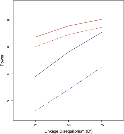
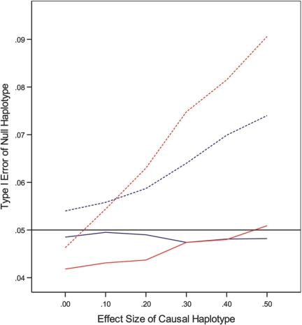
The third study was concerned with haplotype effects. We considered two SNPs with varying degrees of LD. The 11 haplotype—that is, the haplotype consisting of the minor allele at each site—had a potential effect on the trait value. We generated the trait values from equation (5) with α=0, σ²=1, and β=0, 0.1, 0.2, 0.3, 0.4, and 0.5. We considered three modes of inheritance: additive, dominant, and recessive. HWE was assumed in both the data generation and the analysis. We performed two types of analyses: the first analysis compared the 11 haplotype with the other three haplotypes, and the second analysis compared haplotypes 11, 10, and 01 with haplotype 00. Some of the testing results are displayed in figures 1 and 2.

Figure 1. .

Empirical power for detecting causal haplotype 11 at the nominal significance level of .05 under 2-SNP models with MAFs of .3 and .4 and with (c_L,c_U)=(-2,1) as a function of the LD. The solid and dotted red curves correspond to the conditional and prospective likelihoods, respectively, under the dominant model with β=.2, whereas the solid and dotted blue curves correspond to the conditional and prospective likelihoods, respectively, under the recessive model with β=.3.

Figure 2. .

Empirical type I error for testing null haplotype 10 at the nominal significance level of .05 under 2-SNP additive models with MAFs of .3 and .4 and D′ of .75 as a function of the effect size of causal haplotype 11. The solid and dotted red curves correspond to the conditional and prospective likelihoods, respectively, under (c_L,c_U)=(-2,1), whereas the solid and dotted blue curves correspond to the conditional and prospective likelihoods, respectively, under (c_L,c_U)=(-1,1). A solid black reference line is drawn at the nominal significance level of .05.

The full and conditional likelihoods provide (virtually) unbiased estimators of haplotype effects. The SEEs are very accurate, and the CIs have correct coverages. The two methods have proper control of the type I error and very similar power. Not surprisingly, the power increases as LD becomes higher and as selection becomes more extreme. The prospective likelihood yields biased estimation of haplotype effects and inappropriate CIs. As shown in figure 1, the prospective likelihood is less powerful than the full and conditional likelihoods, especially under a recessive mode of inheritance. Furthermore, the prospective likelihood yields inflated type I error for testing null haplotypes. The inflation of the type I error becomes more severe as the effect of the causal haplotype increases, as illustrated in figure 2. Again, the case-control methods⁹ are much less powerful than the proposed methods (data not shown).

The two designs considered in this report are quite general and flexible. Since the simulation studies indicated that conditional likelihoods are nearly as efficient as full likelihoods, one may simply adopt design 2 and retain the trait values for the genotyped individuals only. The choices of the selection thresholds do not require precise knowledge of the trait distribution, although the efficiency of the design will depend on which percentiles the thresholds correspond to. The likelihoods presented here can be easily modified to include a random sample, as in the original Slatkin design,² or to allow several selection regions with different sampling probabilities. Although we have focused on normally distributed traits, our methods can be applied to any trait distributions.

We focused on the analysis of a single marker or a small set of markers. Association studies typically involve many markers, so a large number of tests is performed. Adjustments for multiple testing can be made by permutation or Monte Carlo methods.¹¹

We can incorporate environmental covariates into the models and likelihoods of this report. In the presence of covariates, the likelihoods given in formulas (2), (3), (6), and (7) will involve the covariate distribution. The corresponding numerical algorithms are more complicated and will be presented elsewhere.

Appendix A

Derivation of Expression (2)

The data for design 1 can be written as (Y_i,R_i,R_iG_i)(i=1,…,N), where R_i indicates, by the values 1 versus 0, whether the ith individual is selected for genotyping. The likelihood function i=1NP(Y_i,R_i,R_iG_i) can be expressed as i=1NP(Y_i,R_i)P(R_iG_i|Y_i,R_i) or i=1NP(Y_i)P(R_i|Y_i)P(G_i|Y_i)^R_i, which is proportional to i=1NP(Y_i)P(G_i|Y_i)^R_i or i=1NP(Y_i,G_i)^R_iP(Y_i)^1-R_i, because the selection probabilities P(R_i|Y_i) are constants. This justifies expression (2).

Equivalence of Equations (3) and (4) in Estimating θ

It suffices to show that the profile likelihood for θ—that is, the maximum of expression (3) over γ for fixed θ—is equivalent to equation (4). By defining γ_g=P(G=g;γ), , and P_g(θ)=P(Y_i∈𝒞|G=g;θ), we can write the logarithm of expression (3) as . It then follows from simple algebraic manipulations that the profile log-likelihood for θ is , which is exactly the logarithm of equation (4), up to the constant .

EM Algorithm for Maximizing Expression (6)

We present an EM algorithm for the maximization of expression (6) by treating the H_i as missing data. The complete-data log-likelihood is

where I(·) is the indicator function. Define p_ikl=P[H_i=(h_k,h_l)|Y_i,G_i], where G_i is unknown for i=n+1,…,N. Then

where S(G_i) is the set of all possible diplotypes when G_i is unknown. In the E step of the EM algorithm, we evaluate the p_ikl at the current estimates of θ and γ. In the M step, we solve the equations

and

for θ and γ, respectively.

The linear regression model specifies that, conditional on H_i=(h_k,h_l), the quantitative trait Y_i is normally distributed with mean β^TZ(h_k,h_l) and variance σ², where Z(h_k,h_l) is a specific function of h_k and h_l and where β is the corresponding set of regression parameters. Note that Z(h_k,h_l) includes the unit component and that β corresponds to α and β of equation (5). If we are interested in comparing a particular haplotype h^* with all others, then Z(h_k,h_l)=[1,I(h_k=h^*)+I(h_l=h^*)]^T under the additive model, Z(h_k,h_l)=[1,I(h_k=h^*)+I(h_l=h^*)-I(h_k=h_l=h^*)]^T under the dominant model, and Z(h_k,h_l)=[1,I(h_k=h_l=h^*)]^T under the recessive model. In this case,

and the M step has explicit solutions

and

Newton-Raphson Algorithm for Maximizing Expression (7)

Under the linear regression model with thresholds c_L and c_U, expression (7) becomes

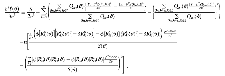
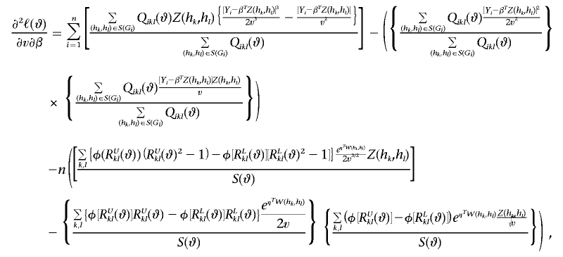
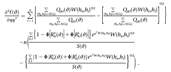
To incorporate the constraints that and π_k>0(k=1,…,K) into the calculations, we define π^*_k=π_k/π_K and η_k=logπ^*_k. For notational convenience, denote σ² as v. Let η=(η₁,…,η_K-1) and ϑ=(β,v,η). Then the log-likelihood is

where

Let

and

Also, let a^⊗2=aa^T, and let φ be the standard normal density function. Then

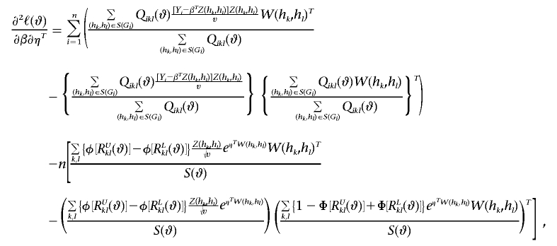and

References

- 1.Laitinen T, Kauppi P, Ignatius J, Ruotsalainen T, Daly MJ, Kääriäinen H, Kruglyak L, Laitinen H, de la Chapelle A, Lander ES, et al (1997) Genetic control of serum IgE levels and asthma: linkage and linkage disequilibrium studies in an isolated population. Hum Mol Genet 6:2069–2076 10.1093/hmg/6.12.2069 [DOI] [PubMed] [Google Scholar]
- 2.Slatkin M (1999) Disequilibrium mapping of a quantitative-trait locus in an expanding population. Am J Hum Genet 64:1765–1773 [DOI] [PMC free article] [PubMed] [Google Scholar]
- 3.van Gestel S, Houwing-Duistermaat JJ, Adolfsson R, van Duijn CM, van Broeckhoven C (2000) Power of selective genotyping in genetic association analyses of quantitative traits. Behav Genet 30:141–146 10.1023/A:1001907321955 [DOI] [PubMed] [Google Scholar]
- 4.Xiong M, Fan R, Jin L (2002) Linkage disequilibrium mapping of quantitative trait loci under truncation selection. Hum Hered 53:158–172 10.1159/000064978 [DOI] [PubMed] [Google Scholar]
- 5.Chen Z, Zheng G, Ghosh K, Li Z (2005) Linkage disequilibrium mapping of quantitative-trait loci by selective genotyping. Am J Hum Genet 77:661–669 [DOI] [PMC free article] [PubMed] [Google Scholar]
- 6.Cornish KM, Manly T, Savage R, Swanson J, Morisano D, Butler N, Grant C, Cross G, Bentley L, Hollis CP (2005) Association of the dopamine transporter (DAT1) 10/10-repeat genotype with ADHD symptoms and response inhibition in a general populations sample. Mol Psychiatry 10:686–698 10.1038/sj.mp.4001641 [DOI] [PubMed] [Google Scholar]
- 7.Wallace C, Chapman JM, Clayton DG (2006) Improved power offered by a score test for linkage disequilibrium mapping of quantitative-trait loci by selective genotyping. Am J Hum Genet 78:498–504 [DOI] [PMC free article] [PubMed] [Google Scholar]
- 8.Herbert A, Gerry NP, McQueen MB, Heid IM, Pfeufer A, Illig T, Wichmann HE, Meitinger T, Hunter D, Hu FB, et al (2006) A common genetic variant is associated with adult and childhood obesity. Science 312:279–283 10.1126/science.1124779 [DOI] [PubMed] [Google Scholar]
- 9.Lin DY, Zeng D, Millikan R (2005) Maximum likelihood estimation of haplotype effects and haplotype-environment interactions in association studies. Genet Epidemiol 29:299–312 10.1002/gepi.20098 [DOI] [PubMed] [Google Scholar]
- 10.Schaid DJ, Rowland CM, Tines DE, Jacobson RM, Poland GA (2002) Score tests for association between traits and haplotypes when linkage phase is ambiguous. Am J Hum Genet 70:425–434 [DOI] [PMC free article] [PubMed] [Google Scholar]
- 11.Lin DY (2005) An efficient Monte Carlo approach to assessing statistical significance in genomic studies. Bioinformatics 21:781–787 10.1093/bioinformatics/bti053 [DOI] [PubMed] [Google Scholar]