Linear Transformations and the k-Means Clustering Algorithm: Applications to Clustering Curves

Abstract

Functional data can be clustered by plugging estimated regression coefficients from individual curves into the k-means algorithm. Clustering results can differ depending on how the curves are fit to the data. Estimating curves using different sets of basis functions corresponds to different linear transformations of the data. k-means clustering is not invariant to linear transformations of the data. The optimal linear transformation for clustering will stretch the distribution so that the primary direction of variability aligns with actual differences in the clusters. It is shown that clustering the raw data will often give results similar to clustering regression coefficients obtained using an orthogonal design matrix. Clustering functional data using an L² metric on function space can be achieved by clustering a suitable linear transformation of the regression coefficients. An example where depressed individuals are treated with an antidepressant is used for illustration.

1 Introduction

Functional data applications, where each data point corresponds to a curve, have come to play a prominent role in statistical practice (e.g. Ramsay and Silverman, 1997, 2002). The curves in a functional data set often have a variety of distinctive shapes that can have important interpretations. Representative curve shapes can be found by clustering the curves (e.g. Heckman and Zamar, 2000; Abraham et al., 2003; James and Sugar, 2003; Luschgy and Pagés, 2002; Tarpey and Kinateder, 2003). The k-means clustering algorithm (e.g. Forgy, 1965; Hartigan and Wong, 1979; MacQueen, 1967) has been and remains one of the most popular tools for clustering data. When applied to functional data, k-means clustering results vary depending on how the curves are fit to the data. Ultimately, the problem of k-means clustering of functional data boils down to the behavior of the k-means algorithm for different linear transformations of the data which is the focus of this paper.

Let y₁(t), y₂(t), . . . , y_n(t) denote a sample of functional responses. In most applications the functions are only observed at a finite number of time points along with a random error. Thus, a regression model can be used to estimate the function:

$${\mathit{y}}_i=\mathit{X}{\mathit{b}}_i+{\mathit{∊}}_i,$$ (1)

where y_i = (y_i(t₁) + ∊_i1, y_i(t₂) + ∊_i2, . . . y_i(t_mi) + ∊_imi)′, ∊_i is a vector of random errors, b_i is the p × 1 vector of regression coefficients for the ith function and X is a design matrix determined by the choice of basis functions used to represent the functions (e.g. Ramsay and Silverman, 1997, Section 3.2). The estimated regression coefficients can be obtained using least-squares:

$${\widehat{\mathit{b}}}_i={({\mathit{X}}^{\prime }\mathit{X})}^{-1}{\mathit{X}}^{\prime }{\mathit{y}}_i.$$ (2)

A natural way to cluster the functions is to apply the k-means algorithm to the estimated regression coefficients ${\widehat{\mathit{b}}}_i$, i = 1, . . . , n.

Figure 1 shows fitted curves using a B-spline basis (de Boor, 1978) for n = 414 depressed subjects treated with Prozac for twelve weeks (McGrath et al., 2000). The functions are the estimated Hamilton Depression (HAM-D) responses as a function of time (scaled to take values between 0 and 1) for each subject where lower HAM-D scores correspond to lower levels of depression. The shapes of the curves are important indicators of the strength of placebo responses and drug responses for individual subjects. However, due to the large number of curves in Figure 1, it is difficult to pick out distinct and representative curve shapes.

Figure 1.

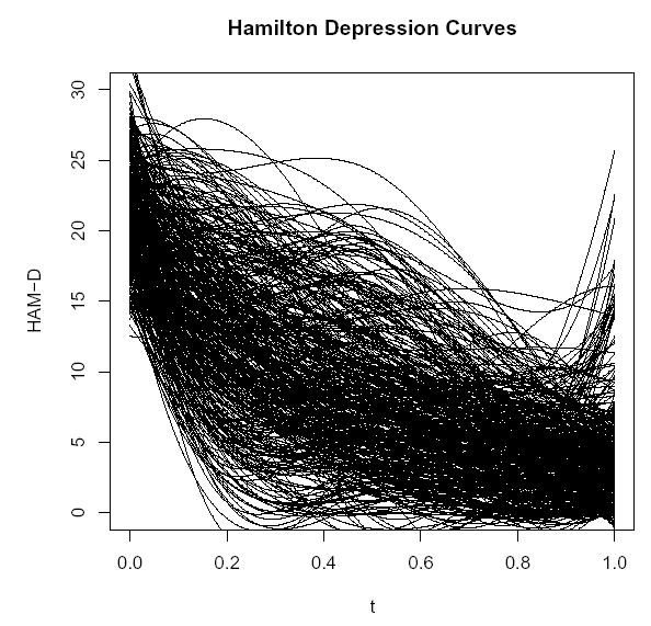
Estimated B-spline curves for HAM-D response over a 12 week period for n = 414 depressed subjects taking Prozac.

Figure 2 shows the k = 3 cluster mean curves obtained from the k-means algorithm for four different representations of this functional data. In panel A of Figure 2, the functional nature of the data is ignored and the raw data (the y_i’s) were plugged into the k-means algorithm. In panels B, C, and D, the estimated regression coefficients (2) using respectively a B-spline basis, a Fourier basis and a power basis (with an intercept and exponents −1, 1, 2, and 3) were clustered. For the power series basis in panel D, a functional L² metric was used in the k-means algorithm instead of the usual Euclidean metric (see Section 3). The B-spline representation used a single knot at t = 1/2 which was nearly optimal in terms of a cross-validation prediction error. The resulting design matrix for the B-spline basis was based on p = 5 cubic B-spline basis functions. Five basis functions were used for the Fourier and power series as well so that each basis representations corresponds to the same dimension reduction.

Figure 2.

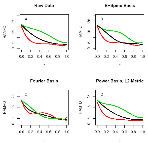
k = 3 cluster mean curves for the Prozac data from four different approaches: A. results from clustering the raw data y_i’s; B. results from clustering estimated B-spline coefficients; C: results from clustering estimated Fourier coefficients; D: results from clustering estimated coefficients from a power basis fit to the curves.

The results from clustering shown in panels A, B and D in Figure 2 are somewhat similar: (1) the lower curve corresponds to a very strong immediate improvement and then a leveling off indicating an initial placebo response before the drug has an effect; (2) the middle curve shows a steady improvement; (3) the top curve corresponds to subjects experiencing stronger improvement later in the trial, perhaps after the drug has had time to take effect. The cluster mean curves in panel C for the Fourier fits are considerably more bunched together and have different shapes. Incidently, the cluster results for the power basis are very similar to the Fourier results (panel C) if a Euclidean metric had been used instead of the L² metric.

Figure 2 highlights a very important point: The fitted curves for individual subjects using the B-spline, Fourier and power bases are almost identical and fit the data quite well but the cluster results for the different fits can differ considerably. The reason is because different methods of fitting curves correspond to different linear transformations of the raw data. Therefore the covariance structures for the regression coefficients differ causing the clustering results to differ as well. For instance, the first principal component of the estimated Fourier coefficient distribution accounts for 99.8% of the variability and consequently, the estimated cluster means from the Fourier fits lie approximately along the first principal component axis of the 5-dimensional coefficient space. The cluster means from clustering the B-spline coefficients on the other hand lie approximately in the 2-dimensional subspace spanned by the first two principal component axes (which explains only 51% and 28% of the variability respectively).

If A denotes an arbitrary square invertible matrix, the regression model (1) can be expressed as

$${\mathit{y}}_i=(\mathit{X}\mathit{A})({\mathit{A}}^{-1}{\mathit{b}}_i)+{\mathit{∊}}_i=\mathit{Z}{\mathit{a}}_i+{\mathit{∊}}_i,$$ (3)

where Z = XA and a_i = A⁻¹b_i. Although the fitted values from (1) and (3) are identical, k-means clustering of the ${\widehat{\mathit{b}}}_i$’s and the ${\widehat{\mathit{a}}}_i$’s generally yield different results. Standardized and weighted regression as well as fitting orthogonal polynomials use transformations similar to (3). It is well-known that results from the k-means algorithm depends on how the data is weighted (e.g. Milligan and Cooper, 1988; Gnanadesikan et al., 1995; Green et al., 1990; Milligan, 1989). The primary question of interest when clustering functional data is not necessarily how to choose individual weights, but more generally how best to linearly transform the data prior to clustering.

It is interesting to note that in the Prozac example above that clustering an appropriate linear transformation of the Fourier coefficients produces results almost identical to clustering the B-spline coefficients shown in panel B of Figure 2. The required linear transformation can be found by letting P_F = X_F (X′_F X_F)⁻¹ X′_F denote the “hat” matrix for projections onto the column space of X_F , the Fourier basis design matrix. Let ${\widehat{\mathit{X}}}_B={\mathit{P}}_F{\mathit{X}}_B$ denote the projection of the B-spline basis design matrix X_B onto the column space of X_F. Then using ${\widehat{\mathit{X}}}_B$ in place of X_B, the estimated B-spline coefficients ${\widehat{\mathit{b}}}_B$ can be approximated by

$$\begin{array}{l}{\widehat{\mathit{b}}}_B\approx {({\widehat{\mathit{X}}}_B^{\prime }{\widehat{\mathit{X}}}_B)}^{-1}{\widehat{\mathit{X}}}_B^{\prime }\mathit{y}={({\mathit{X}}_B^{\prime }{\mathit{P}}_F^{\prime }{\mathit{P}}_F{\mathit{X}}_B)}^{-1}{\mathit{X}}_B^{\prime }{\mathit{P}}_B\mathit{y}\\ ={({\mathit{X}}_B^{\prime }{\mathit{P}}_F{\mathit{X}}_B)}^{-1}{\mathit{X}}_B^{\prime }{\mathit{X}}_F{({\mathit{X}}_F^{\prime }{\mathit{X}}_F)}^{-1}{\mathit{X}}_F^{\prime }\mathit{y}\\ =\mathit{T}{\widehat{\mathit{b}}}_F\end{array}$$

where the transformation matrix T = (X′_BP_FX_B)⁻¹X′_BX_F, and ${\widehat{\mathit{b}}}_F$ equals the estimated coefficient vector using the Fourier design matrix. In the Prozac example, the cluster mean curves from clustering the transformed Fourier coefficients $\mathit{T}{\widehat{\mathit{b}}}_F$ are essentially indistinguishable from the cluster mean curves obtained by clustering the estimated B-spline coefficients shown in panel B of Figure 2. It should be noted that transformations of coefficients from one basis to approximate coefficients from another will not always produce nearly identical clustering results.

The remainder of the paper is organized as follows: Section 2 shows that clustering the raw data will often produce results very similar to clustering estimated regression coefficients from an orthogonal regression; Section 3 shows that the k-means algorithm using an L² function space metric is equivalent to clustering regression coefficients after an appropriate linear transformation; Section 4 discusses optimal linear transformations of the data for k-means clustering and provides a simple illustration for clustering linear functions. The paper is concluded in Section 5.

2 Clustering the Raw Data

In the Prozac example of Section 1, it turns out that clustering regression coefficients obtained using an orthogonal design matrix produces cluster mean curves that are essentially indistinguishable from those produced by clustering the raw data shown in panel A of Figure 2. That is, reducing the dimensionality of the data using the regression model appears to give no advantage over clustering the raw data. This section explains why.

First, certain linear transformations have no effect on k-means clustering. In particular, clustering p-dimensional observations, y_i’s, and the transformed data

$${\tilde{\mathit{y}}}_i=\mathit{\mu }+c\mathit{H}{\mathit{y}}_i$$ (4)

where μ ∈ ℜ^p, c ∈ ℜ¹, and H is an orthogonal p × p matrix, yield identical results. If ${\widehat{\mathit{\xi }}}_j,$ j = 1, . . . , k, are the cluster means found from clustering the ${\tilde{\mathit{y}}}_i$, then ${\mathit{H}}^{\prime }({\widehat{\mathit{\xi }}}_j-\mathit{\mu })/c$ are the cluster means from clustering the original data.

Let X = UDV′ denote the singular value decomposition of the design matrix X in (1). Then X_o = XVD⁻¹ = U is an orthogonal design matrix and b_o = DVb is the vector of associated regression coefficients. The least squares estimator of b_o is ${\widehat{\mathit{b}}}_o={({{\mathit{X}}^{\prime }}_o{\mathit{X}}_o)}^{-1}{{\mathit{X}}^{\prime }}_o\mathit{y}={\mathit{U}}^{\prime }(\mathit{U}{\mathit{b}}_o+\mathit{∊})={\mathit{b}}_o+{\mathit{U}}^{\prime }\mathit{∊}$. Define V to be a m × (m − p) matrix with orthonormal columns such that H = [U : V ] is an orthogonal m × m matrix. Since H′y is just a rotation of y, clustering the raw data will yield identical classifications as clustering H′y by (4). Now

$$\begin{array}{l}{\mathit{H}}^{\prime }\mathit{y}=\left(\begin{array}{c}{\mathit{U}}^{\prime }\hspace{0.17em}\mathit{y}\\ {\mathit{V}}^{\prime }\hspace{0.17em}\mathit{y}\end{array}\right)\\ =\left(\begin{array}{c}{\mathit{U}}^{\prime }(\mathit{U}{\mathit{b}}_o+\mathit{∊})\\ {\mathit{V}}^{\prime }\hspace{0.17em}(\mathit{U}{\mathit{b}}_o+\mathit{∊})\end{array}\right)\\ =\left(\begin{array}{c}{\widehat{\mathit{b}}}_o\\ {\mathit{V}}^{\prime }\hspace{0.17em}\mathit{∊}\end{array}\right).\end{array}$$

The raw data, after rotating by H′, has two orthogonal parts: the estimated orthogonal regression coefficients ${\widehat{\mathit{b}}}_o$ and a pure error part V′∊. Thus, if the error variance is zero, clustering the raw data is exactly equivalent to clustering the regression coefficients from an orthogonal design matrix. That is, both methods will produce identical clusters. Since the (rotated) raw data has a pure error component V′∊ that presumably contains no information on the true clusters, one would expect that clustering the estimated coefficients ${\widehat{\mathit{b}}}_o$ from an orthogonal design matrix to do a better job at recovering true clusters than clustering the raw data when the error variance is large. If the error variance is small relative to the variability of the regression coefficients, then clustering the raw data should yield essentially the same results as clustering estimated coefficients using an orthogonal design matrix which is what happens in the Prozac example of Section 1 when orthogonal design matrices are used.

3 Clustering Functional Data with an L² Metric

In standard applications of k-means clustering, data points in ℜ^p are assigned to clusters based minimal Euclidean distance to the cluster centers. If the data are functions, then an L² metric in function space may be a more appropriate metric to use for clustering. If y(t) is a functional observation and ξ(t) is a functional cluster mean, then the squared L² distance between these two functions on an interval [T₁, T₂] is

$$\parallel y-\xi {\parallel }^2={\int }_{T_1}^{T_2}{(y(t)-\xi (t))}^{2}dt.$$ (5)

Suppose functions y(t) are represented using a regression relation

$$y(t)={\beta }_0{u}_0(t)+{\beta }_1{u}_1(t)+\cdots +{\beta }_p{u}_p(t)+∊(t).$$

For instance, in a quadratic regression we would have u₀(t) = 1, u₁(t) = t, u₂(t) = t². Alternatively, the u_l(t) could be orthogonal polynomials or, in the case of a Fourier expansion, trigonometric functions. Denote the expansion of a cluster mean ξ(t) by $\xi (t)={\sum }_{l=0}^p{\gamma }_l{u}_l(t)$. The squared L² distance between a function y(t) and a cluster mean ξ(t) in (5) can be expressed as

$$\begin{array}{l}\parallel y-\xi {\parallel }^2={\int }_{T_1}^{T_2}{(y(t)-\xi (t))}^{2}dt\\ ={\int }_{T_1}^{T_2}\{\sum _{l=0}^p({\beta }_l-{\gamma }_l)u_l(t){\}}^{2}dt\\ =\sum _{l_1=0}^p\sum _{l_2=0}^p({\beta }_{l_1}-{\gamma }_{l_1})({\beta }_{l_2}-{\gamma }_{l_2}){\int }_{T_1}^{T_2}{u}_{l_1}(t)u_{l_2}(t)dt\\ =(\mathit{\beta }-\mathit{\gamma }{)}^{\prime }\mathit{W}(\mathit{\beta }-\mathit{\gamma })\\ =({\mathit{W}}^{1/2}(\mathit{\beta }-\mathit{\gamma }){)}^{\prime }({\mathit{W}}^{1/2}(\mathit{\beta }-\mathit{\gamma })),\end{array}$$

where β and γ are the vector of regression coefficients for y(t) and ξ(t) respectively, W is the symmetric (p + 1) × (p + 1) matrix with elements

$${\int }_{T_1}^{T_2}{u}_{l_1}(t)u_{l_2}(t)dt,$$ (6)

and W^1/2 is the symmetric square root of W. Thus, if one wishes to cluster functional data using an L² metric, then one can simply plug in the transformed regression coefficients W^1/2β into a standard k-means algorithm. This transformation was used in the Prozac example of Section 1 to obtain an L² metric clustering of the estimated power series basis coefficients (see panel D of Figure 2). As Tarpey and Kinateder (2003) noted, clustering regression coefficients is not appropriate if an L² metric is desired unless the functions u_l(t) are orthonormal over (T_1, T₂) in which case W = I and the L² metric in function space is equivalent to a Euclidean metric on the regression coefficients.

4 A Canonical Transformation for Clustering

The k-means algorithm may fail to find true clusters in a data set if there is substantial variability in the data unrelated to differences in clusters. In fact, there is nothing inherent in the k-means algorithm that guarantees that true clusters will be discovered. Instead the k-means algorithm tends to place sample cluster means where maximal variation occurs in the data. Thus, clustering functional data using the k-means algorithm will perform best if the linear transformations used to fit the curves stretch the data in a direction that corresponds to true cluster differences.

Basically the k-means algorithm begins with an initial set of k cluster means and then assigns individual data points to clusters depending on which cluster center the individual points are nearest. The cluster means are then updated based on the assignment of points to clusters and the algorithm continues to iterate until no more points are reassigned to clusters. Because the algorithm iterates by assigning points to the cluster whose center is closest, the optimization achieved by the algorithm is to find groupings that minimize the within group sum-of-squares, or equivalently, to maximize the between group sum-of-squares.

We will assume that differences between clusters lie in the random regression coefficients b in (1) and not in the random error ∊. Let μ_j and Ψ_j denote the mean and covariance matrix respectively of the random regression coefficient b for the jth cluster and let π_j denote the proportion of the population in cluster j = 1, 2, . . . , k. The covariance matrix for the b can be decomposed as

$$cov(\mathit{b})=\mathit{W}+\mathit{B},$$ (7)

where

$$\mathit{W}=\sum _{j=1}^k{\pi }_j{\mathbf{\Psi }}_j\hspace{0.17em}\text{and}\hspace{0.17em}\mathit{B}=\sum _{j=1}^k{\pi }_j({\mathit{\mu }}_j-\mathit{\mu })({\mathit{\mu }}_j-\mathit{\mu }{)}^{\prime },$$

are the within cluster and the between cluster covariance matrices respectively and where $\mathit{\mu }={\sum }_{j=1}^k{\pi }_j{\mathit{\mu }}_j.$ From (7) one can see that in order to optimize the k-means clustering, a transformation should be used that minimizes the contribution of the within cluster variability while maximizing the between cluster variability. A canonical discriminant function is defined as “linear combinations of variables that best separate the mean vectors of two or more groups of multivariate observations relative to the within-group variance” (Rencher, 1993). In canonical discriminant analysis, transformations based on vectors a_j that successively maximize (a′_jBa_j)/(a′_jWa_j) are used. The solution is to choose the a_j as the eigenvectors of W⁻¹B. A canonical transformation for clustering is now defined by first linearly transforming the regression coefficient vector into Fisher’s canonical variates followed by a stretching of the coefficient distribution to accent the between cluster variability and minimize the within cluster variability. In particular, consider a linear transformation that simultaneously diagonalizes W and B. Denote the spectral decomposition of W^−1/2BW^−1/2 by HDH′ where H is an orthogonal p × p matrix and W^1/2 is the symmetric square root of W. Let Γ = W^−1/2H. Assume the eigenvalues λ₁ ≥ λ₂ ≥ · · · ≥ λ_p in D are arranged from largest to smallest down the diagonal. Then from (7), the covariance matrix of Γ′b will be

$$\mathit{I}+\mathit{D}.$$ (8)

In order to accent the between cluster variability and diminish the contribution of the within cluster variability, one can further transform using a canonical transformation for clustering

$$\mathit{C}{\mathbf{\Gamma }}^{\prime }\mathit{b}$$ (9)

where C = diag(c_1, c₂, . . . , c_p) and the c_j ≥ 0 are appropriately chosen constants. From (8), the covariance matrix for the canonically transformed coefficients in (9) is C² + C²D. Thus, choosing large values of c_j corresponding to eigenvalues in D greater than one inflates the between cluster variability relative to the within cluster variability of the canonically transformed coefficients and setting c_j = 0 for eigenvalues between zero and one minimizes the contribution of the within cluster variability. For instance, suppose the cluster means lie on a line. Then multiplying the positive eigenvalue λ₁ in D by a large value of c₁ transforms the coefficient distribution by stretching it in the direction of the line containing the cluster means. Consequently, the k-means algorithm will place cluster means along this line for large values of c₁. If the cluster means lie approximately in a q-dimensional plane, then one would choose c₁, . . . , c_q to be large and the remaining c_j to be small. An interesting problem is to determine the optimal settings for the c_j in order to optimize the k-means algorithm according to minimizing a mean squared error or a classification error rate.

The canonical transformation of the regression coefficients in (9) can be adjusted for the random error in a regression model. Letting $\widehat{\mathit{b}}={({\mathit{X}}^{\prime }\mathit{X})}^{-1}{\mathit{X}}^{\prime }\mathit{y}$ denote the least-squares estimator of b, it follows from (1) that

$$cov(\widehat{\mathit{b}})=\mathit{W}+\mathit{B}+{\sigma }^2{({\mathit{X}}^{\prime }\mathit{X})}^{-1},$$ (10)

where σ² is the error variance and we have assumed the error components are independent. The canonical transformation for $\widehat{\mathit{b}}$ is the same as (9) except W is replaced by $\mathit{W}+{\widehat{\sigma }}^2{({\mathit{X}}^{\prime }\mathit{X})}^{-1}$. The following example illustrates the canonical transformation.

Example: An Simple Illustration of a Canonical Transformation

Consider k = 3 clusters of random linear functions y(t) = b₀ + b₁t + ∊. The y-intercepts and slopes were simulated from a three component normal mixture with mean values of y-intercept and slopes equal to (0, 1), (2, 1), and (3, 3) in the three clusters and a common within cluster covariance matrix equal to

$$\mathbf{\Psi }=\left(\begin{array}{cc}2& -1\\ -1& 6\end{array}\right).$$

The proportion of the population in each of the three clusters is taken to be π₁ = π₂ = π₃ = 1/3. The error variance is σ² = 0.25. Regression coefficients were estimated via least-squares. In addition, regression coefficient estimates were also estimated using an orthogonal design matrix X_o where X′_oX_o = I. Finally, a canonical transformation for clustering (9) was also used. If c₁ in C of (9) is too large relative to c₂, the sample cluster means from the k-means algorithm for the canonically transformed data will lie along a line which will not be optimal because the true cluster means defined above are not co-linear. Testing different values of c₁ with simulated data indicated that setting C = diag(3.5, 1) appears to be a nearly optimal canonical transformation in terms of minimizing the average squared difference between the estimated cluster means and the true cluster means. Figure 3 shows contours of equal density for the three cluster components with the horizontal axis corresponding to the y-intercept and the vertical axis corresponding to the slope. The top-left panel of Figure 3 shows the distribution for the original coefficient distribution; the coefficient distribution using the orthogonal design matrix is shown in the top-right panel; and the coefficients for the canonical transformation distribution is shown in the bottom panel.

Figure 3.

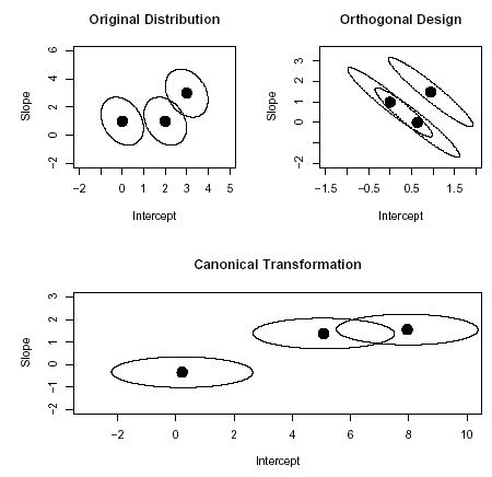
Contours of equal density for a k = 3 coefficient distribution. Top-left panel: the original distribution; Top-right panel: coefficient distribution using an orthogonal design matrix; Bottom panel: coefficient distribution using a canonical transformation.

In order to compare the performance of the three cases shown in Figure 3, 1000 data sets of size n = 100 were simulated for m_i = 10 equally spaced time points between t = 0 to 1. The k-means algorithm was run for each transformation using the R-software R Development Core Team (2003). The estimated cluster means for the orthogonal design matrix and the canonical coefficient distributions were transformed back to the original scale. For each simulated data set, a squared error was computed by summing the squared distances between each estimated cluster mean and the nearest true cluster mean. The squared error distributions, plotted in Figure 4, shows that clustering the original coefficients (without transforming) does very badly because the primary direction of within cluster variability is in a direction different than the between cluster variability. Clustering the coefficients from an orthogonal design matrix does much better in terms of the squared error because the transformation for the orthogonal design matrix provides more separation between clusters as shown in the top-right panel of Figure 3. The canonical transformation stretches the distributions in the direction with actual cluster differences and therefore performs the best in terms of squared error. With other parameter configurations, it is possible that clustering the original coefficients will perform better than clustering coefficients from an orthogonal design matrix.

Figure 4.

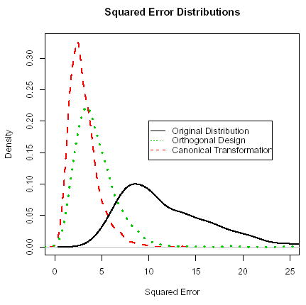
Density distributions for the squared error for clustering the estimated coefficients using (i) the original design matrix (solid curve), (ii) an orthogonal design matrix (dotted curve), and (iii) canonically transformed coefficients (dashed curve).

The main point of this section is that one should not blindly throw regression coefficients into a clustering algorithm and expect the results to coincide with actual clustering in the data. In particular, as the simulation example above illustrates, the performance of the k-means algorithm for clustering functional data can vary considerably depending how the functional data is transformed prior to clustering.

The optimal canonical transformation for clustering (9) requires knowing the true within and between covariance matrices which in practice are unknown. Unfortunately the sample between covariance matrix $\widehat{\mathit{B}}$ obtained from running the k-means algorithm will often reffect the major variability in the coefficient distribution regardless of whether or not this variability corresponds to true differences in cluster means. In the Prozac example of Section 1, the first eigenvector of the sample between covariance matrix $\widehat{\mathit{B}}$ for the Fourier coefficients is approximately equal to the first eigenvector of the Fourier coefficient covariance matrix, i.e. the k = 3 estimated cluster means from the k-means algorithm lie approximately on the first principal component axis.

In situations where cluster means lie in a common hyperplane, Bock (1987) proposes a projection pursuit clustering algorithm. This algorithm iterates by estimating the common hyperplane using the subspace spanned by the largest eigenvectors from the between group sums-of-squares-and-products matrix and then applying the k-means algorithm to the data projected onto this hyperplane. Bolton and Krzanowski (2003) note that Bock’s algorithm tends to find groups in the direction of the data corresponding to the largest variance and they propose a slightly different projection pursuit index to avoid this problem.

When actual cluster means do indeed lie along the major axis of variation (i.e. the first principal component), the k-means algorithm should perform quite well. This phenomenon occurs frequently in morphometric studies of growth and is called allometric extension (Hills, 1982; Bartoletti et al., 1999; Tarpey and Ivey, 2006). Let μ₁ and μ₂ denote the means of the two populations and suppose that the eigenvector associated with the largest eigenvalue of the covariance matrices in both populations is the same, call it β₁. Then the allometric extension model states that μ₂ − μ₁ = δβ₁ where δ is a constant (Flury, 1997, page 630). The allometric extension model may be reasonable in cases where two (or more) closely related species follow a common growth pattern where one species evolved to a larger overall size. If the first principal component accounts for a large proportion of the overall variance, then the k-means algorithm will tend to place estimated cluster means along the first principal component axis where the true cluster means reside. Thus, one would not want to automatically standardized the data before clustering in these cases because it may hurt the k-means algorithm ability to correctly determine groupings along the primary axis.

In a functional data analysis context, suppose the results of clustering curves produces roughly “parallel” cluster mean curves with the same shape. Parallel cluster mean curves occur quite often in practice when the variability in the intercepts of the curves overwhelms other modes of variation. In these cases, the first principal component variable will tend to coincide with the intercept approximately. Consequently all the cluster mean curves have basically the same shape as the overall mean curve and differ only in their intercepts. This is fine if the actual clusters differ in terms of their intercepts only. However, if curve shapes differ among groups, then the data needs to be transformed to minimize the variability of the intercept and allow the k-means algorithm to find distinct curve shapes. A couple possible solutions are to either drop the intercept term when clustering, or to cluster the derivatives of the estimated functions, see Tarpey and Kinateder (2003).

5 Discussion

An appealing aspect of functional data is that the observations are not just ordinary points in Euclidean space, but they are curves with distinct shapes. Clustering functional data is a useful way of determining representative curve shapes in a functional data set. However, the results from clustering curves depend on how the curves are fit to the data. The k-means clustering algorithm will perform best if the linear transformation used to fit the curves stretches the data in the direction corresponding to true cluster differences. Unfortunately optimal transformations required for clustering require knowing the true cluster means. A promising approach to solving this problem is to use projection pursuit clustering (Bolton and Krzanowski, 2003).

It has been assumed that the error in the regression model contained no information on the underlying clusters. This assumption may not always hold if the error variances in different clusters differ. In addition, if the wrong model is fit to the data producing non-random structure in the residuals, then this structure could contain information on clusters.

Clustering functional data by applying the k-means algorithm to the estimated coefficients is very easy and fast. There are two substantial disadvantages of the k-means algorithm: (i) the algorithm chops up the data into non-overlapping clusters, whereas in practice distinct groups in the data will often overlap; (ii) the k-means algorithm is completely nonparametric and does not take advantage of any valid parametric assumptions. Finite mixture models do not suffer from these two weaknesses and provide a useful alternative to the k-means algorithm. A simple approach is to plug the estimated coefficients into the EM algorithm for estimating parameters of a finite mixture. A computationally more complicated but highly flexible approach is to express the cluster/mixture model as a random effects model with a latent categorical variable for cluster membership and then estimate the parameters using maximum likelihood via the EM algorithm (James and Sugar, 2003; Muthén and Shedden, 1999).

References

- Abraham C, Cornillon PA, Matzner-Lober E, Molinari N. Scandinavian Journal of Statistics. 2003. Unsupervised curve clustering using b-splines; pp. 1–15. [Google Scholar]
- Bartoletti S, Flury B, Nel D. Allometric extension. Biometrika. 1999;55:1210–1214. doi: 10.1111/j.0006-341x.1999.01210.x. [DOI] [PubMed] [Google Scholar]
- Bock HH. On the interface between cluster analysis, principal component analysis, and multidimensional scaling. D. Reidel Publishing Company; 1987. pp. 17–34. [Google Scholar]
- Bolton RJ, Krzanowski WJ. Projection pursuit clustering for exploratory data analysis. Journal of Computational and Graphical Statistics. 2003;12:121– 142. [Google Scholar]
- de Boor C. A Practical Guide to Splines. Spinger-Verlag; New York: 1978. [Google Scholar]
- Flury B. A First Course in Multivariate Statistics. Springer; New York: 1997. [Google Scholar]
- Forgy EW. Cluster analysis of multivariate data: efficiency vs interpretability of classifications. Biometrics. 1965;21:768–769. [Google Scholar]
- Gnanadesikan R, Kettenring JR, Tsao SL. Weighting and selection of variables for cluster analysis. Journal of Classification. 1995;12:113–136. [Google Scholar]
- Green PE, Carmone RJ, Kim J. A preliminary study of optimal variable weighting in k-means clustering. Journal of Classification. 1990;7:271–285. [Google Scholar]
- Hartigan JA, Wong MA. A k-means clustering algorithm. Applied Statistics. 1979;28:100–108. [Google Scholar]
- Heckman NE, Zamar RH. Comparing the shapes of regression functions. Biometrika. 2000;87:135–144. [Google Scholar]
- Hills M. Allometry. In: Kotz S, Read CB, Banks DL, editors. Encyclopedia of Statistical Sciences. Vol. 1. Wiley; 1982. pp. 48–54. [Google Scholar]
- James G, Sugar C. Clustering for sparsely sampled functional data. Journal of the American Statistical Association. 2003;98:397–408. [Google Scholar]
- Luschgy H, Pagés G. Functional quantization of Gaussian processes. Journal of Functional Analysis. 2002;196:486–531. [Google Scholar]
- MacQueen J. Some methods for classification and analysis of multivariate observations. Proceedings 5th Berkeley Symposium on Mathematics, Statistics and Probability. 1967;3:281–297. [Google Scholar]
- McGrath PJ, Stewart JW, Petkova E, Quitkin FM, Amsterdam JD, Fawcett J, Reimherr FW, Rosenbaum JF, Beasley CM. Predictors of relapse during fluoxetine continuation or maintenance treatment for major depression. Journal of Clinical Psychiatry. 2000;61:518–524. doi: 10.4088/jcp.v61n0710. [DOI] [PubMed] [Google Scholar]
- Milligan G, Cooper M. A study of standardization of variables in cluster analysis. Journal of Classification. 1988;5:181–204. [Google Scholar]
- Milligan GW. A validation study of a variable weighting algorithm for cluster analysis. Journal of Classification. 1989;6:53–71. [Google Scholar]
- Muthén B, Shedden K. Finite mixture modeling with mixture outcomes using the EM algorithm. Biometrics. 1999;55:463–469. doi: 10.1111/j.0006-341x.1999.00463.x. [DOI] [PubMed] [Google Scholar]
- R Development Core Team. R: A language and environment for statistical computing. R Foundation for Statistical Computing; Vienna, Austria: 2003. ISBN 3-900051-00-3. [Google Scholar]
- Ramsay JO, Silverman BW. Functional Data Analysis. Springer: New York; 1997. [Google Scholar]
- Ramsay JO, Silverman BW. Applied Functional Data Analysis. Springer; New York: 2002. [Google Scholar]
- Rencher AC. Interpretation of canonical discriminant functions, canonical variates, and principal components. The American Statistician. 1993;46:217. [Google Scholar]
- Tarpey T, Ivey CT. Allometric extension for multivariate regression models. Journal of Data Science. 2006;4 [Google Scholar]
- Tarpey T, Kinateder KJ. Clustering functional data. Journal of Classification. 2003;20:93–114. [Google Scholar]