Optimizing the control of disease infestations at the landscape scale

Abstract

Using a contact-process model for the spread of crop disease over a regional scale, we examine the importance of the time scale for control with respect to the cost of the epidemic. The costs include the direct cost of treating infected sites as well as the indirect costs incurred through lost yield. We first use a mean-field approximation to derive analytical results for the optimal treatment regimes that minimize the total cost of the epidemic. We distinguish short- and long-term epidemics. and show that seasonal control (short time scale) requires extreme treatment, either treating all sites or none or switching between the two at some stage during the season. The optimal long-term strategy requires an intermediate level of control that results in near eradication of the disease. We also demonstrate the importance of incorporating economic constraints by deriving a critical relationship between the epidemiological and economic parameters that determine the qualitative nature of the optimal treatment strategy. The set of optimal strategies is summarized in a policy plot, which can be used to determine the nature of the optimal treatment regime given prior knowledge of the epidemiological and economic parameters. Finally, we test the robustness of the analytical results, derived from the mean-field approximation, on the spatially explicit contact process and demonstrate robustness to implementation errors and misestimation of crucial parameters.

There is increasing interest in the optimization of disease control at the landscape scale (1–5). This interest is motivated for crop and animal disease by the desire to reduce unnecessary use of pesticide and to minimize the cost of control relative to the costs of infection. Seeking an optimal strategy in this way opens up a rich suite of possibilities that range from treating all infected individuals, through treatment of a fixed or varying proportion of infected individuals, as circumstances change during the course of an epidemic, to no treatment at all. Finding the optimal strategy depends on the balance of economic and epidemiological parameters that reflect the nature of the host–pathogen system and the efficiency of control method. Progress therefore requires a combination of epidemiological and economic factors in modeling that hitherto have tended to remain separate.

Economic models have given insight into optimal control under constraints imposed by limited resources (6–8), but they frequently ignore the spatial and temporal dynamics of disease (9). Epidemiological modeling has largely focused on identifying the mechanisms responsible for epidemics (5, 10, 11) but has taken little account of economic constraints in analyzing control strategies. Recent exceptions include epidemiological models for the spread of severe acute respiratory syndrome (12, 13), foot and mouth disease (1, 2, 14–16), and avian flu (3), in which the efficiencies of different control strategies are compared, usually with respect to times for extinction of the invading pathogen. These models are often closely tied to the details of the specific host–pathogen system. Although these details are essential for the implementation of control, they sometimes obscure underlying principles of optimal disease control. A more generic approach applicable to a wide range of host–pathogen systems is given by Dybiec et al. (17), who showed how matching the scale of the control strategy with the natural scale of the epidemic spread can bring epidemics under control, even when there is long-distance, small-world dispersal, as well as local dispersal of the pathogen. Much epidemiological work is predicated on the assumption that an invading disease must be eliminated. For many plant, animal, and even human diseases, however, it is not axiomatic that elimination of the pathogen is economically viable, which refocuses attention on the relative costs and benefits of control and the effects of epidemiological parameters associated with disease transmission and efficiency of control on them (18–21). One natural way to approach the situation, which allows analytical progress for simple epidemiological models, is through variational calculus (22, 23). Control strategies are introduced into epidemiological models, and optimal strategies are derived by minimizing an objective function that incorporates costs of infection and control. Sethi and others (19, 24–29) have successfully examined a number of these models. Here, we use the approach of Sethi (21), which utilized Green's theorem to solve the optimization problem, and build on it to examine the trade-offs between epidemiological and economic parameters. We motivate the analysis for the control of disease spreading through an agricultural landscape, by using the contact process (30) to describe an epidemic propagating through a lattice of susceptible sites. This type of model can be used to describe the spread of disease in a fixed landscape, where each site represents a bounded subpopulation that the disease can inhabit, such as a field. The analyses are principally motivated for crop disease, in which a field, plantation, or sometimes a farm is the natural epidemiological unit for monitoring and controlling the spread of disease through the landscape. Thus for a given crop, such as wheat, a field is initially classified as susceptible (S). It becomes infected (more strictly infectious) (I), as it becomes capable of transmitting infection to neighboring fields. Treatment of an infected field by a fungicide speeds the rate of recovery of the field to the susceptible class, and hence the system is described by an SIS model (31). This form of transmission is typical of a wide range of diseases that spread predominantly over short distances so that spread occurs between neighboring fields. The model applies to many soil-borne and splash-dispersed fungal pathogens and to viral pathogens vectored by short-range movement of aphid and other invertebrate vectors. By keeping the model generic, in this way the results also hold for simplified models of animal diseases, where the epidemiological unit is the herd, flock or, again, an entire farm.

We show how the optimal control strategies depend on the balance between economic and epidemiological parameters as well as the initial density of infected units (e.g., fields) in the population. Specifically, we ask the following questions. Is the conventional strategy associated with the contact process optimal, whereby a fixed proportion of infected fields is treated? If not, what is optimal and why? We give particular attention to the importance of the time frame over which control is envisaged and how it affects the optimal strategy. A distinction is made between a short period, typically a single season, and a long time frame, extending over many seasons that would be typical of a perennial crop or of disease in natural environments. Analysis of strategies over a long term necessarily involves a discount rate to account for alternative investment of resources for control, whereas that for a single season arguably does not (23). We first derive analytical solutions from a mean-field approximation of the contact process, from which to identify optimal control strategies. These strategies are nonspatial; that is, they do not rely on any knowledge of the location of disease in the landscape. The advantage of such strategies is that they are less susceptible to implementation errors arising from cryptic infection, in which infectious sites remain nonsymptomatic for a period (18), than are strategies that track the explicit location of infections in the landscape. From these nonspatial strategies we derive policy plots that serve to identify optimal strategies, given some knowledge of the epidemiological and economic parameters and the current level of infestation. We then run extensive numerical simulations to test that these strategies are also optimal (among the set of all nonspatial strategies) for the spatially explicit contact process and therefore provide a link between the mean-field analysis and the motivational example (the spatial spread of disease). Finally, we consider the robustness of the strategies to implementation errors and misestimation of crucial parameters, and the advantages and limitations of this approach for the control of disease in the agricultural landscape are discussed.

The Model.

In a contact process, each site of a lattice exists in one of two states, healthy or infected. Infected sites pass disease on to healthy neighbors and recover at a given rate, whereupon they become immediately susceptible to reinfection (SIS). Because a susceptible site must have an infected neighbor to become infected, the disease-free state is absorbing; persistence of the epidemic depends on the transmission rate and the recovery rate. By treating the occupancy of each site as statistically independent and assuming spatial homogeneity, we can derive a mean-field approximation for the proportion of infected sites (ρ) given by

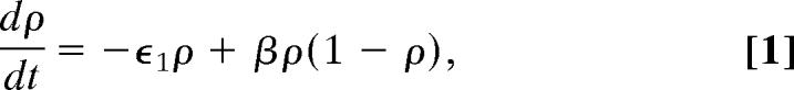where ϵ₁⁻¹ is the infectious period of each site and β the transmission rate, which is essentially an aggregated parameter composed of the transmission rate between pairs of infected and susceptible sites and the coordination number that describes the contact structure between infected and susceptible sites (30, 32).

The application of control to a given site may be assumed to reduce the infectious period leading to increased recovery rates from ϵ₁ to ϵ₂, of that site to the susceptible state. By applying control randomly to k of the n possible sites in the landscape we derive the state equation with control k ∈ [0, n], given by,

This equation implies that there exists a critical level of treatment k = k_c given by

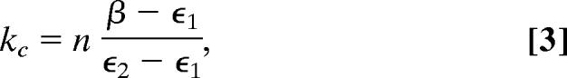such that if k > k_c the disease will be eradicated in the long term. The existence of the phase transition is ensured by imposing the conditions ϵ₁ < β and ϵ₂ ≥ β. Note that although it is convenient to express the phase transition in terms of k_c because it maps onto control strategies as envisaged here, the phase transition could also be expressed in terms of the familiar epidemiological concept of the basic reproductive number, R₀ (10), by a simple transformation of Eq. 2 whereby R₀ = βn/[(n − k)ϵ₁ + kϵ₂]. Thus, the condition k > k_c is equivalent to R₀ < 1, the widely used epidemiological criterion for the prevention of disease invasion. The existence of a phase transition has also been proven for the contact process (33, 34). However, the critical parameter values at which the phase transition takes place differ from the mean-field case because of the effect of spatial structure. Approximations of the critical values have been provided by using simulations (35) and series analysis (36–39) for lattices with low dimensionality.

Optimal Control.

The objective is to control the number of sites receiving treatment [k = k(t)] such that the total cost of infection and treatment is minimized over time. Under the assumption that the cost of treatment is linearly related to the amount administered, and similarly for the cost of infection (21, 29), the cost functions for short and long time scales are given, respectively, by

where c is the cost per infected site per unit of time, d is the cost per treated site per unit of time, r is the discount rate, and T is the length of the season. The discount rate represents the rate the policymaker is willing to pay to trade off the value of treatment today against the ensuing cost of increased infection in the future (23). By using the Pontryagin maximum principle [supporting information (SI) Appendix A], the optimal solution for both the long and short time scale problems is given by

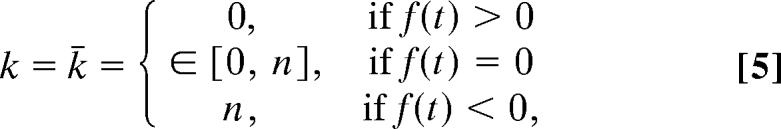where f(t) = ψρ(ϵ₂ − ϵ₁) + d and ψ is the costate variable (or shadow price of infection). The costate variable is governed by the differential equation

Treatments applied to all or no sites (k = n or k = 0) are termed extreme solutions, and intermediate coverage is termed a singular (or interior) solution. The costate variable indicates the marginal benefit of reducing the stock of infection. Because infection is harmful, it is always negative. A change Δk in the level of treatment causes the density of infected sites to change by −^Δk/_nρ(ϵ₂ − ϵ₁), and therefore the social value of this change is −ψ^Δk/_nρ(ϵ₂ − ϵ₁). The total cost of achieving such an outcome is d^Δk/_n. When treatment coverage is intermediate, so that variation in either direction is possible, the marginal cost of changing the coverage must be exactly equal to the social benefit. Thus, we obtain −ρψ(ϵ₂ − ϵ₁) = d, which is the condition f(t) = 0 for an interior (or singular) solution in Eq. 5. If the marginal cost of changing the coverage is different from the benefit received from the resulting change in infection, extreme coverage should be adopted. For example, if the cost of increasing coverage is less than the associated benefits, complete coverage (k = n) should be adopted, which is equivalent to the condition −ρψ(ϵ₂ − ϵ₁) > d, or f(t) < 0 in Eq. 5 (40). The behavior of the function f(t) dictates the nature of the optimal strategy. It is permissible to have solutions contained within the limits of treatment (singular solutions) only if f(t) = 0 for some nonzero length of time. Otherwise, the solution contains only the extreme levels of treatment, which is termed a “bang-bang” solution. A bang-bang solution may contain any number of switches from one extreme to the other over the course of the epidemic.

Results

The key difference between optimal short- and long-term disease control is the existence of a singular solution. It can be shown analytically (SI Appendix B) that singular solutions are not possible in the short time scale problem unless β/(ϵ₂ − ϵ₁) = c/d. This strict and exact condition is unlikely to be satisfied in natural systems, and so it can effectively be ruled out as a realistic option for policy decisions. Therefore, the optimal treatment regime involves extreme policies only, either treating all of the sites or none of them. Hence, the critical value k_c can be ruled out as a candidate. It can also be demonstrated analytically that if β/(ϵ₂ − ϵ₁) < c/d, then the optimal strategy is to treat all sites initially and then switch to no treatment at some determinable time (SI Appendix B). Otherwise, it is optimal not to treat at all.

For long-term control, the singular solution exists and is given by

As in the case of short-term control, the qualitative nature of the optimal control strategy can be derived entirely analytically by analysis of the phase space (SI Appendix C and SI Fig. 4). There are three possibilities for the optimal path, which are summarized in a policy plot (Fig. 1a and SI Fig. 4). The optimal strategy is determined by a relationship that relates the economic and epidemiological parameters and also depends on the prevalence of the infection when treatment is first administered. There exists a critical relation such that when c/d < β/(ϵ₂ − ϵ₁), the optimal strategy is to treat no sites at all, but when c/d > β/(ϵ₂ − ϵ₁), the optimal strategy changes radically to a two-phase strategy that begins with treating all (or no) sites (depending on the initial density of infection) and then switches to the interior level of treatment. The optimal time to switch is when the density of infection reaches the equilibrium value corresponding to k = k* (Fig. 1a). As the cost per infection increases relative to the cost per treated site, the optimal long-term level of infection approaches zero as the singular solution k* asymptotes to k_c. Fig. 2 shows some illustrative examples of optimal long- and short-term treatment regimes and the corresponding paths of infection.

Fig. 1.

Policy plots. (a) Mean-field model. (b) Contact process. Given that the initial density of infection is known, and we have an estimate of the epidemiological and economic parameters, we can use the policy plot as a tool to obtain the qualitative nature of the optimal treatment regime. The arrows indicate the progression toward the steady state for each strategy. In b, the dots represent the optimal equilibrium levels of infection for high, medium, and low initial infection densities. They vary because different epidemic realizations were used in each case. The three parameters are given in Table 1 and were used in both deterministic and spatially explicit cases.

Fig. 2.

Optimal treatment strategies and infection paths. (a and c) Long time frame case. (b and d) Short time horizon case. The critical level of treatment (k_c), derived from the mean-field model, is shown for comparison (dashed line) in all panels.

Numerical Testing and Sensitivity.

With the qualitative nature of the optimal treatment strategies for the mean-field model established, we now revert to the original contact-process formulation to test these strategies. The optimal strategies developed by using the mean-field formulation are independent of space. They are effective, and arguably achievable strategies that are easily implemented in practice (providing we have an estimate of the disease parameters) because they do not rely on any detailed knowledge of the location of disease in the landscape. When we test these strategies on the contact process, we are not testing for absolute optimality over all strategies (because absolute optimality is sure to depend on a knowledge of spatial location of infection). We are testing for optimality over all nonspatial strategies; that is, strategies that do not rely on any knowledge of the location of disease (as in the mean-field case). Given that the mean-field approximation has the same qualitative properties as the explicitly spatial system, we use spatial simulation to test the hypothesis that the optimal treatment regimes also share the same qualitative properties. We also test the sensitivity of the strategies to implementation errors and misestimation of crucial parameters.

Scaling the parameters from the mean-field to the spatially explicit is not straightforward (41–43). The transmission rate in the mean-field case (β) is assumed to be the rate at which an individual susceptible site becomes infected by an infected neighbor, multiplied by the number of possible contacts in the neighborhood (four in this case) (32). In reality, the transmission rate depends on the number of neighboring sites, which is dynamically changing in time. For this reason, we cannot simply map the optimal strategies derived from the mean-field model onto the spatially explicit case. Instead, we concern ourselves with demonstrating that the qualitative nature of the optimal strategy in the mean-field case (Fig. 1a) is the same as in the contact process. We ran replicated simulations to find the optimal nonspatial strategy among all possible constant and single-switch strategies. These simulations were performed over three initial levels of infection (ρ₀ low, medium, and high) and multiple cost ratios (c/d) (Fig. 1b). The optimal long-term level of infection was plotted for each initial level of infection (dots in Fig. 1b) and averaged (dashed line). The policy plots derived analytically from the mean-field model and numerically from the contact process are qualitatively identical but quantitatively different. The quantitative differences, such as the level of treatment required to maintain a given level of infection [which is significantly lower in the spatially explicit case because of the short-range spread (ref. 30)], derive from the effects of spatial structure.

The major implementation error in the case of long-term control is likely to be in the estimation of critical epidemiological parameters (such as the transmission rate), which could lead to a deflection of the boundaries among strategies in the policy plot. We examine this scenario for the case in which the recommended strategy involves a switch from treating all sites to treating k* sites once infection reaches a critical level. We perform this examination for a range of values of k around k* to simulate misjudgment of the values for the critical level of infection associated with misestimation of epidemiological parameters. We also compare this result with various constant strategies (for fixed k) because they represent the most practical alternatives to the switching strategy (Fig. 3a). The optimal strategy (when k* is estimated correctly) does not perform significantly better than the best constant strategy (in this case where treatment is held at 55% coverage). The true worth of the two-phase approach is in its robustness to misestimation of k*. It is apparent that undertreating in the constant strategy case could lead to significant loss, whereas the two-phase approach is remarkably robust against underestimating k* (Fig. 3a).

Fig. 3.

Testing the robustness of the optimal strategies by using spatial simulations. (a) Total discounted cost of an epidemic vs. the estimated value of k*. Two strategies are compared, a constant strategy where treatment remains at the estimated level of k* throughout, and the two-phase strategy of switching from maximum treatment to k*. Note that the epidemic runs with epidemiological parameters β and ϵ_i fixed at the correct values, so incorrect estimation of k* results from not knowing these values. (b) Cost of an epidemic (relative to the most cost-effective constant strategy, which was determined numerically to be ≈55% treatment) vs. the time of the switch (relative to the length of the season) from maximum to zero treatment. In both the short and long time frame cases, there were 50 realizations for each parameter set, with the default parameter values given in Table 1.

Over a single season, the optimal treatment strategy is simply to treat all sites and then switch off treatment at some critical point before the end of the season (providing the cost ratio is above a given critical value). Testing this strategy against the range of single-switch and constant strategies for a range of parameter variations (as performed in the long time frame case) demonstrated that the qualitative nature of the optimal strategy is identical in the mean-field and contact-process formulations.

The only difficulty in implementing this strategy is in finding the optimal time to switch, which cannot be derived analytically. Simulations reveal that if the optimal switch time is missed, then the switching policy does not always outperform the constant strategy (Fig. 3b). However, there is significant margin for error if optimality is not achieved. The best constant strategy was the strategy of treating approximately 55% of sites for the entire season, and it was determined numerically a posteriori. Varying the parameter values yielded similar outcomes.

Discussion

Using a mean-field, SIS model derived from the contact process we have rigorously derived the optimal treatment strategies that minimize the total cost of an epidemic over short and long time scales. The mean-field exhibits a bifurcation in stability of the nonzero equilibrium point as the level of treatment changes. This qualitative property is shared with the spatial lattice formulation. The goals were to examine the relationship between the optimal treatment strategy and the critical level of treatment required to eradicate the disease and to investigate how the time scale of control affects this relationship. Although the system studied is a simple representation of the spread of crop disease in a static landscape, it demonstrates the importance of economic considerations in epidemiological studies (28, 44) and allows us to extract some general principles that can then be tested in more realistic models for specific host–pathogen combinations.

The analyses give rise to recommendations for optimal strategies that differ from current conventions, where, for many diseases of annual and perennial crop plants, all infected fields are routinely treated. It is clear that simple analysis of epidemiological models would suggest that complete treatment of infected fields is not necessary if the objective is to prevent invasion of disease through the landscape or to prevent persistence (5, 45). Here the default for a system approximated by the contact process is to treat a proportion of fields, given for the mean-field approximation by k_c (Eq. 3), but doing so ignores the economic constraints associated with the cost of infection and the cost of treatment. Combining the two by using variational calculus (22) demonstrates that the epidemiological strategy is not necessarily optimal and leads to a set of alternative strategies, the outcome of which depends on the time frame of interest. The set of alternative strategies reflects, of course, the inclusion or otherwise of a discount rate (23) in the objective function, to be minimized. Here we have equated short-term regimes with a single season, for which we exclude the discount rate, comparing them with discounted longer-term regimes extending over multiple seasons. Note that it is the discount rate that separates the short- and long-term strategies, so the long time frame problem could just as easily be formulated as a finite time problem over more than one season (by replacing ∞ in Eq. 4 by large T). The results, in each case, depend on the relationships between the trade-offs in transmission and recovery rates for the epidemiological parameters and the ratio of costs for infection and treatment in the economic parameters (Figs. 1 and 2). Although both regimes can give rise to a singular solution, the criterion involving matching of the trade-offs in epidemiological with economic parameters is so exact for the short time horizon that we reject it as a plausible strategy. Doing so leaves only a bang-bang solution for the short time horizon provided [β/(ϵ₂ − ϵ₁)] < (c/d). The singular solution holds, however, for the long time horizon (Fig. 1), with treatment of a fixed proportion (k = k*) of infected fields, where k* < k_c. In this case, the optimal strategy is a switch from an extreme level of treatment to a level comparable with the critical level required for pathogen extinction. Over a shorter time scale, it becomes nonoptimal to treat near criticality, and instead it is best to switch between extreme treatments. This result is an intuitive one because the pathogen dynamics over a long time scale will eventually settle to equilibrium, whereas over short time scales, such as within a single growing season, the system will often remain in a transient state. Our model does not take account of the effect of interrupted transients associated with a long time scale for successive seasons of annual crops. Here, transients are routinely interrupted by harvesting, with successive epidemics being initiated by inoculum carried over from previous crops or by invasion from more distant sites for overwintering (4). The discontinuities remove the possibility of analytical results, but these systems are amenable to numerical investigation.

The relationship between the epidemiological and economic parameters determines a critical point at which a radically different strategy becomes optimal and is summarized for the long time frame case by a policy plot (Fig. 1a). The policy plot can be used to determine the nature of the optimal treatment regime, given prior knowledge of the epidemiological and economic parameters. The analytic results obtained from the mean-field formulation were tested on the spatially explicit contact-process model by using numerical simulation (Fig. 1b) and were found to be qualitatively identical but quantitatively different (because of the effects of spatial structure). It is important to note that the derived strategies are nonspatial. The advantage of nonspatial strategies is that they do not depend on a knowledge of the spatial location of disease. The strategies derived for the deterministic model outperformed the traditional constant policy and were shown to be robust against implementation errors. The robustness of the deterministic strategies was especially true in the case of long-term treatment, where misestimation of the interior level of treatment k* had little effect on the overall cost of the epidemic.

Previous authors have found optimal singular solutions for epidemiological models with bifurcations. Both Sethi (21) and Goldman et al. (19) considered SIS models, whereas Barrett (28) analyzed a static economic model with bifurcation and a Nash equilibrium. The analyses presented here go beyond these models in analyzing the trade-off between the epidemiological and economic parameters for different time scales and in testing the robustness of the strategies in a spatially explicit scheme.

We made certain assumptions to simplify the optimization, such as a linear relationship between the cost and the amount of treatment and infection. If this relationship were not the case, it would lead to a more complicated optimal strategy that would dynamically change in time and hence would not be as practical or manageable. We also assumed that treatment has no lasting effect. This assumption will not change the qualitative nature of the optimal path but may alter the timings of the switches between phases of treatment. The contact process is itself a crude approximation for the spread of disease through the landscape, in that it treats the infectious status of individual fields as a binary process and assumes that the transmission is restricted to neighboring fields arranged on a lattice. Simple extensions of the model are possible, notably to introduce structured metapopulations in which allowance is made for the build-up of infection within fields before transmission to other fields (11), to allow for off-lattice or lattice with gap distribution of susceptible sites and to the inclusion of explicit dispersal kernels for the longer distance dispersal of pathogens between infected and susceptible sites.

Methods

Although the optimal strategy for the long time frame problem is derived entirely analytically, numerical methods were used to determine the time of the switch for the optimal strategy within the short time horizon. Doing so involved a deterministic analysis of alternative switching times.

Contact-process simulations were performed on a lattice consisting of n = 10,000 sites (two-dimensional square lattice 100 × 100 with periodic boundary conditions). The default parameters used in the simulations are given in Table 1. The results hold for a wide range of initial densities and parameter values. The system was updated in a synchronous way until it reached steady state and the cost integral (J_∞) converged. Spread was possible in the von Neumann neighborhood (nearest neighbor spread) of each site. Treatment on a site increases the probability of recovery at the next update but has no lasting effect. To obtain the optimal constant strategy (i.e., the optimal strategy from the set of strategies that treat the same number of sites at each time step), we used a simple binary search algorithm.

Table 1.

Default parameters used in simulations

Symbol	Meaning	Default value
ρ0	Initial infected density	0.1
n	Population size	10,000
β	Transmission rate	0.1
ϵ1	Natural recovery rate	0.01
ϵ2	Recovery rate with treatment	0.11
c	Cost per infected site per unit time	2
d	Cost per treated site per unit time	1
r	Discount rate	0.01

The values given here are used in numerical simulations unless stated otherwise, although the qualitative results presented in this work held for any parameter realizations.

To obtain the policy plot (Fig. 1b), tests were performed on a smaller lattice (50 × 50) because of the computation time for each simulation, but isolated cases were tested on the larger lattice. We tested all possible constant strategies as well as single-switch strategies between all possible interior levels of treatment, which was done by using a single epidemic realization and then repeated on a second realization. In the vast majority of cases, the strategy that minimized the cost was the same in both cases (and is plotted in Fig. 1b). Very occasionally, two qualitatively different strategies were derived from each realization, leading to additional realizations to determine the likely optimal. Realizations were performed for three initial levels of infection (ρ₀ = 0.1, 0.3, and 0.5). For each initial level of infection, the optimal strategy was derived over a range of cost ratios (c/d) and the optimal long-term level of infection recorded (as dots in Fig. 1b) varied slightly because different epidemic realizations were used in each case. Further tests revealed that alternative parameter values resulted in qualitatively identical policy plots.

Abbreviation

SIS model

susceptible-infected-susceptible to reinfection model.

References

- 1.Ferguson NM, Donnelly CA, Anderson RM. Science. 2001;292:1155–1160. doi: 10.1126/science.1061020. [DOI] [PubMed] [Google Scholar]
- 2.Tildesley MJ, Savill NJ, Shaw DJ, Deardon R, Brooks SP, Woolhouse MEJ, Keeling MJ. Nature. 2006;440:83–86. doi: 10.1038/nature04324. [DOI] [PubMed] [Google Scholar]
- 3.Ferguson NM, Cummings DAT, Cauchemez S, Fraser C, Riley S, Meeyai1A, Iamsirithaworn S, Burke DS. Nature. 2005;437:209–214. doi: 10.1038/nature04017. [DOI] [PubMed] [Google Scholar]
- 4.Stacey AJ, Truscott JE, Asher MJC, Gilligan CA. Phytopathology. 2004;94:209–215. doi: 10.1094/PHYTO.2004.94.2.209. [DOI] [PubMed] [Google Scholar]
- 5.Gilligan CA. Adv Bot Res. 2002;38:1–64. [Google Scholar]
- 6.Lee PY, Matchar DB, Clements DA, Huber J, Hamilton JD, Peterson ED. Ann Intern Med. 2002;137:225–231. doi: 10.7326/0003-4819-137-4-200208200-00005. [DOI] [PubMed] [Google Scholar]
- 7.Trotter CL, Edmunds WJ. BMJ. 2002;324:1–6. doi: 10.1136/bmj.324.7341.809. [DOI] [PMC free article] [PubMed] [Google Scholar]
- 8.Worrall E, Rietveld A, Delacollette C. Am J Trop Med Hyg. 2004;71:136–140. [PubMed] [Google Scholar]
- 9.Gilligan CA. In: Battling Resistance to Antibiotics and Pesticides: An Economic Approach. Laxminarayan R, editor. Washington, DC: Resources for the Future; 2003. pp. 221–243. [Google Scholar]
- 10.Anderson RM, May RM. Phil Trans R Soc London B. 1986;314:533–568. doi: 10.1098/rstb.1986.0072. [DOI] [PubMed] [Google Scholar]
- 11.Park AW, Gubbins S, Gilligan CA. Oikos. 2001;94:162–174. [Google Scholar]
- 12.Lipsitch M, Cohen T, Cooper B, Robins JM, Ma S, James L, Gopalakrishna G, Chew SK, Tan CC, Samore MH, et al. Science. 2003;300:1966–1970. doi: 10.1126/science.1086616. [DOI] [PMC free article] [PubMed] [Google Scholar]
- 13.Riley S, Fraser C, Donnelly CA, Ghani AC, Abu-Raddad LJ, Hedley AJ, Leung GM, Ho L, Lam T, Thach TQ, et al. Science. 2003;300:1961–1966. doi: 10.1126/science.1086478. [DOI] [PubMed] [Google Scholar]
- 14.Keeling MJ, Woolhouse MEJ, Shaw DJ, Matthews L, Chase-Topping M, Haydon DT, Cornell SJ, Kappey J, Wilesmith J, Grenfell BT. Science. 2001;294:813–817. doi: 10.1126/science.1065973. [DOI] [PubMed] [Google Scholar]
- 15.Keeling MJ, Woolhouse MEJ, May RM, Davies G, Grenfell BT. Nature. 2003;421:135–142. doi: 10.1038/nature01343. [DOI] [PubMed] [Google Scholar]
- 16.Ferguson NM, Donnelly CA, Anderson RM. Nature. 2001;413:542–548. doi: 10.1038/35097116. [DOI] [PubMed] [Google Scholar]
- 17.Dybiec B, Kleczkowski A, Gilligan CA. Phys Rev Ser E. 2004;70 doi: 10.1103/PhysRevE.70.066145. 066145. [DOI] [PubMed] [Google Scholar]
- 18.Dybiec B, Kleczkowski A, Gilligan CA. Acta Phys Pol B. 2005;36:1509–1526. [Google Scholar]
- 19.Goldman SM, Lightwood J. Topics in Economic Analysis and Policy. Vol 2. Berkeley, CA: Berkeley Electronic Press; 2002. pp. 1–24. [Google Scholar]
- 20.Gupta NK, Rink RE. Math Biosci. 1973;18:383–396. [Google Scholar]
- 21.Sethi S. Biometrics. 1974;30:681–691. [PubMed] [Google Scholar]
- 22.Pinch E. Optimal Control and the Calculus of Variations. London: Oxford Univ Press; 1993. [Google Scholar]
- 23.Dixit AK, Pindyck RS. Investment Under Uncertainty. Princeton: Princeton Univ Press; 1994. [Google Scholar]
- 24.Sethi S. J Optim Theory Appl. 1978;29:615–627. [Google Scholar]
- 25.Sethi S. J Opl Res Soc. 1978;29:265–268. [Google Scholar]
- 26.Sethi SP, Thompson GL. INFOR 19. 1981;4:279–291. [Google Scholar]
- 27.Greenhalgh D. Math Biosci. 1987;88:125–158. [Google Scholar]
- 28.Barrett S. J Eur Econom Assoc. 2003;1:591–600. [Google Scholar]
- 29.Rowthorn R. In: Optimal Treatment of Disease Under a Budget Constraint. Halvorsen R, Layton DF, editors. Cheltenham, UK: Edward Elar; 2004. pp. 20–35. [Google Scholar]
- 30.Marro J, Dickman R. Nonequilibrium Phase Transitions in Lattice Models. Cambridge, UK: Cambridge Univ Press; 1999. [Google Scholar]
- 31.Murray JD. Mathematical Biology. I. An Introduction. 3rd Ed. Berlin: Springer; 2002. [Google Scholar]
- 32.Joo J, Lebowitz JL. Phys Rev E. 2004;69 066105. [Google Scholar]
- 33.Liggett TM. Interacting Particle Systems. New York: Springer; 1985. [Google Scholar]
- 34.Durrett R. Lecture Notes on Particle Systems and Percolation. New York: Springer; 1985. [Google Scholar]
- 35.Grassberger P, de laTorre A. Ann Phys. 1979;122:373–396. [Google Scholar]
- 36.Brower RC, Furman MA, Moshe M. Phys Lett B. 1978;76:213–219. [Google Scholar]
- 37.Dickman R. Phys Rev B. 1989;40:7005–7010. doi: 10.1103/physrevb.40.7005. [DOI] [PubMed] [Google Scholar]
- 38.Dickman R, Jensen I. Phys Rev Lett. 1991;67:2391–2394. doi: 10.1103/PhysRevLett.67.2391. [DOI] [PubMed] [Google Scholar]
- 39.Jensen I, Dickman R. Phys Rev E. 1993;48:1710–1725. doi: 10.1103/physreve.48.1710. [DOI] [PubMed] [Google Scholar]
- 40.Rowthorn R, Brown GM. In: Battling Resistance to Antibiotics and Pesticides: An Economic Approach. Laxminarayan R, editor. Washington, DC: Resources for the Future; 2003. pp. 42–62. [Google Scholar]
- 41.Keeling MJ, Grenfell BT. J Theor Biol. 2000;203:51–61. doi: 10.1006/jtbi.1999.1064. [DOI] [PubMed] [Google Scholar]
- 42.Green DM, Kiss IZ, Kao RR. J Theor Biol. 2006;239:289–297. doi: 10.1016/j.jtbi.2005.07.018. [DOI] [PubMed] [Google Scholar]
- 43.Keeling MJ, Eames TD. J R Soc Interface. 2005;2:295–307. doi: 10.1098/rsif.2005.0051. [DOI] [PMC free article] [PubMed] [Google Scholar]
- 44.Geoffard P-Y, Philipson T. Am Econ Rev. 1997;87:222–230. [Google Scholar]
- 45.Anderson RM, May RM. Infectious Disease of Humans: Dynamics and Control. Oxford: Oxford Science Publications; 1991. [Google Scholar]
Associated Data
This section collects any data citations, data availability statements, or supplementary materials included in this article.