Spatial localization accuracy of radiologists in free-response studies: inferring perceptual FROC curves from mark-rating data

Abstract

Free-response data consists of a set of mark-ratings pairs. Prior to analysis the data is classified or “scored” into lesion and non-lesion localizations. The scoring is done by choosing an acceptance-radius and classifying marks within the acceptance-radius of lesion centers as lesion localizations, and all other marks are classified as non-lesion localizations. The scored data is plotted as a free-response receiver operating characteristic (FROC) curve, essentially a plot of appropriately normalized numbers of lesion localizations vs. non-lesion localizations. Scored FROC curves are frequently used to compare imaging systems and computer aided detection (CAD) algorithms. However, the choice of acceptance-radius is arbitrary. This makes it difficult to compare curves from different studies and to estimate true performance. To resolve this issue the concept of two types of marks is introduced: perceptual hits and perceptual misses. A perceptual hit is a mark made in response to the observer seeing the lesion. A perceptual miss is a mark made in response to the observer seeing a (lesion-like) non-lesion. A method of estimating the most probable numbers of perceptual hits and misses is described. This allows one to plot a perceptual FROC operating point and by extension a perceptual FROC curve. Unlike a scored FROC operating point, a perceptual point is independent of the choice of acceptance-radius. The method does not allow one to identify individual marks as perceptual hits or misses – only the most probable numbers. It is based on a 3-parameter statistical model of the spatial distributions of perceptual hits and misses relative to lesion centers. The method has been applied to an observer dataset in which mammographers, and residents with different levels of experience were asked to locate lesions in mammograms. The perceptual operating points suggest superior performance for the mammographers and equivalent performance for residents in the first and second mammography rotations. These results and the model validation are preliminary as they are based on a small dataset. The significance of this study is showing that it is possible to probabilistically determine if a mark resulted from seeing a lesion or a nonlesion. Using the method developed in this study one could perform acceptance- radius independent estimation of observer performance.

1. INTRODUCTION

The free-response receiver operating characteristic (FROC) paradigm (1-6) is being increasingly used in the assessment of medical imaging systems (7, 8), particularly in the evaluation of computer aided detection (CAD) (9-11) algorithms. The paradigm differs from the traditional receiver operating characteristic (ROC) method (12-14) in that it seeks location information from the observer, rewarding the observer when the reported disease is marked in the appropriate location, and penalizing the observer when it is not. This task is more relevant to the clinical practice of radiology where it is not only important to identify disease, but also to offer further guidance regarding other characteristics (such as location) of the disease. In the FROC paradigm the data-unit is a mark-rating pair where a variable number (0, 1, 2,…) of mark-rating pairs can occur on an image. A mark is the indicated location of a region that was considered worthy of reporting (i.e., sufficiently suspicious) by the radiologist. The rating is a number representing the degree of suspicion, or confidence level, that the region in question is actually a lesion. In the ROC paradigm the data-unit is a single rating per image and no location information is collected. Several methods of analyzing free-response data have been described (6, 9-11, 15, 16). All of these methods share a well-known weakness that is detailed below.

Before FROC data can be analyzed it needs to be scored. Scoring refers to the investigator's decision to classify each mark either as a lesion-localization (LL) or as a nonlesion-localization (NL). [In order to avoid confusion with ROC studies we avoid use of the terms “true positives” or “false positives” to describe the classification of marks.] The classification into LL or NL is done by adopting a closeness or proximity criterion. Intuitively, if a mark is close to a lesion then it ought to be classified as a LL and conversely if it is far from any lesions it ought to be classified as a NL. However, what constitutes “close” is at the discretion of the investigator. In the past, researchers have used varying criteria to decide if a mark is close enough to be classified as a LL (17-19). For example, any mark made within the boundary of a lesion could be considered a LL (8). Another possibility is to select a distance criterion, termed acceptance-radius by us (6), and if a mark falls within this distance of the center of a lesion then it is classified as a LL and all other marks are classified as NLs. The choice of the acceptance-radius has an obvious effect on the observer's performance. Choosing a larger acceptance-radius will increase the number of marks that are scored as LLs and decrease the number of NLs thereby increasing apparent FROC observer performance. This work addresses the issue of how to resolve the arbitrariness of the choice of the acceptance-radius and its effect on performance measurement.

A brief review of FROC curves (2) follows. Assume that one arbitrarily chooses a value of the acceptance-radius and scores the marks into LLs and NLs. Associated with each mark is a numerical rating. Assume that the ratings are continuous and that a large number of images are used in the study so that sampling effects are absent and a continuous curve can be realized. A typical FROC curve for a moderate choice of acceptance-radius (AR) is shown in Fig. 1, labeled “AR = medium”. A point on the FROC curve is defined by selecting a cutoff ζ and counting only marks with ratings exceeding this value. The ordinate y(ζ) of this point is the number of lesion-localizations divided by the total number of lesions. The abscissa x(ζ) is the number of non-lesion localizations divided by the number of images. The FROC curve is the plot of y(ζ) vs. x(ζ) as ζ is varied. As ζ decreases from ∞ to −∞, y(ζ) increases from 0 to y_max (y_max ≤ 1) and x(ζ) increases from 0 to x_max. These are common characteristics of observed FROC curves (2, 3, 5, 20-22). The end-point (x_max, y_max) is reached when all marked regions are counted. It is evident that choosing a larger acceptance-radius will increase y_max and decrease x_max. This is because more marks will fall inside the acceptance circle and be scored as LLs, causing y_max to increase. Since the total number of marks is fixed, fewer marks will fall outside the acceptance-radius and be scored as NLs, causing x_max to decrease. This is illustrated by the curve labeled “AR = large” in Fig. 1 which shows an upward-left movement relative to the curve labeled “AR = medium”. Note that the upward-left movement refers to the whole curve. On any given curve y(ζ) and x(ζ) are monotonically related. Conversely, adopting a smaller acceptance-radius will decrease y_max and increase x_max causing a downward-right movement of the whole curve. This is illustrated by the curve labeled “AR = small” in Fig. 1. These curves illustrate the problem of arbitrariness in the choice of acceptance-radius and why it is difficult to compare FROC curves from studies using different acceptance criteria. For finite numbers of images and cutoffs it is still possible to define FROC operating points and fit a theoretical FROC curve to these points (3, 11, 15). Since they depend on the choice of an acceptance-radius, such FROC curves, like those shown in Fig. 1, are termed scored FROC curves. To the best of our knowledge all FROC curves that have appeared in the literature are scored curves.

Fig. 1.

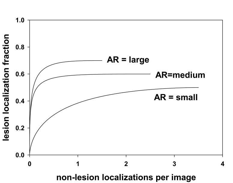
This figure illustrates the effect of choice of acceptance-radius (AR) on scored FROC curves. Shown are three scored FROC curves. The curve labeled “AR = medium” is for a moderate choice of AR. The curve labeled “AR = large” is for a larger choice of AR. It exhibits a higher plateau (more lesion localizations) and a smaller extent along the x-axis (fewer nonlesion localizations). The curve labeled “AR = small” has the opposite characteristics. These curves demonstrate the arbitrary nature of the scored FROC curve, and the consequent arbitrariness of the performance measurement.

To motivate the proposed approach to circumventing the arbitrariness of the choice of the acceptance-radius consider the following question: does a mark scored as a LL actually correspond to the observer seeing the lesion? To address this question we introduce the concepts of perceptual hits and perceptual misses. If the mark resulted from the observer seeing the lesion it is termed a perceptual hit. If the observer did not see the lesion, the mark must have resulted from a non-lesion region that had lesion-like characteristics: this is termed a perceptual miss. It is possible, in fact quite likely, that a perceptual hit will not be at the exact center of the lesion that originated it. If the mark is closer than the acceptance-radius from the lesion center it is scored as a LL and otherwise it is scored as a NL. Conversely a perceptual miss would be scored as a LL if it is inside the acceptance-radius and as a NL otherwise. Therefore, a distinction exists between perceptual events and scored events. If one had a way of estimating the total numbers of perceptual hits and misses, then a perceptual FROC curve could be constructed using these numbers. Unlike a scored FROC curve, such a curve would be independent of acceptance-radius.

Since the truth regarding individual marks, i.e., whether they are perceptual hits or misses is impossible to know, one may question the utility of introducing this distinction. Even if it were practical in observer studies to track the observer's line-of-gaze using eye-tracking apparatus (23), one cannot be 100% certain that a fixation close to a lesion implies that the observer saw the lesion (more on this below). However, the impossibility of knowing the truth does not mean that the concepts of perceptual hits or misses cannot lead to useful results. As an analogy, in ROC methodology one defines a decision variable (24) that is intrinsically unknown (i.e., it is a latent variable) but models employing decision variables have been used with great success to explain observer performance data (14, 25).

The approach taken in this work is to statistically model the spatial distribution of perceptual hits and misses. In other words, if a mark is a perceptual hit, what is the probability that it falls a certain distance from a lesion center? Likewise, what is the probability if a mark is a perceptual miss? The model involves parameters that in principle can be estimated from the observed spatial distribution of the marks. Once the parameters have been determined, one can estimate the most probable total numbers of perceptual hits and misses. Given these numbers one can plot a perceptual FROC operating point. The y-coordinate is the number of perceptual hits normalized by the total number of lesions. The x-coordinate is the number of perceptual misses normalized by the number of images. Since an operating point is determined using the total numbers of perceptual hits and misses, it is not necessary to identify individual marks as perceptual hits or misses. This is fortunate because a statistical method will never be able to identify the truth for individual marks. By varying the criterion used to mark a region (e.g., high confidence, moderate confidence, low confidence) one can plot the perceptual FROC curve. Since the perceptual hits and misses are independent of how one scores the marks, the operating points and the perceptual FROC curve are independent of acceptance-radius.

The methods section amplifies on the concepts of perceptual hits and misses; it describes the rationale for the spatial distribution model; the mathematical details of the model; the estimation procedure and the validation of the model. It shows how one can estimate the most probable number of perceptual hits and misses and generate perceptual FROC operating points and perceptual FROC curves. The rest of the paper describes an application of the method to radiologist generated location data.

2. MATERIALS AND METHODS

Perceptual hits and misses

This section and Fig. 2 are intended to clarify the distinction between a perceptual hit and a perceptual miss. In the present context a mark is defined as a region outlined (or “drawn”) by the observer. When a center is required, it is defined as the centroid of the outlined region. A mark occurs when a region is perceived that is sufficiently suspicious for abnormality to warrant reporting (26, 27). A mark can be either a perceptual hit or a perceptual miss. Simply stated, a perceptual hit occurs when the mark is a result of the observer “seeing” a lesion, and a perceptual miss occurs when the mark is a result of the observer not “seeing” a lesion. In the latter case, since the observer marked the image, a lesion-like non-lesion must have been “seen”. A model of the perceptual process (28-30) suggests that lesions and lesion-like non-lesion regions in the physical image induce disturbances (perturbations) in the observer's internal representation of that image (30). Therefore there are in fact two images, the physical image, labeled “physical” in Fig. 2 and the observer's internal representation of that image, labeled “internal”, which can be regarded as a “virtual” image. The lesion in the physical image is indicated by the shaded area labeled L in Fig. 2. The disturbance in the internal representation is shown by the contour labeled D. The mark in the physical image is the contour labeled M: it is the observer's rendition in the physical image of the disturbance in the internal representation. A perceptual hit occurs when the lesion induces a sufficiently large disturbance in the observer's internal representation as to cause the observer to mark the image. Therefore a perceptual hit can be represented symbolically as L → D → M, as in Fig. 2 (A). Another way of characterizing a perceptual hit is that it was originated or caused by a lesion. A perceptual miss occurs when a non-lesion induces a sufficiently large disturbance in the observer's internal representation as to cause the observer to mark the image. Therefore a perceptual miss can be represented symbolically as N → D → M, as in Fig. 2 (B). A perceptual miss is originated by a non-lesion. A second nonlesion region labeled N2 is also shown in Fig. 2 (B). Note that no corresponding disturbance is shown in the internal representation. This does not mean that the disturbance is zero; rather, the disturbance is not strong enough to have generated a mark. Therefore N2 is not a perceptual miss. Only disturbances strong enough to generate marks are shown if Fig. 2.

Fig. 2.

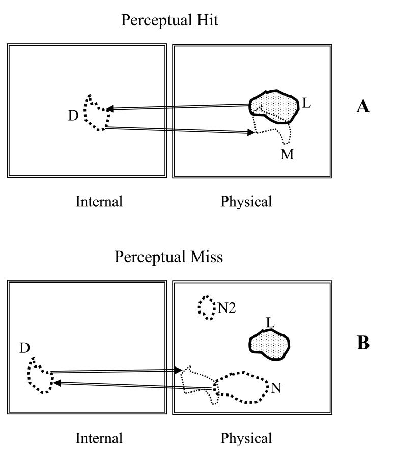
This figure illustrates the distinction between a perceptual hit (upper panel A) and a perceptual miss (lower panel B). Lesions (L) and non-lesions (N) in the physical images (right panels) induce disturbances (D) in the observer's internal representations of the images (left panels). A perceptual hit occurs when the lesion induces a sufficiently large disturbance in the observer's internal representation as to cause the observer to mark the image, schematically L → D → M. A perceptual miss occurs when a non-lesion induces a sufficiently large disturbance in the observer's internal representation as to cause the observer to mark the image, schematically N → D → M. A second non-lesion (N2) shown in B is not a perceptual miss since the disturbance (not shown) is not strong enough to have generated a mark.

The center of a mark is not expected to coincide exactly with the center of the lesion or non-lesion that originated it. If a lesion originated the mark the radiologist traced boundary will not exactly match the true lesion boundary. The radiologist may consider it unnecessary to trace the boundary precisely since the general region may be sufficient to allow another clinician (e.g., the surgeon) to see the same lesion and take appropriate action. Even if the radiologist wishes to mark the region precisely, the boundary in the internal representation may not exactly match the physical boundary. Because of “hand-jitter” the radiologist will not be able to precisely mark the intended region (a CAD system would not have this limitation).

While in Fig. 2 (B) the non-lesion N is shown far from the lesion L, it is possible (but perhaps rare) that it could be very close to it. This would result in a perceptual miss close to the lesion. While it may appear surprising that a lesion and a non-lesion could be close to each other, bear in mind that what constitutes a non-lesion depends on the observer (i.e., the internal representation is observer-dependent). As an example, consider that a resident in training and the supervising mammographer view a mammogram. The resident states that she sees a lesion and points to it and describes its physical characteristics. The mammographer responds “although you are looking in the right place, based on your description you are not seeing the lesion; in fact you are describing a normal anatomic feature that looks to you like a lesion”.

Rationale for the spatial distribution model for the marks

For simplicity assume that each abnormal image has only one lesion. Since regardless of the choice of acceptance-radius a mark on a normal image will always be classified as a NL, it is only necessary to model the spatial distribution of marks relative to lesion centers in abnormal images. The lesion center, defined as the centroid of the lesion boundary, is assumed to be part of the independently determined “truth“ information. For example, the boundary could be the average of several expert radiologist indicated boundaries – the truth panel. Fig. 3 shows a composite stack of images from different patients, each containing a single lesion, where the images have been aligned so that the lesion centers are registered. The common location of the center in Fig. 3 is indicated by the solid dot. The marks in the stacked images are indicated by the “plus” and “minus” symbols. It is assumed that the truth regarding each mark, i.e., whether it was originated by a lesion (perceptual hit) or originated by a non-lesion (perceptual miss), are known. The “plus” symbols represent perceptual hits and the “minus” symbols represent perceptual misses. In the example shown there are 7 perceptual hits and 8 perceptual misses, for a total of 15 marks.

Fig. 3.

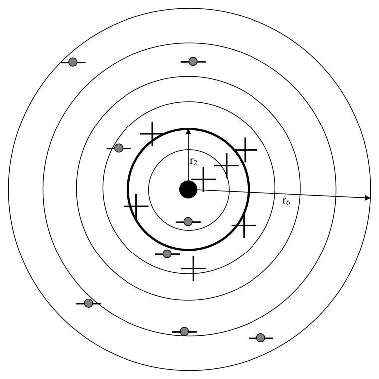
Shown is a “stack” of abnormal images, each with a single lesion, aligned so that the lesion centers, the solid dot, are co-registered. A possible spatial distribution of 15 marks relative to this center is shown. It is assumed that one knows the truth regarding each mark (i.e., whether it is a perceptual hit or a perceptual miss). Shown are 7 perceptual hits (the “plus” symbols) and 8 perceptual misses (the “minus” symbols with the shaded circles). The perceptual hits are shown more tightly clustered around the lesion centers than the perceptual misses. Six (6) radial bins are shown defined by circles with radii r_i, where i = 1, 2, …, 6, two of which are labeled. If the thicker circle with radius r₂ is chosen as the acceptance-radius, then 3 perceptual hits and 1 perceptual miss fall inside this circle and are scored as 4 lesion localizations (LLs). Four (4) perceptual hits and 7 perceptual misses fall outside the acceptance-radius and are scored as 11 non-lesion localizations (NLs). These numbers (4 and 11) determine a scored FROC operating point. The total numbers of perceptual hits and misses (7 and 8, respectively) determine a perceptual operating point. As the acceptance-radius increases the number of LLs increases at the expense of the number of NLs, so the scored point will shift towards the upper-left, but the numbers of perceptual hits and marks remain unaffected, so the perceptual point will not shift.

Two characteristics shown schematically in Fig. 3 are: (a) perceptual hits are clustered around the center, and (b) perceptual misses are more broadly distributed. The first characteristic is expected because each perceptual hit was originated by the lesion in the image. Since the marks are relative to the corresponding lesion center, and if each mark is reasonably close to the lesion center, the stacking operation will result in perceptual hits clustering around the center. The second characteristic, namely the distribution of perceptual misses is relatively broad, may at first sight appear to be unreasonable. Different image regions are not equally susceptible to perceptual misses. For example, in mammography, due to greater anatomic noise, perceptual misses are more likely to occur in the dense glandular regions than in fatty regions. However, while this is true for individual images, the effect of stacking the images, as in Fig. 3, is expected to blur this effect since a glandular region in one image may superpose with a fatty region in another. As more images are included in the stack, the distribution of the marks corresponding to perceptual misses is expected to become broad.

To construct a conventional FROC plot the investigator chooses an acceptance-radius and scores each mark. The mapping from perceptual to scored quantities is determined by the acceptance-radius. The circles in Fig. 3 correspond to concentric radial bins with radii r_i, where i = 1, 2, …, 6. If r₂ is chosen to be the acceptance-radius, then 3 perceptual hits and 1 perceptual miss fall inside this circle. Each of these will be scored as a LL for a total of 4 LLs. The perceptual miss is counted as a LL even though in truth it was originated by a non-lesion. Four (4) perceptual hits and 7 perceptual misses fall outside the acceptance-radius. These will be scored as NLs for a total of 11 NLs. The 4 perceptual hits are counted as NLs even though in truth they were originated by lesions. It is evident that choosing a larger acceptance-radius will increase the number of LLs at the expense of the number of NLs. The mapping from perceptual to scored quantities preserves the total number of perceptual events and marks, i.e., the number of perceptual hits plus the number of perceptual misses equals the number of LLs plus number of NLs (in the example shown in Fig. 3 this number is 15).

If the mark is in fact a perceptual hit and closely matches the physical lesion, the center of the mark is expected to be near the lesion center, an example of which is the “plus” symbol inside the innermost circle in Fig. 3. When there is significant mismatch perceptual hits can occur relatively further from lesion centers, as illustrated by the 4 “plus” symbols in the annulus defined by r₂ and r₃, but on the whole, and as indicated in the figure, perceptual hits are expected to be clustered around the lesion center. One the other hand perceptual misses are expected to be more broadly distributed. Examples of perceptual misses far from the lesion are the 3 “minus” symbols in the outermost annulus in Fig. 3. Occasionally a perceptual miss could occur close to a lesion, an example of which is the “minus” symbol in the innermost circle in Fig. 3.

To summarize, a plausible model for the spatial distribution of the marks has been described. It consists of a narrow distribution centered on the lesion center corresponding to perceptual hits, and a broader distribution corresponding to perceptual misses. The validity of the spatial distribution model can be assessed by statistical methods. One cannot tell for certain from the location of the mark whether it is a perceptual hit or miss. However, statistical methods allow one to determine the most probable numbers of perceptual hits or misses from the observed spatial distribution of the marks. This information allows one to plot a perceptual FROC curve.

Mathematical model for the spatial distribution of the marks

The two dimensional circularly symmetric Gaussian probability density function (pdf) ϕ (r σ) is defined below in Eqn. 1. It has the proper normalization when integrated in two dimensions over all values of r. This function can model a peak with standard deviation σ centered at zero:

$$\begin{array}{cc}\hfill & \varphi (\mathit{r},\sigma )=\frac{1}{2\pi {\sigma }^2}\exp \left(-\frac{r^2}{2{\sigma }^2}\right)\hfill \\ \hfill & {\int }_0^{\infty }2\pi \mathit{r}\varphi (\mathit{r},\sigma )\mathit{dr}=1.\hfill \end{array}$$ Eqn. 1

It is assumed that the spatial distribution of the marks can be modeled by a mixture distribution consisting of two Gaussians of the type described above with standard deviations σ₁ and σ₂ and mixing fraction α. The Gaussians with standard deviations σ₁ and σ₂ correspond to the perceptual hits and misses, respectively, and based on the preceding discussion one expects σ₁ ≪ σ₂, i.e., the spread of the perceptual hits is smaller than that of the perceptual misses. Both Gaussians are centered at the common lesion center in the image stack, the solid dot in Fig. 3, which is defined as the origin of the coordinate system. If the distribution of the perceptual misses is broad, as will be seen to be true for our datasets, it does not matter where it is centered, and for simplicity in modeling we have assumed it is centered at the origin.

The variable α is the probability that a mark is a perceptual hit. The corresponding probability that a mark is a perceptual miss is 1-α. According to the model a perceptual hit could occur at any r, but if σ₁ ≪ 1 it is unlikely to occur far from the center. The integrated probability under the perceptual hit distribution is α, the net probability that a mark is a perceptual hit. Likewise, if σ₂ ≫ 1, a perceptual miss is equally likely to occur anywhere in the image. The integrated probability under the perceptual miss distribution is 1-α, the net probability that a mark is a perceptual miss. It is convenient to bin each mark into one of N_B bins according to its radial distances from the true lesion center (e.g., N_B = 6 in Fig. 3). The distance of a mark from the center of the lesion (in the same image) is r. One defines the binned radius vector $\overrightarrow{\mathit{r}}$

$$\overrightarrow{\mathit{r}}=[{\mathit{r}}_0,{\mathit{r}}_1,\dots ,{\mathit{r}}_{{\mathit{N}}_{\mathit{B}}}],$$ Eqn. 2

where r₀ ≡ 0 and the bin denoted by r₁ is a circle of radius r₁ and the remaining bins are annuli with finite inner radii.

The probabilities f_H (i|α , σ₁) and f_M (i |α , σ₂) of observing perceptual hits or misses in radial bin “i” are given by

$$\begin{array}{cc}\hfill & {\mathit{f}}_{\mathit{H}}(\mathit{i}\mid \alpha ,{\sigma }_1)=\alpha {\int }_{{\mathit{r}}_{\mathit{i}-1}}^{{\mathit{r}}_{\mathit{i}}}2\pi \mathit{r}\varphi (\mathit{r},{\sigma }_1)\mathit{dr}\hfill \\ \hfill & {\mathit{f}}_{\mathit{M}}(\mathit{i}\mid \alpha ,{\sigma }_2)=(1-\alpha ){\int }_{{\mathit{r}}_{\mathit{i}-1}}^{{\mathit{r}}_{\mathit{i}}}2\pi \mathit{r}\varphi (\mathit{r},{\sigma }_2)\mathit{dr},\hfill \end{array}$$ Eqn. 3

where i = 1, 2, …, N_B. It is assumed that ${\mathbf{r}}_{N_B}\gg {\sigma }_2>{\sigma }_1$ so as that all of the integrated areas under the pdfs are included, i.e.,

$$\begin{array}{cc}\hfill & \alpha {\int }_{{\mathit{r}}_0}^{{\mathit{r}}_{{\mathit{N}}_{\mathit{B}}}}2\pi \mathit{r}\varphi (\mathit{r},{\sigma }_1)\mathit{dr}=\alpha \hfill \\ \hfill & (1-\alpha ){\int }_{{\mathit{r}}_0}^{{\mathit{r}}_{{\mathit{N}}_{\mathit{B}}}}2\pi \mathit{r}\varphi (\mathit{r},{\sigma }_2)\mathit{dr}=1-\alpha .\hfill \end{array}$$ Eqn. 4

Determination of the parameters

The observed vector $\overrightarrow{\mathit{N}}$ of marks is defined by

$$\overrightarrow{\mathit{N}}=[{\mathit{N}}_1,{\mathit{N}}_2,\dots ,{\mathit{N}}_{{\mathit{N}}_{\mathit{B}}}],$$ Eqn. 5

where N_i is the number of marks in bin i (e.g., in Fig. 3, N₃ = 6 ). Assuming independence, the probability of observing a mark in bin “i”, regardless of whether it is a hit or a miss, is given by

$$\mathit{P}(\mathit{i}\mid \alpha ,{\sigma }_1,{\sigma }_2)={\mathit{f}}_{\mathit{H}}(\mathit{i}\mid \alpha ,{\sigma }_1)+{\mathit{f}}_{\mathit{M}}(\mathit{i}\mid \alpha ,{\sigma }_2).$$ Eqn. 6

Assume that the numbers of marks N_i in the different bins are independent. The probability of observing the data vector $\overrightarrow{\mathit{N}}$ is given by (ignoring factors that are independent of the parameters σ₁, σ₂ and α)

$$\mathit{P}(\overrightarrow{\mathit{N}}\mid \alpha ,{\sigma }_1,{\sigma }_2)=\prod _{\mathit{i}=1}^{{\mathit{N}}_{\mathit{B}}}{\left[\mathit{P}(\mathit{i}\mid \alpha ,{\sigma }_1,{\sigma }_2)\right]}^{{\mathit{N}}_{\mathit{i}}}.$$ Eqn. 7

The total number of marks in the data set is N, where

$$\mathit{N}=\sum _{i=1}^{{\mathit{N}}_{\mathit{B}}}{\mathit{N}}_{\mathit{i}}.$$ Eqn. 8

The log-likelihood function is given by

$$\mathit{LL}\equiv \mathit{LL}(\overrightarrow{\mathit{N}}\mid \alpha ,{\sigma }_1,{\sigma }_2)=\sum _{i=1}^{{\mathit{N}}_{\mathit{B}}}{\mathit{N}}_{\mathit{i}}\log \left(\mathit{P}(\mathit{i}\mid \alpha ,{\sigma }_1,{\sigma }_2)\right).$$ Eqn. 9

.

The parameters of this model, σ₁, σ₂ and α, can be determined by maximizing the log-likelihood function with respect to these parameters. In this work we used the method of simulated annealing as implemented in the GNU library (31) to minimize the negative of log-likelihood (−LL). The starting parameter values were σ₁ = 0.05, σ₂ = 2.0 and α = 0.8. The final estimates were insensitive to different choices of starting values suggesting that the algorithm was not finding local minima. The covariance matrix is the inverse of the expectation value of the matrix of second partial derivatives of −LL with respect to the parameters, evaluated at the final parameter values (32). The diagonal elements of the covariance matrix are the variances of the parameter estimates.

Determination of the most probable values of perceptual hits and misses

The total number of marks N_i in the i^th bin is the sum of two terms, ${\mathit{N}}_{\mathit{i}}^{\mathit{H}}$ and ${\mathit{N}}_{\mathit{i}}^{\mathit{M}}$, corresponding to the perceptual hits and misses, respectively:

$${\mathit{N}}_{\mathit{i}}={\mathit{N}}_{\mathit{i}}^{\mathit{H}}+{\mathit{N}}_{\mathit{i}}^{\mathit{M}}$$ Eqn. 10

Due to the stochastic nature of the problem it is not possible to determine if any individual mark is a perceptual hit or a miss. The most probable number (an integer) of perceptual hits ${\mathit{N}}_{\max ,\mathit{i}}^{\mathit{H}}$ in the i^th bin can be determined as follows. The probability of observing ${\mathit{N}}_{\mathit{i}}^{\mathit{H}}$ perceptual hits in the i^th bin is given by

$$\mathit{P}({\mathit{N}}_{\mathit{i}}^{\mathit{H}}\mid {\mathit{N}}_{\mathit{i}},\alpha ,{\sigma }_1,{\sigma }_2)=\frac{{\mathit{N}}_{\mathit{i}}!}{{\mathit{N}}_{\mathit{i}}^{\mathit{H}}!({\mathit{N}}_{\mathit{i}}-{\mathit{N}}_{\mathit{i}}^{\mathit{H}})!}{\left[{\mathit{f}}_{\mathit{H}}(\mathit{i}\mid \alpha ,{\sigma }_1)\right]}^{{\mathit{N}}_{\mathit{i}}^{\mathit{H}}}{\left[{\mathit{f}}_{\mathit{M}}(\mathit{i}\mid \alpha ,{\sigma }_2)\right]}^{{\mathit{N}}_{\mathit{i}}-{\mathit{N}}_{\mathit{i}}^{\mathit{H}}}.$$ Eqn. 11

This leads to the following expression for the log-likelihood function $\mathit{LL}\left({\mathit{N}}_{\mathit{i}}^{\mathit{H}}\mid {\mathit{N}}_{\mathit{i}},\alpha ,{\sigma }_1,{\sigma }_2\right)$

$$\begin{array}{cc}\hfill & \mathit{LL}\left({\mathit{N}}_{\mathit{i}}^{\mathit{H}}\mid {\mathit{N}}_{\mathit{i}},\alpha ,{\sigma }_1,{\sigma }_2\right)=-\log \left[{\mathit{N}}_{\mathit{i}}^{\mathit{H}}!\right]-\log \left[\left({\mathit{N}}_{\mathit{i}}-{\mathit{N}}_{\mathit{i}}^{\mathit{H}}\right)!\right]+{\mathit{N}}_{\mathit{i}}^{\mathit{H}}\log \left[{\mathit{f}}_{\mathit{H}}(\mathit{i}\mid \alpha ,{\sigma }_1)\right]\hfill \\ \hfill & +\left({\mathit{N}}_{\mathit{i}}-{\mathit{N}}_{\mathit{i}}^{\mathit{H}}\right)\log \left[{\mathit{f}}_{\mathit{M}}(\mathit{i}\mid \alpha ,{\sigma }_2)\right],\hfill \end{array}$$ Eqn. 12

where only terms involving ${\mathit{N}}_{\mathit{i}}^{\mathit{H}}$, the quantity to be estimated, have been retained. The most probable value of ${\mathit{N}}_{\mathit{i}}^{\mathit{H}}$ can be found by determining the integer value of ${\mathit{N}}_{\mathit{i}}^{\mathit{H}}$ that yields the largest value of $\mathit{LL}\left({\mathit{N}}_{\mathit{i}}^{\mathit{H}}\mid {\mathit{N}}_{\mathit{i}},\alpha ,{\sigma }_1,{\sigma }_2\right)$, i.e.,

$${\mathit{N}}_{\max ,\mathit{i}}^{\mathit{H}}=\begin{array}{c}\hfill \arg \max \hfill \\ \hfill {\mathit{N}}_{\mathit{i}}^{\mathit{H}}\hfill \end{array}\left(\mathit{LL}\left({\mathit{N}}_{\mathit{i}}^{\mathit{H}}\mid {\mathit{N}}_{\mathit{i}},\alpha ,{\sigma }_1,{\sigma }_2\right)\right).$$ Eqn. 13

Note that this maximization is performed using the values for σ₁, σ₂ and α determined above. The corresponding value of ${\mathit{N}}_{\max ,\mathit{i}}^{\mathit{M}}$ is ${\mathit{N}}_{\mathit{i}}-{\mathit{N}}_{\max ,\mathit{i}}^{\mathit{H}}$. The expected values of ${\mathit{N}}_{\mathit{i}}^{\mathit{H}}$ and ${\mathit{N}}_{\mathit{i}}^{\mathit{M}}$ are given by

$$\langle {\mathbf{N}}_{\mathbf{i}}^{\mathbf{H}}\rangle =\mathbf{N}•{\mathbf{f}}_{\mathbf{H}}(\mathbf{i}\mid \alpha ,{\sigma }_1),$$ Eqn. 14

and

$$\langle {\mathbf{N}}_{\mathbf{i}}^{\mathbf{M}}\rangle =\mathbf{N}•{\mathbf{f}}_{\mathbf{M}}(\mathbf{i}\mid \alpha ,{\sigma }_2).$$ Eqn. 15

These values will in general be non-integers and will satisfy

$$\sum _{\mathbf{i}=1}^{N_B}\left(\langle {\mathbf{N}}_{\mathbf{i}}^{\mathbf{H}}\rangle +\langle {\mathbf{N}}_{\mathbf{i}}^{\mathbf{M}}\rangle \right)<\mathbf{N}.$$ Eqn. 16

This is because not all of the integral under the Gaussian distributions will be accounted for with a finite number of bins.

Validity of the model

The statistical validity of the model was assessed by computing the Pearson goodness of fit statistic χ² (33):

$${\chi }^2=\sum _{\mathbf{i}=1}^{\mathbf{i}=N_B}\left[\frac{{\left({\mathbf{N}}_{\mathbf{i}}-\langle {\mathbf{N}}_{\mathbf{i}}\rangle \right)}^2}{\langle {\mathbf{N}}_{\mathbf{i}}\rangle }\right]$$ Eqn. 17

The expected value of N_i is given by

$$\langle {\mathbf{N}}_{\mathbf{i}}\rangle =\mathbf{N}•\mathbf{P}(\mathbf{i}\mid \alpha ,{\sigma }_1,{\sigma }_2)=\mathbf{N}•\left({\mathbf{f}}_{\mathbf{H}}\left(\mathbf{i}\mid \alpha ,{\sigma }_1\right)+{\mathbf{f}}_{\mathbf{M}}\left(\mathbf{i}\mid \alpha ,{\sigma }_2\right)\right).$$ Eqn. 18

The number of degrees of freedom df associated with χ² is df = N_B - 1 - 3 , i.e., df = N_B - 4. The χ² statistic is valid if the expected number of marks in each bin is at least five (33) and when this is not true one needs to cumulate bins (this will decrease N_B). Define ${\chi }_{\mathit{df}}^2$ as the chi-square distribution pdf for df degrees of freedom (33). Then, at the α level of significance, the null hypothesis that the estimated parameter values are identical to the true values is rejected in favor of the hypothesis that at least one of them is different if χ² >χ² _1–α,df, where χ²_1–α,df is the critical value such that the integral of ${\chi }_{\mathit{df}}^2$ from 0 to χ² _1–α,df equals 1-α. The observed value of χ² can be converted to a significance value (p-value) from χ² = χ² _1–α,df. At the 5% significance level, if p < 0.05, then one rejects the null hypothesis, i.e., the fit is not good. In practice one often accepts p-values as small as 0.001 as evidence of a reasonable fit (34, 35).

Constructing perceptual FROC curves

A multi-rating free-response study corresponds to multiple cutoffs ζ_j where j = 1, 2, .., R and R is the number of ratings bins. The procedure for constructing a perceptual FROC curve from a multi-rating study is as follows. For each j one determines the total number of marks in ratings bins j and above. This suffices to determine the parameters ${\sigma }_1^j$, ${\sigma }_2^j$ and α^j of the spatial localization model (all parameters of the model are potentially rating dependent). These parameters yield the most probable numbers of perceptual hits and misses, Eqn. 13. The y-coordinate of the perceptual FROC operating point is given by

$${\mathit{y}}_{\mathit{p}}\left({\zeta }_{\mathit{j}}\right)==\frac{{\displaystyle \sum _{\mathit{i}=1}^{{\mathit{N}}_{\mathit{B}}}}{\mathit{N}}_{\max ,\mathit{i}}^{\mathit{H},\mathit{j}}}{{\mathit{N}}_{\mathit{L}}},$$ Eqn. 19

where ${\mathit{N}}_{\max ,\mathit{i}}^{\mathit{H},\mathit{j}}$ is the most probable number of cumulated (i.e., rating j and above) perceptual hits in radial bin i, and N_L is the total number of lesions. The x-coordinate of the perceptual FROC operating point is given by

$${\mathit{x}}_{\mathit{p}}\left({\zeta }_{\mathit{j}}\right)=\frac{{\displaystyle \sum _{\mathit{i}=1}^{{\mathit{N}}_{\mathit{B}}}}{\mathit{N}}_{\max ,\mathit{i}}^{\mathit{M},\mathit{j}}}{{\mathit{N}}_{\mathit{I}}},$$ Eqn. 20

where ${\mathit{N}}_{\max ,\mathit{i}}^{\mathit{M},\mathit{j}}$ is the most probable number of cumulated (i.e., rating j and above) perceptual misses in radial bin i, and N_I is the total number of images. The subscript p denotes that these are perceptual values, not acceptance-radius-dependent scored values. The superscript j denotes that the values pertain to rating j and above. The procedure is repeated for all cutoffs adopted by the observer to yield R perceptual operating points. If the cutoffs are closely spaced and one has many images, one can in principle generate a perceptual FROC curve. Alternatively, if one has a method of fitting the data points to a theoretical model (6, 9-11), one can generate a theoretical perceptual FROC curve using fewer images and a finite number of ratings bins.

Observer Study

Nine (9) observers participated in the observer study, which was part of a larger study involving eye-position recordings (36). Three were experienced dedicated mammographers with at least 3 years experience reading mammograms, from the Department of Radiology, University of Pennsylvania, and six were radiology residents undergoing mammography rotation. The resident's experience reading mammograms ranged from 302 to 976 cases, whereas the mammographers typically read between 3,000 and 5,000 mammograms per year. For the purpose of analysis the radiology residents were subdivided into 2 groups: three residents were in their second mammography rotation and were considered ‘more experienced’, and three residents were in their first mammography rotation and were considered ‘less experienced’. The groups are referred to as A, B and C, where A represents the mammographers, B the more experienced residents and C the less experienced residents.

The observers viewed 19 two-view (craniocaudal, CC, and mediolateral-oblique, MLO) breast images. Each breast contained a single malignant lesion that was visible in both views to an experienced mammographer. There were 12 cases with masses and 6 cases with calcification clusters and one case had an architectural distortion. The average mass size was 0.37° (range 0.21° – 0.73°) and the average size of the remaining lesions was 0.33° (range 0.16° to 0.7°). All lesion dimensions in this paper are in degrees of visual angle subtended at the retina at an average viewing distance of 38 cm (e.g., a 1 cm mass subtends 1.5° of visual angle at the retina). The observers were not constrained to exactly this viewing distance; for comfort they were allowed small head movements.

The images were digitized using a Lumisys Model 100 digitizer (Lumisys Inc, Sunnyvale, CA), with a pixel size of 50μm × 50μm and a gray level resolution of 12 bits. The two-view mammogram cases were displayed on a 21-inch landscape-mode monitor with 2560 × 2048 pixels (Model DS5000L, Clinton Electronics, Rockford, IL). Regardless of whether the image displayed was of the left or the right breast, the CC view always appeared in the left half and the MLO view always appeared in the right half of the display. The observers were instructed to mark regions that were suspicious for malignancies, and to mark them on both views, even if they thought they belonged to the same lesion. They were not asked to rated the suspicious regions. Each observer indicated, using the cursor and in both views, all suspicious regions that in their opinion were clinically reportable. They were instructed to click at the center of each suspicious region. An experienced mammographer, using pathology reports and additional films, marked the coordinates of all malignancies in the cases in both views. This was done two years prior to the observer study. This mammographer was asked to place the marks as close as possible to the ‘centers’ of the lesions. This mammographer also participated in the observer study, but memory effects were expected to be minimal due to the large amount of time that elapsed between marking the ‘truth’ and reading the images.

The distance between any mark made by the observer and the lesion center was binned into one of 40 bins (i.e., N_B =40). Each bin corresponded to 0.25° of visual angle. Thus, if the observer's mark fell between 0° and 0.25° from the lesion center the bin-count in the first bin was incremented by unity, and so on. The choice of 0.25° for the bin-size was a compromise between too few marks in individual bins (excessively small bin-size) and loss of spatial localization resolution (excessively large bin-size). The value N_B = 40 ensured that the largest breast in the cases was encompassed by r₄₀. By pooling data from different observers the data vectors $\overrightarrow{\mathit{N}}$ for each observer group (A, B, and C) were generated. The analysis then proceeded along the lines described above.

RESULTS

Fig. 4 shows the histogram of the numbers of marks in the radial bins for observer group A, the three experienced mammographers. Each bin has a width of 0.25° and the total number of marks for this group was 113, see Table 1. The dotted line is the theoretical fit to the histogram, i.e., Eqn. 18. This group generated more marks than the other groups. Fig. 5 shows corresponding plots for group B, the three more experienced residents. The total number of marks for this group was 104. Fig. 6 applies to group C, the three least experienced residents. The total number of marks for this group was 73. This group generated the least number of marks. The overall shapes of the theoretical fits for all three groups were similar. Each shows an initial sharp decrease leading to a minimum near the origin, a subsequent increase and a broad peak at approximately bin number 15 to 20, and this shape will be explained below.

Fig. 4.

This figure shows the histogram of the observed number of marks in the radial bins for group A, the three experienced mammographers. Each bin has a width of 0.25° and the total number of marks for this group was 113. The dotted line is the theoretical fit to the histogram, i.e., Eqn. 18. The parameters of the fit are α = 0.53, σ₁ = 0.14 and σ₂ = 3.2, and the goodness of fit statistics are χ² = 15, df = 6 and p-value = 0.02, indicative of a good fit, as is also evident from the visual impression of this figure. The shape of the theoretical fit, namely the sharp minimum at bin ∼ 3, the subsequent rise and the broad peak at bin ∼15, is explained in the text.

Table 1.

Total number of marks in the different bins (column 3), the most probable number of perceptual hits and misses (columns 4 and 5), and the expected numbers of perceptual hits and misses (columns 6 and 7), for the three observer groups. Group A represents the mammographers, group B the more experienced residents, and group C the less experienced residents. The sum of the perceptual hits and misses over all bins determines the perceptual operating points shown in Fig. 7. If the 4^th bin is chosen as the acceptance criterion, the sum of the observed number of marks (column 3) for the first 4 bins determines the ordinate of the scored operating point, and the corresponding sum over the remaining bins determines the abscissa, see Fig. 7.

Observer Group	Bin index, i	Observed number of marks	Most probable		Expected
			Perceptual hits,${\mathit{N}}_{\max ,\mathit{i}}^{\mathit{H}}$	Perceptual misses,${\mathit{N}}_{\max ,\mathit{i}}^{\mathit{M}}$	Perceptual hits,$\langle {\mathit{N}}_{\mathbf{i}}^{\mathbf{H}}\rangle$	Perceptual misses,$\langle {\mathit{N}}_{\mathbf{i}}^{\mathit{M}}\rangle$
A	1	50	50	0	48.3	0.163
	2	10	10	0	11.8	0.487
	3	7	0	7	0.090	0.802
	4	4	0	4	0	1.102
	5-40	42	0	42	0	49.9
B	1	36	36	0	35.4	0.146
	2	6	6	0	6.26	0.437
	3	7	0	7	0.0215	0.721
	4	3	0	3	0	0.996
	5-50	52	0	52	0	58.6
C	1	22	22	0	16.4	0.0964
	2	6	6	0	13.7	0.288
	3	5	4	1	1.69	0.475
	4	3	0	3	0	0.828
	5-40	37	0	37	0	37.8

Fig. 5.

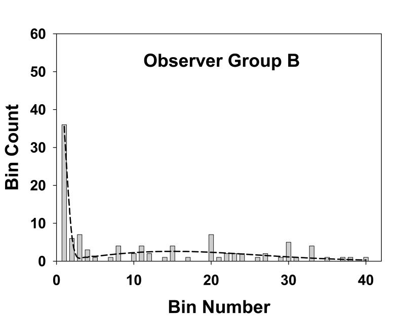
This figure is similar to Fig. 4, except that it applies to group B, the three more experienced residents. The total number of marks for this group was 104. The parameters of the fit are α = 0.40, σ₁ = 0.13 and σ₂ = 3.7, and the goodness of fit statistics are χ² = 15, df = 8 and p-value = 0.06, also indicative of a good fit.

Fig. 6.

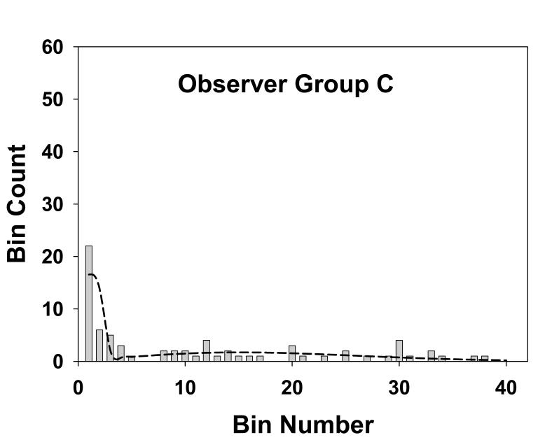
This figure is similar to Fig. 4, except that it applies to group C, the three least experienced residents. The total number of marks for this group was 73. The parameters of the fit are α = 0.44, σ₁ = 0.21 and σ₂ = 3.7, and the goodness of fit statistics are χ² = 20, df = 5 and p-value = 0.001, indicative of a poor fit, although the visual impression is that the fit is not unreasonable.

The observed numbers of marks is also shown in the third column of Table 1 where, for convenience in displaying the data bins 5-40 are treated as a single bin, somewhat obscuring the fact that some of the original bins had no marks, as evident from Figs. 4, 5 and 6. Columns 4 and 5 in Table 1 list the most probable numbers (Eqn. 13) of perceptual hits and misses, respectively, in the different bins. Columns 6 and 7 list the corresponding expected numbers (Eqn. 14 and 15). The total expected number of marks for groups A, B and C were 112.6, 102.6 and 71.3, respectively. These values are slightly smaller than the corresponding observed numbers (113, 104 and 73) which is due to the perceptual misses distribution having a small tail beyond the 40^th bin, see Eqn. 16.

Table 2 summarizes the estimated parameter values (i.e., σ₁, σ₂ and α) and corresponding 95% confidence intervals (in parentheses) for mammographers (group A), residents with more experience (group B) and residents with less experience (group C). The σ₁ and σ₂ values, representing the spread of marks representing perceptual hits and misses, were similar for all groups. The marginally higher value of σ₁ for group C is within the range of uncertainty. The α values, the probability that a mark is a perceptual hit, were also similar for all groups (group A is marginally higher). The model fits are reasonable for groups A and B (p-values of 0.02 and 0.06, respectively) and poor for group C (p-value = 0.001). Visual inspection of Figs. 4, 5 and 6 indicate that in all cases the fits are reasonably consistent with the data. For the purpose of calculating χ² adjacent bins were combined to yield a minimum of 5 expected marks. This procedure yielded varying numbers of combined bins for the different groups. This is evident from the varying degrees of freedom (df) values listed in Table 2. For example, for group A (df = 6) the total number of bins was N_B = 6 + 4 = 10. The 10 combined bins were as follows: bin 1, bins 2 through 5, bins 6 through 8, bins 9 through 11, bins 12 through 13, bins 14 through 16, bins 17 through 19, bins 20 through 22, bins 23 through 27 and bins 28 through 40. The specific bins that were combined were different for the three groups.

Table 2.

Estimated parameter values, 95% confidence intervals (in parentheses) and goodness of fit statistics (last column) for the 3 groups of observers. The fits are good for groups A and B and marginal for group C, as also seen visually in Figs. 4, 5 and 6. The σ₂ values (spread of the perceptual misses) are similar for all groups, group C had a marginally larger σ₁ value (spread of the perceptual misses) and group A had a marginally higher α value (probability that a mark is a perceptual hit). None of the differences were significant.

Observer group	number of marks N	Model parameters			goodness of fit χ2/ df / p-value
		σ1	σ2	α
A	113	0.14 (0.022)	3.2 (0.46)	0.53 (0.096)	15.0 / 6 / 0.02
B	104	0.13 (0.026)	3.7 (0.51)	0.40 (0.098)	15.0 / 8 / 0.06
C	73	0.21 (0.046)	3.7 (0.63)	0.44 (0.12)	19.8 / 5 / 0.001

Fig. 7 shows operating points labeled A, B and C (the large open circles) for the three groups of observers. Since in this study no rating was provided (this is equivalent to a single rating free-response study) one cannot plot perceptual FROC curves. The curves shown in Fig. 7 are theoretical FROC curves according to a search-model (26, 27). The parameters of the search model were adjusted to yield the two curves shown. The first curve had the property that it passed through point A. The second curve passed through points B and C. These curves are for illustrative purposes only as many choices of search-model parameters yielding curves with the stated properties were possible, especially for point A. To emphasize an essential difference (i.e., the perceptual quantities do not involve scoring) the axes of the perceptual FROC curve are labeled perceptual misses per image and perceptual hit fraction in Fig. 7, whereas the axes of a scored FROC curve, which is acceptance-radius-dependent, are labeled non-lesion localizationsper image and lesion localization fraction in Fig. 1. The smaller filled circles in this plot, labeled a′, b′ and c′, are scored operating points that result if one chooses 4 bins (i.e., 1°) as the acceptance-radius (this is explained below).

Fig. 7.

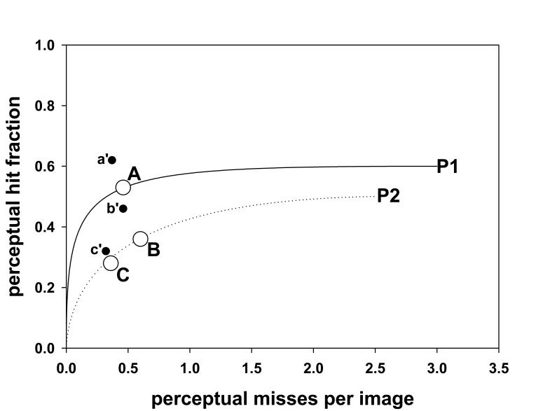
Shown are two perceptual FROC curves, labeled P1 and P2. The axes of a perceptual FROC plot are x: perceptual hit fraction and y: perceptual misses per images. The circles A, B and C are perceptual FROC operating points corresponding to the three groups. The curves P1 and P2 are hypothetical perceptual FROC curves. These curves suggest that groups B and C are performing equivalently and that group A has superior performance. Note the difference in labeling of the axes in this figure as compared to Fig. 1. The filled circles in this plot, labeled a′, b′ and c′, are scored operating points, corresponding to the observer groups A, B and C, respectively, that result if one chooses 4 bins (i.e., 1°) as the acceptance angle. Note the shift towards (0, 1) of each scored point relative to the corresponding perceptual point (compare to Fig. 1 “medium” →“large”), suggesting that this choice of acceptance angle will overestimate true performance.

Regarding the effect of bin-size, as long as the bins are not too large, one expects the integral under the perceptual hits distribution, and consequently α, to be unaffected. With small bin-size there is a point of diminishing returns, as this would result in more bins with no marks, and these bins do not contribute to the log-likelihood function, see Eqn. 9. Similarly, since the parameters σ₁ and σ₂ in Table 2 are in degrees of visual angle, they too should be unaffected. As a test the data for group C was analyzed with bin-size = 0.5° corresponding to N_B = 20 bins. The results for the parameters α, σ₁ and σ₂ (and the 95% confidence intervals) were 0.48 (0.12), 0.28 (0.06) and 3.8 (0.68), respectively. The values are identical, to within the stated precision, to the group C values listed in Table 2.

DISCUSSION

This work describes a method for modeling the spatial distribution of marks in a free-response study. Two concepts are introduced – that of perceptual hits and perceptual misses. A perceptual hit is a mark made as a result of the observer seeing a lesion. A perceptual miss is a mark made as a result of the observer seeing a non-lesion. The modeling is indifferent to how the observer saw the lesion or non-lesion, i.e., whether it was seen using foveal or peripheral vision. It should be emphasized that the present approach is not about finding an optimal acceptance-radius – rather it is about an analysis scheme that does not even use the concept of an acceptance-radius. It is also worth noting that non-lesion regions that are evaluated but not marked, often termed true-negatives, are not part of the free-response dataset and consequently are not the subject of the analysis described in this work.

The model consists of a mixture of two Gaussians characterized by three parameters σ₁, σ₂ and α. The parameter α is the probability that a mark made by an observer is a perceptual hit (1-α is the probability of a perceptual miss). The σ₁ parameter describes the spread of the perceptual hits. The σ₂ parameter describes the spread of the perceptual misses. A procedure is described for estimating the model parameters from free-response data. The perceptual hits distribution is expected to be narrower than that for perceptual misses, i.e., σ₁ ≪ σ₂. This is evident in Figs. 4, 5 and 6 and Table 2. Specifically, Table 2 shows that for experienced mammographers σ₁ = 0.14 and σ₂ = 3.2, i.e., the perceptual misses distribution is more than 20 times wider than the perceptual hits distribution. The σ₂ values for the different groups were similar, i.e., when the observers did not see the lesion, the spread of the marks was independent of expertise – a perhaps not unexpected finding (expertise-dependent correlations between marks and lesion centers are expected to average out in the stacking). Another finding evident from Table 2 is that σ₁ for experienced mammographers (group A) and experienced residents (group B) are similar and marginally smaller than σ₁ for first year residents (group C). This is consistent with the notion that with experience the radiologist is able to better see the lesion, and therefore more accurately mark it, whereas the first year residents are relatively poorer at this task. The α parameter shows an increasing trend with experience, particularly for the experienced mammographers. The number of marks showed an increasing trend with experience (N = 73, 104 and 113 for groups C, B and A, respectively). Together with the observed trends in the model parameters, this resulted in greater numbers of marks that were closer to the lesion centers as experience increased (see Figs. 4, 5 and 6).

In connection with Figs. 4, 5 and 6 it was noted above that in each case the fitted curve shows an initial sharp decrease leading to a minimum near the origin, a subsequent increase and a broad peak at approximately bin number 15 to 20. According to Table 2, 1° visual angle (bin 4) corresponds to between 5 to 7 times σ₁. Therefore the probability of a perceptual hit outside bin 4 is practically zero. Therefore the initial sharp decrease corresponds to the perceptual hits and the remainder of the curve corresponds to perceptual misses. The explanation for the subsequent increase and the broad peak for the perceptual misses is due to the competition between the r term in the integrand of Eqn. 4, which increases with bin number, and the Gaussian term, which decreases with bin number and eventually wins. Based on this logic a second peak at small radius (≪1°) is also expected for the perceptual hits, but due to the finite size of the first bin (0.25°) the expected downturn as r approaches zero is smeared out.

For group A the total of the most probable numbers of perceptual hits summed over all bins is 60, see Table 1. Since this group made 113 marks the probability of a perceptual hit is 60 / 113 = 0.53, which is identical to the estimated value α = 0.53 for this group listed in Table 2. Similar agreements were observed for groups B and C. These agreements are not fortuitous and simply reflect internal consistency of the modeling. Group C illustrates an interesting point: bin 3 for this group has 4 perceptual hits and one perceptual miss. One does not know which of the 5 marks in this bin is a perceptual hit and which is a miss. One only knows the most probable numbers, 4 and 1 in this case.

The estimated most probable number of marks (columns 4 and 5 in Table 1) can be used to infer perceptual FROC operating points (x_p, y_p). In the present case the number of lesions N_L = 2 × 19 × 3 = 114 (i.e., 1 lesion per view, two views per breast, 19 breasts, 3 radiologists per group). Therefore, using Eqn. 19, for group A one has y_p = 60 / 114 = 0.53 perceptual hits per lesion (since 113 ∼114 this value is coincidentally close to α). Since 53 perceptual misses (see Table 1 column 5) occurred in a total of 114 images (in this study the number of images equaled the number of lesions), the x-coordinate is x_p = 53 / 114 = 0.46 perceptual misses per image (Eqn. 20). The corresponding (x_p, y_p) values for groups B and C are (0.60, 0.36) and (0.36, 0.28), respectively. The curves shown in Fig. 7 are theoretical FROC curves according to a search-model (26, 27). The fact that the operating points labeled B and C lie on a single FROC curve suggests that performances of the two groups of residents are similar. The only difference between them is in the operating point: the more experienced residents were more aggressive in reporting lesions. The mammographers, on the other hand, showed superior performance compared to the other groups. This finding is not unexpected given the huge difference in numbers of cases read by this group (between 9,000 and 25,000) as compared to the residents (between 302 and 976).

By adopting a scoring criterion, one can also obtain conventional FROC data points. Inspection of Fig. 4, 5 and 6 suggests that 4 bins (i.e., 1°) is a reasonable acceptance-radius. The corresponding number of LLs for an observer is obtained by summing the values in the first 4 bins in column 3 of Table 1 for this observer. The number of NLs is the sum of the remaining bins. Therefore the scored operating points (x_s, y_s) for groups A, B and C are (0.37, 0.62), (0.46, 0.46) and (0.32, 0.32), respectively. The subscript s denotes that these are scored quantities. As noted above, the corresponding perceptual operating points (x_p, y_p) are (0.46, 0.53), (0.60, 0.36) and (0.36, 0.28). In each case the scored y-coordinate (lesion localization fraction) is greater than the corresponding perceptual y-coordinate (perceptual hit fraction) and the scored x-coordinate (non-lesion localizations per image) is smaller than the corresponding perceptual x-coordinate (perceptual misses per image). In other words the scored point is shifted towards (0, 1) relative to the corresponding perceptual point. This suggests that an acceptance angle of 1° will overestimate performance, see curve labeled “AR = large” in Fig. 1. Adoption of a smaller acceptance criterion, e.g., 1 bin, would have led to the opposite effect, see curve labeled “AR = small” in Fig. 1, suggesting that an acceptance angle of 0.25° will underestimate performance. These results suggest that one cannot estimate true performance using scored FROC curves and one cannot compare scored FROC curves from different studies using different scoring criteria. However, comparisons of different readers and modalities using the same set of cases and the same acceptance-radius criterion are probably valid. The result that a 1° acceptance angle appears to be too large in our case may surprise researchers engaged in eye-movement studies, where a criterion of 2.5° of visual angle is commonly used. This could be because the lesions used in this work are smaller than is typical.

In our opinion, the significance of this study is showing that it is possible to infer perceptual quantities, namely the most probable numbers of perceptual hits and misses, from physically observed location data. These numbers allow one to plot a perceptual FROC operating point that is independent of the choice of acceptance-radius. In a multi-rating FROC study the most probable numbers of perceptual hits and misses for each cutoff could be analyzed by several methods (6, 9-11) to yield fitted FROC curves and estimates of observer performance. For multiple-reader multiple-case (MRMC) free-response studies the data could be analyzed along the lines of the Dorfman, Berbaum and Metz (DBM) method (37) to perform significance testing of the differences in performance between modalities. The fitted curves, the performance estimates and the significance testing would all be independent of acceptance-radius. Applications of the methodology need not be limited to free-response data. For example, in eye-movement studies (23) it is common to assign an acceptance “angle” criterion, and regard a fixation closer than, for example, 2.5° of visual angle from a lesion center as evidence that the observer “found” the lesion (38). This work could be used to perform a statistical classification of fixations without having to adopt an arbitrary acceptance angle criterion. The method does not allow the investigator to identify individual fixations as perceptual hits or misses. In our opinion no method can tell with 100% certainty whether an individual fixation is a perceptual hit or miss.

Among study limitations, this study is based on a limited number of cases, only 19. The independence assumptions of the underlying model are probably violated: the marks are not independent since three observers in each group interpreted a common set of images, and each image (view) was shown simultaneously with the other view. Given the small number of images we had no choice but to pool the numbers. The lesion centers were indicated by only one mammographer: ideally a truth panel consensus is desirable. The spatial distribution model is currently limited to images with one lesion. However, multiple marks in the same vicinity, even overlapping outlined regions, are accommodated by the modeling. We did not correct for lesions located near the boundary of the breast region. These are expected to violate the circular symmetry assumption inherent in the model (the 2π factor in some of the equations). Only abnormal images were used in this analysis. Information from normal images, if successfully incorporated in the model, are expected to yield more reliable results, particularly regarding the magnitude of σ₂. Since resident training methods vary between institutions, the conclusions relating to the effect of experience may be specific to the institution at which the observer data was collected. In certain free-response studies one does not collect the data in the form of individual marks. Rather, the radiologist is asked to localize suspicious regions, if found, to one of a finite number of investigator specified areas. These areas are often chosen based on clinical criteria and the knowledge that precise localization is unnecessary for certain clinical interventions. Finally, since we did not collect rating data, it was not possible to plot more than one FROC operating point per observer group; therefore we could not show fitted FROC curves.

REFERENCES

- 1.Egan JP, Greenburg GZ, Schulman AI. Operating characteristics, signal detectability and the method of free response. J Acoust Soc. Am. 1961;33:993–1007. [Google Scholar]
- 2.Bunch PC, Hamilton JF, Sanderson GK, Simmons AH. A Free-Response Approach to the Measurement and Characterization of Radiographic-Observer Performance. J of Appl Photogr. Eng. 1978;4:166–171. [Google Scholar]
- 3.Chakraborty DP. Maximum Likelihood analysis of free-response receiver operating characteristic (FROC) data. Med. Phys. 1989;16:561–568. doi: 10.1118/1.596358. [DOI] [PubMed] [Google Scholar]
- 4.Chakraborty DP, Breatnach ES, Yester MV, Soto B, Barnes GT, Fraser RG. Digital and Conventional Chest Imaging: A Modified ROC Study of Observer Performance Using Simulated Nodules. Radiology. 1986;158:35–39. doi: 10.1148/radiology.158.1.3940394. [DOI] [PubMed] [Google Scholar]
- 5.Chakraborty DP, Winter LHL. Free-Response Methodology: Alternate Analysis and a New Observer-Performance Experiment. Radiology. 1990;174:873–881. doi: 10.1148/radiology.174.3.2305073. [DOI] [PubMed] [Google Scholar]
- 6.Chakraborty DP, Berbaum KS. Observer studies involving detection and localization: Modeling, analysis and validation. Medical Physics. 2004;31:2313–2330. doi: 10.1118/1.1769352. [DOI] [PubMed] [Google Scholar]
- 7.Zheng B, Chakraborty DP, Rockette HE, Maitz GS, Gur D. A comparison of two data analyses from two observer performance studies using Jackknife ROC and JAFROC. Medical Physics. 2005;32:1031–1034. doi: 10.1118/1.1884766. [DOI] [PubMed] [Google Scholar]
- 8.Penedo M, Souto M, Tahoces PG, et al. Free-Response Receiver Operating Characteristic Evaluation of Lossy JPEG2000 and Object-based Set Partitioning in Hierarchical Trees Compression of Digitized Mammograms. Radiology. 2005;237:450–457. doi: 10.1148/radiol.2372040996. [DOI] [PubMed] [Google Scholar]
- 9.Bornefalk H, Hermansson AB. On the comparison of FROC curves in mammography CAD systems. Med. Phys. 2005;32:412–417. doi: 10.1118/1.1844433. [DOI] [PubMed] [Google Scholar]
- 10.Bornefalk H. Estimation and Comparison of CAD System Performance in Clinical Settings. Acad Radiol. 2005;12:687–694. doi: 10.1016/j.acra.2005.02.005. [DOI] [PubMed] [Google Scholar]
- 11.Edwards DC, Kupinski MA, Metz CE, Nishikawa RM. Maximum likelihood fitting of FROC curves under an initial-detection-and-candidate-analysis model. Med Phys. 2002;29:2861–2870. doi: 10.1118/1.1524631. [DOI] [PubMed] [Google Scholar]
- 12.Metz CE. Evaluation of digital mammography by ROC analysis. In: Doi K, editor. Digital Mammography '96. Elsevier Science; Amsterdam, the Netherlands: 1996. pp. 61–68. [Google Scholar]
- 13.Metz CE. Some Practical Issues of Experimental Design and Data Analysis in Radiological ROC studies. Investigative Radiology. 1989;24:234–245. doi: 10.1097/00004424-198903000-00012. [DOI] [PubMed] [Google Scholar]
- 14.Metz CE. ROC Methodology in Radiologic Imaging. Investigative Radiology. 1986;21:720–733. doi: 10.1097/00004424-198609000-00009. [DOI] [PubMed] [Google Scholar]
- 15.Zheng B, Shah R, Wallace L, Hakim C, Ganott M, Gur D. Computer-aided detection in mammography: an assessment of performance on current and prior images. Acad Radiol. 2002;9:1245–1250. doi: 10.1016/s1076-6332(03)80557-3. [DOI] [PubMed] [Google Scholar]
- 16.Gur D, Stalder JS, Hardesty LA, et al. Computer-aided Detection Performance in Mammographic Examination of Masses: Assessment. Radiology. 2004;233:418–423. doi: 10.1148/radiol.2332040277. [DOI] [PubMed] [Google Scholar]
- 17.Kallergi M, Carney GM, Gaviria J. Evaluating the performance of detection algorithms in digital mammography. Medical Physics. 1999;26:267–275. doi: 10.1118/1.598514. [DOI] [PubMed] [Google Scholar]
- 18.Giger ML, Doi K, Giger ML, Nishikawa RM, Schmidt RA, editors. Digital Mammography '96: Currrent issues in CAD for mammography. Elsevier Science B.V.; 1996. [Google Scholar]
- 19.Nishikawa RM, Yarusso LM. Variations in measured performance of CAD schemes due to database composition and scoring protocol. Proc. of the SPIE. 1998;3338:840–844. [Google Scholar]
- 20.Reiser I, Nishikawa RM, Giger ML, et al. Computerized mass detection for digital breast tomosynthesis directly from the projection images. Medical Physics. 2006;33:482–491. doi: 10.1118/1.2163390. [DOI] [PubMed] [Google Scholar]
- 21.Sahiner B, Chan HP, Hadjiiski LM, et al. Joint two-view information for computerized detection of microcalcifications on mammograms. Medical Physics. 2006;33:2574–2585. doi: 10.1118/1.2208919. [DOI] [PMC free article] [PubMed] [Google Scholar]
- 22.Zheng B, Leader JK, Abrams GS, et al. A multi view based computer aided detection scheme for breast masses. Medical Physics. 2006;33:3135–3143. doi: 10.1118/1.2237476. [DOI] [PubMed] [Google Scholar]
- 23.Duchowski AT. Eye Tracking Methodology: Theory and Practice. Clemson University; Clemson, SC: 2002. [Google Scholar]
- 24.Green DM, Swets JA. Signal Detection Theory and Psychophysics. John Wiley & Sons; New York: 1966. [Google Scholar]
- 25.Metz CE. Basic Principles of ROC Analysis. Seminars in Nuclear Medicine. 1978;VIII:283–298. doi: 10.1016/s0001-2998(78)80014-2. [DOI] [PubMed] [Google Scholar]
- 26.Chakraborty DP. ROC Curves predicted by a model of visual search. Phys. Med. Biol. 2006;51:3463–3482. doi: 10.1088/0031-9155/51/14/013. [DOI] [PMC free article] [PubMed] [Google Scholar]
- 27.Chakraborty DP. A search model and figure of merit for observer data acquired according to the free-response paradigm. Phys. Med. Biol. 2006;51:3449–3462. doi: 10.1088/0031-9155/51/14/012. [DOI] [PMC free article] [PubMed] [Google Scholar]
- 28.Kundel HL, Nodine CF. A visual concept shapes image perception. Radiology. 1983;146:363–368. doi: 10.1148/radiology.146.2.6849084. [DOI] [PubMed] [Google Scholar]
- 29.Nodine CF, Kundel HL. Using eye movements to study visual search and to improve tumor detection. RadioGraphics. 1987;7:1241–1250. doi: 10.1148/radiographics.7.6.3423330. [DOI] [PubMed] [Google Scholar]
- 30.Kundel HL, Nodine CF. Modeling visual search during mammogram viewing. Proc. SPIE. 2004;5372:110–115. [Google Scholar]
- 31.Galassi M, Davies J, Theiler J, et al. GNU Scientific Library Reference Manual. Network Theory Limited; Bristol, UK: 2005. [Google Scholar]
- 32.Stuart A, Ord K, Arnold S. Kendall's Advance Theory of Statistics: Classical Inference and the Linear Model. 2A. Oxford University Press; New York: 2004. [Google Scholar]
- 33.Larsen RJ, Marx ML. An Introduction to Mathematical Statistics and Its Applications. Prentice-Hall Inc; Upper Saddle River, NJ: 2001. [Google Scholar]
- 34.Press WH, Flannery BP, Teukolsky SA, Vetterling WT. Numerical Recipes in C: The Art of Scientific Computing. Cambridge University Press; Cambridge: 1988. [Google Scholar]
- 35.Dorfman DD, Alf E. Maximum likelihood estimation of parameters of signal-detection theory and determination of confidence intervals - rating method data. J. Math. Psychol. 1969;6:487–496. [Google Scholar]
- 36.Mello-Thoms C, Dunn S, Nodine CF, Kundel HL. The perception of breast cancers: A spatial frequency analysis of what differentiates missed from reported cancers. IEEE Transactions on Medical Imaging. 2003;22:1297–1306. doi: 10.1109/TMI.2003.817784. [DOI] [PubMed] [Google Scholar]
- 37.Dorfman DD, Berbaum KS, Metz CE. ROC characteristic rating analysis: Generalization to the Population of Readers and Patients with the Jackknife method. Invest. Radiol. 1992;27:723–731. [PubMed] [Google Scholar]
- 38.Arora R, Kundel HL, Beam CA. Perceptually based FROC analysis. Academic Radiology. 2005;12:1567–1574. doi: 10.1016/j.acra.2005.06.015. [DOI] [PubMed] [Google Scholar]