A computational proposal for designing structured RNA pools for in vitro selection of RNAs

Abstract

Although in vitro selection technology is a versatile experimental tool for discovering novel synthetic RNA molecules, finding complex RNA molecules is difficult because most RNAs identified from random sequence pools are simple motifs, consistent with recent computational analysis of such sequence pools. Thus, enriching in vitro selection pools with complex structures could increase the probability of discovering novel RNAs. Here we develop an approach for engineering sequence pools that links RNA sequence space regions with corresponding structural distributions via a “mixing matrix” approach combined with a graph theory analysis. We define five classes of mixing matrices motivated by covariance mutations in RNA; these constructs define nucleotide transition rates and are applied to chosen starting sequences to yield specific nonrandom pools. We examine the coverage of sequence space as a function of the mixing matrix and starting sequence via clustering analysis. We show that, in contrast to random sequences, which are associated only with a local region of sequence space, our designed pools, including a structured pool for GTP aptamers, can target specific motifs. It follows that experimental synthesis of designed pools can benefit from using optimized starting sequences, mixing matrices, and pool fractions associated with each of our constructed pools as a guide. Automation of our approach could provide practical tools for pool design applications for in vitro selection of RNAs and related problems.

INTRODUCTION

In vitro selection is an experimental approach that allows the screening of large random-sequence libraries of nucleic acid molecules (10¹⁵) for a specific function, such as binding or catalysis (Ellington and Szostak 1990; Tuerk and Gold 1990; Wilson and Szostak 1999; Jäschke 2001; Storz 2002). In recent years, numerous target-binding nucleic acid molecules (aptamers) have been identified; targets include organic molecules, antibiotics, proteins, and whole viruses (Wilson and Szostak 1999; Hermann and Patel 2000). In addition, in vitro selection experiments have led to novel RNA enzymes (ribozymes) and have ramifications for biomolecular engineering, for example, the design of allosteric ribozymes and biosensors (Soukup and Breaker 1999a,b, 2000) and aptamers for functional genomics (Famulok and Verma 2002). Other emerging applications of engineered RNAs include RNA synthetic biology, where designed RNAs are used to control cellular functions (e.g., regulate gene expression) (Isaacs et al. 2006). These exciting advances offer new investigative and application tools for molecular biology, proteomics, molecular medicine, and diagnostics (Breaker 2004). As applications of in vitro selection technology expand, the demands for efficient selection of complex RNA motifs increase in importance.

Many RNAs identified from random pools have simple structural motifs (e.g., stem–loop, stem–bulge–stem–loop) (Lee et al. 2004). Indeed, our graph-based analysis of random pools (25–100 nucleotides [nt]) showed that different RNA secondary topologies are far from uniformly distributed, with low yields for multiply branched structures, although complex structures gradually become more frequent as RNA length increases (Gevertz et al. 2005). Interestingly, recent experimental findings suggest that enhancing the structural diversity of RNA pools increases the possibility of obtaining novel RNAs with high activity (Carothers et al. 2004, 2006). Specifically, GTP aptamers with high-binding affinities are found to be more complex structurally than low-binding-affinity aptamers. The principal reason for the lack of structural diversity in random pools is due to incomplete and inefficient sampling of the astronomical size of the sequence space; random sequence sampling is inefficient because structures are not uniformly distributed in sequence space (Gevertz et al. 2005). To overcome this problem, heuristic approaches have been used to enhance the structural diversity of RNA pools. For example, structured pools have been synthesized by maintaining a constant stem–loop (GTP aptamer selection) (Davis and Szostak 2002) and by introducing random segments in existing RNA structures (e.g., purine nucleotide synthase and domains of group I ribozymes) (Jaeger et al. 1999; Ohuchi et al. 2002, 2004; Lau et al. 2004; Yoshioka et al. 2004). Recent works have also investigated the effects of sequence length (Legiewicz et al. 2006) and nucleotide composition (Knight et al. 2005) on recovery of specific RNAs. In addition, different functional classes of single-stranded RNAs have been found to have similar nucleotide compositions, implying evolutionary convergence (Schultes et al. 1997). The success of heuristic approaches depends on the details of the introduced sequence biases and the RNA function targeted. It is thus a challenge to develop systematic pool design approaches based on deeper understanding of pool sequence and structural complexity for the discovery of novel and complex RNAs.

To enhance in vitro selection experiments, RNA pools must possess sufficient sequence and structural complexity to ensure that the target RNA property exists in the pool. Given that we know little about the distribution of active RNAs in sequence and structural space (Carothers et al. 2004), an important goal of pool design is to maximize sequence and structural diversity without synthesizing all possible sequences. Even if complete coverage of sequence space is possible, not all regions of the space are likely to be productive for finding novel RNAs. This was suggested by recent analysis showing that the properties of GTP aptamers are correlated with their sequence/structural information content (Carothers et al. 2004). Unlike sequence space, the complexity of RNA structure space is more difficult to characterize quantitatively. At the secondary structural level, structural distributions of RNA pools can be analyzed using graph theory (Gan et al. 2003; Kim et al. 2004). Such an analysis shows that random pools are not structurally diverse (Gevertz et al. 2005), suggesting that pool structural diversity depends on how the sequence space is sampled. Indeed, understanding the relationship between sequence and secondary/tertiary structure spaces is essential for the design of effective pools for in vitro selection of RNAs. Thus, developing methodologies for generating and analyzing sequence pools possessing diverse RNA sequences and structures could enhance in vitro selection technology. Ultimately, a deeper understanding of the distribution of active RNAs in sequence and structural space will emerge through productive interactions between theoretical analysis and experiment.

Here we develop a computational approach for improving pool sequence and structural diversity by sampling sequences representing diverse regions of sequence space. We show that effective sampling of sequence space regions can be performed using nucleotide base “mixing matrices” for nucleotide transition rates applied to chosen starting sequences. Mixing matrices applied to given sequences are essentially generators of sequence pools and can be used to guide the reactants during in vitro selection experiments. Since we show that different regions of the sequence space are associated with distinct structural distributions, designed pools with specified target secondary structures can be obtained by optimizing a set of mixing matrices and starting sequences to approximate the target structural distributions. Figure 1 illustrates the relations among pool sequence/structure analysis, mixing matrix and starting sequence, and pool synthesis.

FIGURE 1.

Modeling the RNA pool generation process using mixing matrices and analysis of pool structural distributions using tree graphs. The mixing matrix applied to any starting sequence specifies the mutation rates for all nucleotide bases. The matrix elements of each row represent nucleotide base (A, C, G, U) composition in a vial or synthesis port. Mixing matrices and starting sequences can be optimized to yield target structured pools.

Specifically, we define five classes of mixing matrices motivated by biological objectives, such as on covariance and random mutations, to cover diverse regions of RNA sequence space. We show that such mixing matrices can produce structural distributions that are distinct from those of random sequence pools. We further describe optimal combinations of mixing matrices for specific target structured pools, including a designed pool for GTP aptamers. This pool design approach can thus provide a systematic method for constructing structured pools that can directly guide experimental pool synthesis and in vitro selection of complex RNAs. Automation of our pool design method is presently under way.

MATERIALS AND METHODS

Defining mixing matrices for generation of nonrandom sequence pools

Understanding pool synthesis strategies provides clues for improving in vitro selection technology. The standard experimental protocol involves synthesizing DNA sequences and then transcribing them into RNA sequences by RNA polymerases. Current sequence synthesis strategies include chemical synthesis of short sequences (<150 nt); enzymatic assembly of short strands; synthesis of designed sequences with constant (double-stranded) and variable (single-stranded) regions; and synthesis of sequences around a designed sequence by random and biased mutations (Wilson and Szostak 1999). Random pools with short sequences are normally synthesized chemically, whereas longer sequence pools can be assembled enzymatically from shorter, chemically synthesized strands using techniques such as ligation or template-directed polymerization (Jäschke 2001; Stuhlmann and Jäschke 2002).

Our strategy is to define substrate pools with both random and biased sequence mutations around specific (starting) sequences to generate designed sequences with constant and variable regions. For this purpose, we introduce the mixing matrix M, whose elements specify mixing (or “contamination” or “doped”) in the four phosphoramidite (A, C, G, and U [i.e., T in DNA synthesizer]) vials; applying mixing matrices to starting sequences leads to designed sequence pools. (Note that since successive nucleotide bases are selected independently from the vials, sequence synthesis methods correspond to the zeroth-order Markov process.) This representation of pool generation or synthesis using mixing matrices enables computational analysis of pool sequence and structural diversity. Our goal is to define, via computational analysis, an optimal set of starting sequences, mixing matrices, and associated weights for a given target structural distribution in the pool. Figure 1 illustrates pool design and synthesis via mixing matrix and analysis of sequence/structure space.

For pool synthesis using four vials or ports, the corresponding mixing matrix M is a 4×4 matrix that specifies the molar fractions of nucleotide components A, C, G, and U (T) in the four vials. Thus, the “ij” element of M (i.e., M _ij) denotes the molar fraction of base j in the vial “for base i.” It describes how we can dope that vial for i by introducing other bases j≠i into it as well. The design problem involves selecting those doping ratios and starting sequences. For example, M _AU is the fraction of U (T) nucleotides in the vial for A, M _AA is the fraction of A in the vial A, and M _UA is the fraction of A in the vial U (T). Thus, the elements of each row of the matrix sum to unity:

If the DNA synthesizer is to produce a fixed sequence, then a vial for base i has 100% base i and zero fraction of other bases (i.e., M _ii=1 and M _ij=0 for i≠j). If M _ii<1 and M _ij≠0, contaminations are introduced, as specified by the off-diagonal elements of M. The expected number of mutations in a synthesized sequence is determined by

where N_j is the number of nucleotides of type j in the original sequence.

Ideally, we would like to determine the mixing matrices M for a target structural distribution or on the basis of specific biological-motivated contamination protocols. In practice, the inverse design problem—specify M and analyze the resulting structural distribution—is much easier to perform. We thus construct different mixing matrices motivated by biological covariance mutations and analyze their coverage of sequence space via a standard clustering method. Direct modeling of pools generated by a specific mixing matrix can be made by exploiting correlations between bases in folded RNAs. For example, the bases in paired and unpaired regions are correlated, allowing assignment of matrix elements for mutating bases in such regions.

Our biological motivation for choosing the mixing matrix classes is as follows. We consider mixing matrices with symmetric elements, M _AU=M _UA, M _CG=M _GC, M _GU=M _UG, to preserve base pairs. Such matrices cover the sequence subspace approximating covariance mutations (e.g., AU to UA, CG to GC, GC to UA). Covariance mutations have been used to analyze the secondary structure and sequence consensus of RNA sequence families. For example, this approach has been successfully applied to search for tRNA-related sequences and other small RNAs (Eddy and Durbin 1994). Alternatively, to disrupt stems and generate new structures, we can consider mixing matrices that do not preserve base pairs. Such matrices include asymmetric matrices without the property of covariance mutations. Noncovariance mutations, including random mutations, are commonly used to generate sequence pools for in vitro selection applications.

To sample the sequence space, we define five classes of mixing matrices motivated by biological considerations, based primarily on sequence transformations associated with covariance mutations. The mixing matrix classes are characterized by the following matrix elements: (A) varying diagonal elements M _ii with the condition M _AA=M _CC=M _GG=M _UU; (B) M _CC=M _GG=1; (C) M _AA=M _UU=1; (D) M _AC=M _UG=1; and (E) M _CA=M _GU=1. Within each class, several mixing matrices are constructed whose elements are distributed uniformly in steps of 0.25. A total of 22 mixing matrices representing the five classes are displayed in Figure 2. The matrix classes to which they belong are as follows: class A matrices 1–6, class B matrices 7–10, class C matrices 11–14, class D matrices 15–18, and class E matrices 19–22. Note that in vitro experiments effectively use random pools generated by a constant 4×4 mixing matrix, where all 16 elements are 0.25; this corresponds to our matrix 4.

FIGURE 2.

Our five classes of 22 mixing matrices (MM) for generating diverse sequence pools. The matrix classes are developed based on alteration of diagonal elements (class A) and covariance mutations (classes B–E). For pool synthesis using four vials, the mixing matrix is a 4×4 matrix specifying the molar fractions of nucleotide components A, C, G, and U in the four vials. The columns represent the molar fraction of the four bases in vial for each base denoted in each row.

Class A mixing matrices 1–6 are obtained by varying the magnitude of the diagonal elements. These matrices do not necessarily generate structure-preserving mutations. New RNA folds may be obtained from known RNAs through such noncovariance mutations. Matrix classes B–E tend to generate sequences preserving the original secondary structure, although the mixing matrices also alter bases in the unpaired regions. Specifically, matrix classes B and C tend to preserve CG and AU base pairs, respectively, by fixing bases associated with these base pairs; matrices in class D convert AU to CG base pairs; and matrices in class E transform CG to AU base pairs. Thus, our constructed matrix classes represent both covariance and noncovariance mutations to allow generation of pools with target structures and enhance pool sequence and structural diversity. Asymmetry adds additional variability; asymmetric mutation rates for base pairs can introduce defects in stems. These matrix properties are summarized in Table 1.

TABLE 1.

Properties of five mixing matrix classes for pool generation

Role of graph theory in pool design

RNA graph theory aids in pool design in three ways. First, structural diversity in designed pools can be assessed quantitatively using sets of enumerated graphs, as we have done for random pools (Gevertz et al. 2005). Second, graph theory analysis suggests many RNA-like motifs that have not been observed (see RAG Web resource at http://monod.biomath.nyu.edu/rna), and thus pool design using mixing matrices can target these motifs. Third, graph motifs are intuitively cataloged in RAG as n-vertex families, naturally suggesting groupings to consider in pool design. Thus, RNA graphs define the space of RNA topologies or shapes for assessing and designing RNA pools. A similar representation of abstract RNA shapes using bracket notations has also been developed by Giegerich et al. (2004).

In RAG, RNA graphs are organized into n-vertex families, and members of a family are ordered using a topological index (i.e., Laplacian eigenvalues) (Fera et al. 2004; Gan et al. 2004). Structural complexity can be measured by the graph's vertex number (V) and the second smallest Laplacian eigenvalue (λ₂). For example, a linear chain has a smaller eigenvalue than a branched structure. The number of motifs in an n-vertex family increases with n, the number of vertices. For example, the 6-vertex tree family has six distinct trees and the 7-vertex family has 11 trees (see RAG Web resource at http://monod.biomath.nyu.edu/rna). For easy reference, each tree motif is labeled by vertex number and ordering within the family; for example, members of the 6-vertex family are labeled 6₁, 6₂, …, 6₆. Since vertex number (V) is related to RNA sequence length L, these are constant length pools; in fact, we found empirically that L=20(V−1) (Gan et al. 2003). Our pool design will focus on tree structures because RNA folding algorithms for tree structures are efficient; computationally demanding pseudoknot folding algorithms are also available (Rivas and Eddy 1999; Ren et al. 2005). RNA graph theory also provides a complete set of pseudoknot and nonpseudoknot motifs for more general assessment of pool structural diversity.

Starting sequences for pool generation

The six starting sequences with distinct tree structures (Fig. 3) are 70S (chain F) (80 nt), tRNA (81 nt), P5abc domain of group I intron (56 nt), GTP-binding aptamer (69 nt), modified P5abc domain (51 nt), and modified GTP-binding aptamer (54 nt). As shown in Figure 3, distinct tree structures are represented as graphs by converting stems to edges and other structural elements (e.g., loop, bulge, etc.) to vertices according to tree graph rules developed previously (Gan et al. 2003). As shown in Figure 3, the Laplacian eigenvalue (λ₂) indicates the structural complexity of starting sequences. Generally, the starting structure allows exploration of the structural neighbors of that structure via mutations. For random mutation rates (constant matrix elements of 1/4), the generated pools have no memory of the starting sequence. We generate pools with all possible combinations of 22 mixing matrices and six starting sequences for pool structured designs.

FIGURE 3.

Starting sequences and their secondary structures for pool synthesis using mixing matrices. Displayed are the secondary structures and corresponding tree graphs for four existing and two modified existing RNAs. Laplacian eigenvalue (λ₂) of the tree graph indicates the structural complexity.

Mathematical relations between RNA sequence pool and structure space

Here we define the mathematical relations between the RNA sequence pool and the corresponding shape space using RNA graphs and mixing matrices (MM). Specifically, the process of generating the sequence pool using a mixing matrix M and a starting sequence S can be mathematically formulated. For a 4×4 mixing matrix M and an n-nt starting sequence S=s ₁ s ₂ s ₃…s_n, where s_i is A, C, G, or U, the 4×n probability matrix Y defining the effect of M on S is

where the four-component vector X _i, i=1, 2, …, n, represents the nucleotide base:

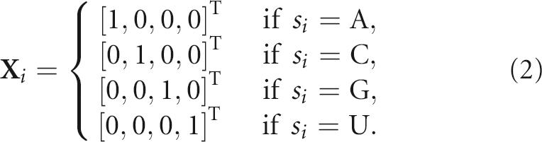The matrix Y represents the sequence pool generated by M with starting sequence S. For example, if

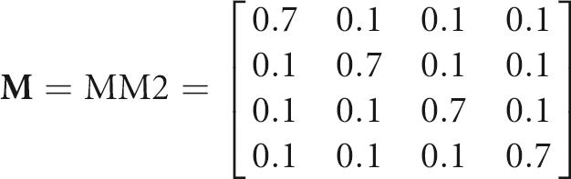and

then Y is given by

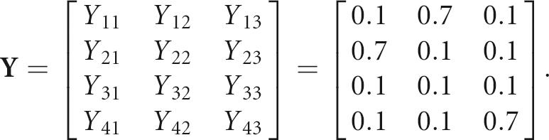The probability of finding a new sequence S′ in the pool can be calculated from Y. For example, P(S′=ACU)=Y ₁₁•Y ₂₂•Y ₄₃=0.1•0.1•0.7 and P(S′=GUC)=Y ₃₁•Y ₄₂•Y ₂₃=0.1•0.1•0.1. Similarly, we can calculate the frequency of sequences with a specified base-pairing scheme using this mathematical formulation. However, a rigorous mapping of sequence space (Y) to shape space (possible RNA graphs) requires an RNA folding algorithm, as described in our previous work (Gan et al. 2003).

The challenge in computational pool design is to find an optimal set of mixing matrix (M), starting sequence (S), and weight (or pool fraction) for generation of target-structured pools. In principle, the mixing matrix can be calculated using statistical thermodynamics from the distribution of shapes in the designed pool. Assuming that the designed pool consists of N noninteracting RNA molecules, the probability of finding topology t in the pool is

where E(S_i) is the energy of sequence S_i, β=1/kT, ρ(E_i) is the density of states, and S _i, β=1/kT, ρ(E _i) is an RNA topology operator defining tree or pseudoknot shapes enumerated by RNA graph theory. Equation (3) defines the relation between sequence pool {S_i} and target structural distribution P(t). Recently, we calculated P(t) distributions for 25–100 nt random pools using a folding algorithm and a program for converting secondary structures into tree graphs (Gevertz et al. 2005). Thus, the goal is to determine the sequence pool {S_i}, or mixing matrices generating that pool, to produce the target distribution P(t). In the Appendix, we describe a practical protocol for finding optimal mixing matrices approximating the target P(t) based on analyses of sequence space and pool structural distribution. Alternative pool design methods may also be developed based on Equation (3).

Pool sizes

For practical reasons, our computations used relatively small pools of 10,000 sequences. To show the effect of pool size, Figure 4 plots the frequency of several tree motifs (4₁, 4₂, 5₁, 5₂, 5₃, and 6₁) for pool sizes of 5,000–60,000 sequences using mixing matrix 4 (MM4) and the initial tRNA sequence. We see that the pool fractions for distinct tree motifs saturate beyond 5000 sequences, indicating that the error due to sample size is small. The rapid saturation of pool fraction stems from mapping secondary structures using simple graphs. If detailed motif features (size of loops, stems, etc.) are incorporated into the mapping, larger pool sizes will certainly be required.

FIGURE 4.

Effect of pool size on pool fractions of selected tree motifs. The pools are generated using random mixing matrix 4 and starting tRNA sequence in Figure 3B.

Measures of sequence and structure similarity

RNA graphs allow global analysis of RNA secondary structures. To analyze sequence and structure space of designed pools at the base level, we use two standard measures of distance between any two RNAs: Hamming distance and tree edit distance. The Hamming distance is the number of differing letters between two equal-length RNA sequences aligned end to end (Hamming 1987). The tree edit distance between two (full) tree secondary structures measures the minimum sum of the cost (insertion, deletion, and replacement of nodes) along an edit path for converting one tree into another (Hofacker 2003). We use the tree edit distance measure as implemented in RNAdistance of the Vienna RNA package available at http://rna.tbi.univie.ac.at. Other distance measures, such as string edit distance or base-pair distance implemented in RNAdistance (Hofacker 2003), can also be used to compare two RNA structures; also available are the more sophisticated sequence/structure alignment algorithms Foldalign (Havgaard et al. 2005) and Dynalign (Mathews and Turner 2002). Here we use Hamming and tree edit distances together with a clustering technique—the multidimensional scaling (MDS) method (Cox and Cox 1994) implemented in the R statistical package (http://www.r-project.org)—to map the RNA sequence/structure space.

RESULTS

Coverage of sequence space regions generated by mixing matrix classes and starting sequences is distinct from random pools

We consider our set of starting sequences (Fig. 3) and 22 mixing matrices (Fig. 2) to explore the sequence/structure space of sequence pools and to optimize target pools.

To analyze the clustering patterns in sequence space, we cluster all sequences generated by the mixing matrices using a standard clustering technique (e.g., MDS), allowing visualization of sequence similarity/dissimilarity properties (Cox and Cox 1994). A similar procedure is commonly used for investigating the diversity of chemical compound libraries (Xie et al. 2000). Such analysis helps establish the relation between each mixing matrix and the generated sequence space. Given a pool of sequences, we define Hamming distances (number of dissimilar bases) between all pairs of sequences (see Materials and Methods), allowing data projections in 2D, 3D, and higher dimensions.

Figure 5, A and B, shows the 2D and 3D clustering of sequences generated by 22 mixing matrices using starting sequences for the modified P5abc (Fig. 3E) and 70S (Fig. 3A) RNAs, respectively. In Figure 5A, we see that the sequences generated by the five mixing matrix classes and the P5abc starting sequence cover distinct regions of the sequence space, especially the boundary and central regions. The boundaries are spanned by matrix classes B–E, and the central region by matrix class A. Intriguingly, the random MM4 produces sequences that are localized in sequence space, showing that the standard approach does not provide an efficient sampling of diverse regions of sequence space in agreement with observations. More adequate sampling of sequence space is provided by the nonrandom mixing matrices. The 70S starting sequence yields similar global 2D and 3D clustering patterns: the five matrix classes yield clusters in distinct sequence regions (Fig. 5B). Although the 22 mixing matrices of Figure 2 provide a comprehensive coverage of the sequence space, some regions remain sparsely populated, indicating that the matrix classes must be expanded for more complete coverage. Still, the chosen matrix set is diverse enough for initial assessment of our structured pool design concept.

FIGURE 5.

Two- and three-dimensional clustering plots using the MDS transformation for sequences generated from 22 mixing matrices (labeled 1–22) (A) starting with a modified P5abc domain (Fig. 3E) and (B) with 70S (Chain F) (Fig. 3A). The distance between any sequence pair is the Hamming distance, a measure of the number of dissimilar nucleotide bases. Axes represent two or three largest components of the projection. Each color represents a sequence pool generated by one of the 22 mixing matrices; the “×” mark on the left represents result for an invariant sequence transformation corresponding to diagonal matrix M _ii=1. The mixing matrices are grouped into five classes (A–E) according to their matrix properties (Table 1).

RNA motif distributions depend on generating mixing matrices

By “folding” the resulting pool sequences using Vienna RNAfold and converting motifs into tree graphs, we can assess each pool's structural distribution (Gan et al. 2003; Gevertz et al. 2005). Figure 6 shows the frequencies of various tree motifs in pools generated by the 22 mixing matrices starting with the 4₂ tree motif from the modified P5abc (Fig. 3E). Corresponding distributions for all six starting sequences in Figure 3 are shown in Table 2. In Table 2, populations of <0.5% are reported as 0.

FIGURE 6.

Pool fraction distributions for six tree motifs in pools generated from 22 mixing matrices (labeled 1–22), starting with a modified P5abc domain (Fig. 3E), which has a 4₂ tree motif. The results for the random pool 4 (marked with arrow) are displayed as dot-filled histograms.

TABLE 2.

Structural distributions of pools generated by 22 mixing matrices in Figure 2 starting with the six sequences in Figure 3, A–F

First, it is evident that motif distributions in our designed pools vary significantly from those in random pools (MM4; see arrow and dot-filled histograms). For example, with the Figure 3E starting sequence, the 4₂ tree motif has a yield of ∼8%, for the random mixing matrix, versus 79%, 46%, and 34% in matrix pools 7–9, which do not mutate C and G bases, respectively. At the other extreme, matrices 20–22 produce small proportions (5%–6%) of 4₂ tree structure. For the 3₁ tree motif, mixing matrices 5, 6, 14, 15, 19, 20, 21, and 22 generate higher pool fractions than the random pool 4, whereas matrices 7–13 yield considerably lower numbers. Thus, motif distributions depend on both the mixing matrix and the starting sequence because different sequence space regions result. Because the overlap of sequence regions of our 22 pools is weak, the motif distribution is very different in each case (Fig. 5).

Second, we note a pattern in the correlation between 4₂ and 5₂ trees and between 3₁ and 4₁ trees. With the Figure 3E starting sequence, Figure 6 and Table 2 show that sequence pools from matrices 7–13 have a large proportion of 4₂ and 5₂ tree structures compared with the random pool 4. Similarly pools from matrices 14–22 possess >30% 3₁ and 4₁ tree structures. This pattern emerges because the 4₂/5₂ and 3₁/4₁ tree-motif pairs are related by an internal loop or bulge, which can be created by a few mismatched base pairs.

Third, the structural distributions generated by a tRNA sequence (5₃ tree motif; Fig. 3B) differ from those for the modified P5abc domain (4₂ tree motif; Fig. 3E) in one important respect (Table 2). The most likely motifs are the simpler 5₁ and 5₂ trees rather than the starting 5₃ motif. MM1, for example, generates only 5% 5₃ motif, but 26% 5₂ tree. In contrast, MM7, which preserves C and G bases, generates 23% 5₃ trees, while other combinations of mixing matrices and starting structures yield almost no 5₃ trees (Table 2). The mean mutation rate for MM7 from the starting tRNA sequence (Fig. 3B) is ∼0.1 (∼8.5 positions among 81 nt). Thus, the 5₃ motif populations produced by matrices 1 and 7–11 are much higher than in random pools (1.3%). The difficulty of generating significant populations with the tRNA-like 5₃ tree motif likely stems from the lower thermodynamic stability of 5₃ compared to 5₁ and 5₂ trees. Our analysis shows that matrices 7–9 generate sequences that are favorable for stabilizing the 5₃ motif because these matrices preserve energetically favorable CG base pairs.

To increase the population of complex folds like the tRNA-like 5₃ tree motif, we consider refining the mixing matrices 7–9. Since class B matrices 7–9 produce a higher frequency of 5₃ tree, we search for matrices in the neighborhood of this class by exhaustively varying the elements in each row with ΔM _ij=0.2, yielding 56 possible cases. Assuming that each row is independent, the total number of mixing matrices around the class B matrix region is 56² or 3136, since two rows (second and third) are identical and the other two rows (first and last) have a total of 56 cases each. We filter the 3136 trial mixing matrices, yielding better than a 23% tRNA-like 5₃ tree structure. Remarkably, 12 of the 3136 mixing matrices for tRNA-like topology fulfill our requirement forming 5₃ motifs. We use these “MMT” matrices (Fig. 7) to generate graph-structural distributions with tRNA shapes, as shown in Table 3. For example, MMT6 generates a 51% tRNA-like 5₃ tree motif with 15 mutations out of 81 bases.

FIGURE 7.

Twelve refined or variants of class B mixing matrices for enhancing pools with the tRNA-like (5₃) structure (MMT); they generate pools with at least 23% 5₃ tree motif.

TABLE 3.

Structural distributions of pools generated by 12 refined class B mixing matrices in Figure 7 starting with the tRNA sequence in Figure 3B

Note that each pool generated by the 12 mixing matrices has 5000 sequences. Compared with the random pool, these refined matrices generate complex structures (e.g., 5₃ and also 6₄ and 6₅) routinely. This search demonstrates the feasibility of improving yields of specific structures using appropriate mixing matrices and starting sequences.

Sequence/structure correlations exist in designed pools

The above survey of tree structural distributions provides an analysis of RNA shapes in designed pools. We now analyze sequence/structure distributions at the nucleotide base level generated by the 22 mixing matrices starting with a 51-nt P5abc domain (Fig. 3E). In Figure 8, we use sequence Hamming and tree edit distances to quantify sequence and structure distances, respectively, as defined in Materials and Methods. Recall that the Hamming distance is the number of differing letters between two equal-length RNA sequences aligned end to end (Hamming 1987). The tree edit distance between two (full) tree secondary structures measures the minimum sum of the cost (insertion, deletion, and replacement of nodes) along an edit path for converting one tree into another (Hofacker 2003).

FIGURE 8.

Contour plots of sequence/structure relationships using Hamming distance versus tree edit distance for pools generated by 22 mixing matrices, starting from a modified P5abc domain (Fig. 3E). Note that the X and the Y axes are always 0–100 and 0–60, respectively, and that each intensity bar indicates the frequency of joint distance distributions (the frequency outside the box is 0). There are 10,000 sequences in each pool.

All mixing matrices give rise to localized distributions as measured from the initial sequence/structure. As the matrix diagonal elements decrease from 0.85 to 0 (class A matrices 1–6), both sequence and structure distances increase. The sequence distance is determined by the strength of the nondiagonal elements, with matrices 1 and 6 yielding the smallest and largest Hamming distances, respectively. As expected, classes B (7–10) and C (11–14) with fixed C, G and A, U, respectively, produce distributions with small Hamming distances. In contrast, classes D (15–17) and E (19–21) produce sequences with the maximum Hamming distance because no identity base transition is allowed.

As the mixing matrices are altered, the distribution of the tree edit distances also changes. Generally, tree edit distance increases with mutation rate. For example, Figure 8 shows that tree edit distances become larger as diagonal elements of matrix classes A, B, and C decrease. Changing C and G bases (matrix class C) has a larger effect on the starting structure than changing A and U bases (matrix class B), as evident from the pool distances from the origin. This is due to lower free energies associated with GC base pairs compared to AU base pairs. Thus, Figure 8 indicates that the distribution of sequence/structure distances from the initial sequence is controlled by the elements of the mixing matrices. Although the patterns of sequence/structure distributions are not sensitive to the starting sequences (data not shown), the densities within the localized regions are markedly changed. Figure 8 shows that the pools generated by most mixing matrices (except for 1, 8, and 9) and starting sequences of a modified P5abc domain produce a single cluster. We find that contour plots with string edit distance or base-pair distance (data not shown) show somewhat less information about pool structural properties than those with tree edit distance. Other secondary structure measures may also be used to capture structural differences among folds in the same vertex or tree class. For example, it is informative to know the distribution of stem, loop, and bulge sizes (Fontana et al. 1993).

Parameter optimization can lead to design of structured RNA pools

The preceding analysis of sequence space and assessment of structural distributions generated by nonrandom mixing matrices allow design of target structured pools. Here we use the pool design algorithm (Appendix) to develop several structured pools by selecting an optimal combination of starting sequences, mixing matrices, and associated weights {(S_i, M _i, α_i)}. The best combination for a target pool is dictated by the frequency data (Fig. 6; Tables 2, 3).

To illustrate, Table 4 shows four examples of designed pools that are rich in specific tree structures (e.g., 4₁, 5₁, 5₂); also displayed are their pool characteristics (mixing matrix weights and tree motif frequencies). Specifically, our target pools are: Pool T_A with 4₁ and 4₂ structures; Pool T_B with 5₁, 5₂, and 5₃ structures; Pool T_C with 4₂, 5₂, and 5₃ structures; and Pool T_D with 4₁, 4₂, and 5₃ structures. Pools T_A and T_B are 4- and 5-vertex pools, respectively, and Pools T_C and T_D are pools with mixed n-vertex structures. Each designed pool represents an optimal combination of starting sequences, mixing matrices, and associated weights derived using Step 5 of our design algorithm (see Appendix). Briefly, we initially choose pool fractions T ₁, T ₂, …, T_n for target motifs and the number of mixing matrices to approximate the target pool. We then use Equation (6) in the Appendix to calculate the weight α₁, which depends on T ₁, starting sequence S ₁, and mixing matrix M ₁. Next, we minimize the error between the target and estimated target pool fractions, Equation (8) in the Appendix, over all pools generated by starting sequence/mixing matrix pairs {(S_i, M _i)}. This procedure yields optimized starting sequences, mixing matrices, and weights; the mean mutation rate is calculated based on these sequences, mixing matrices, and their weights.

TABLE 4.

Five designed structured pools (T_A–T_E) and their characteristics

As shown in Table 4, the optimized Pool T_A for a 30% 4₂ tree (T ₁) and for a 25% 4₁ structure (T ₂) is constructed using the Figure 3E starting sequence for matrices 8 and 3 with weights of 0.556 and 0.444, respectively. The mean mutation rate is 0.337 compared to the random base mutation rate of 0.75. Correspondingly, our designed pool for 4₁ and 4₂ motifs contains 25% and 30% 4₁ and 4₂ trees, respectively, compared with 29% and 12% for the random pool (MM4). The increase of 4₂ species is accompanied by the decrease of the 5₁ structure to 6% compared with 23% for the random Pool T_F. The next highest species in Pool T_A is 3₁ (22%).

Pool T_B, targeting 20% each of the 5₁, 5₂, and 5₃ structures, is generated from the Figure 3A sequence for 5₁ with matrix 13 at a weight of 0.18 and the Figure 3B sequence for 5₃ with matrix T12 at a weight of 0.82. For this pool optimization, we expanded our mixing matrix/starting sequence repertoire to include those in Table 3 (the 12 mixing matrices for generating pools with a high frequency of 5₃ motifs, which are extremely rare in random pools). Thus, this optimization was performed over the set of 144 (22×6+12×1) mixing matrix/starting sequence pairs.

Resulting Pool T_B contains 20% each 5₁, 5₂, and 5₃ tree motifs, compared with 23%, 16%, and 0% for the random pool (MM4), matching the target exactly. We found that using the 12 MMT matrices dramatically increases the population of the 5₃ motif (at a cost of decrease of 3₁, 4₁, and 4₂ motifs). The 6₁ structure (9%) is the next highest species in Pool T_B.

Target Pools T_C and T_D are mixed pools with both 4- and 5-vertex tree structures, designed from our 144 mixing matrix/starting sequence pairs. The targets for Pool T_C are 4₂, 5₂, and 5₃ tree motifs, and those for Pool T_D are 4₁, 4₂, and 5₃ tree motifs (20% for each). Pool T_C is generated by the Figure 3E sequence (MM9, 0.60) and the Figure 3B sequence (MMT2, 0.40), and Pool T_D is produced by the Figure 3B sequence (MMT6, 0.329) and the Figure 3F sequence (MM13, 0.608). The results are as expected: Pool T_C has frequencies for 4₂, 5₂, and 5₃ motifs of between 19% and 20%; Pool T_D has frequencies for 4₁, 4₂, and 5₃ trees of 17%, 20%, and 20%, respectively, all within 3% of the target.

Our designed pools above, involving three of the 22 mixing matrices and two of the 12 MMT matrices, only touched the surface of possibilities. Still, in practice, it might be preferable to approximate a target pool using a small number of mixing matrices. Once our algorithm is automated (Appendix), exploration of pool design can be routinely performed.

A designed pool improves the selection of GTP aptamers

We now apply our pool design approach for enhancing GTP-binding aptamers. Szostak's group recently found that the GTP aptamer's binding affinity is correlated with the informational complexity (Carothers et al. 2004, 2006). Informational complexity is correlated with structural complexity (e.g., number of stems, vertex number of tree graph). As the information content and binding affinity decrease (Carothers et al. 2004, see their Fig. 1, panels A and B), the aptamers have simple structures such as 2₁ or 3₁ tree motifs. Specifically, a high-affinity GTP aptamer with high informational complexity (Carothers et al. 2004, see their Fig.1, panel C) has the 5₂ tree structure (Fig. 3D). Interestingly, no GTP aptamer with a 4₂ tree structure (Fig. 3F) has been reported, although it is structurally similar to the 5₂ tree. Because the frequency of the 4₂ motif is only 12% in the random Pool T_F (Table 4), we propose designing a GTP aptamer pool by enriching the pool with 5₂ and 4₂ motifs. Our target pool fractions (T_i) are 20% for 4₂ and 26% for 5₂. Our optimization yields Pool T_E (Table 4) as a combination of two subpools: the Figure 3D sequence (MM13, 0.625) and the Figure 3F sequence (MM10, 0.375). The frequencies of 4₂ and 5₂ trees in the designed pool are 21% and 26%, respectively, nearly as desired and very different for the 12% and 16% distributions of these motifs in the random Pool T_F. The sequence/structure contour plots in Figure 9 show differences between the designed and random pools; the designed pool has a relatively high mean mutation rate of 0.349.

FIGURE 9.

Comparison of designed GTP (upper) and random (lower) pools using contour plots of Hamming distance versus tree edit distance. The GTP pool is generated by 62.5% MM13 starting with the 5₂ motif (Fig. 3D) and 37.5% MM10 starting with the 4₂ motif (Fig. 3F). The random pool is generated using the starting sequence in Figure 3D.

DISCUSSION

Following our previous analysis that random RNA pools are not structurally diverse (Gevertz et al. 2005), we have proposed computational tools for designing RNA pools for enhancing in vitro selection based on sequence/structure relationships. We represent pool synthesis experiments as mixing matrices applied to starting sequences; this approach can be likened to considering mutations around given sequences. Such mutations are then optimized to target specific structures and increase structural diversity. By constructing five classes of mixing matrices based mainly on conservation of base pairs, we have developed 22 representative mixing matrices covering diverse regions of the sequence space. We showed that sequence diversity represented by the mixing matrices leads to greater structural diversity, allowing the design of pools with target structural characteristics through optimization of starting sequence/mixing matrix pairs and associated weights (pool fraction for each pair). The optimized mixing matrix/starting sequence pairs and weights provide sufficient information for pool synthesis.

Thus, our work suggests that designing pools for enhancing in vitro selection can follow several research avenues. Maximizing sequence and structural diversity broadly can increase the probability of finding a given RNA property using nonrandom mixing matrix/starting sequence pairs. An advantage of this approach is that designed pools can be directly implemented in pool synthesis. Alternatively, we can target a specific structural distribution by determining optimal mixing matrices and starting sequences without explicit sequence/structure mapping. Our targeted pool design can be applied to known structures, novel motifs (Kim et al. 2004), complete sets like n-vertex pools, or perhaps submotifs of RNAs (Zorn et al. 2004). Of course, a more comprehensive set of mixing matrices covering wider regions of the sequence space should be sought systematically. For example, matrices conserving noncanonical base pairs (AC, CA, GA, AG, etc.) can complement our current set, which conserves canonical base pairs; there are 12 such classes from a total of 16 possible base pairs.

Another design theme is enrichment of pools with structures resembling a target-active molecule. We illustrated this approach using GTP-binding aptamers. The conventional approach – designing pools in the sequence neighborhood of a target molecule (Lau et al. 2004; Ohuchi et al. 2004; Yoshioka et al. 2004), however, does not ensure that the designed pools will cover the structural neighbors of the target molecule, unless sequence mutations are made to localized sequence segments, as is commonly done in many experiments. In contrast, our optimized pool design approach (Appendix), allows enrichment of pools with specific RNA topologies or structures (e.g., tRNA-like 5₃ tree). In addition, novel tree topologies in the neighborhood of the target molecule, as suggested by structural enumeration (Kim et al. 2004), could be similarly engineered.

Clearly, further developments of sequence/structure analysis techniques are needed to improve the pool design and overcome specific limitations. Understanding the sequence/structure relationship is one of the most fundamental biological problems not only for RNA but also for proteins. In our analysis, we are limited by the usage of numerical secondary structure folding algorithms, which are still imperfect and inefficient for predicting pseudoknot structures. However, our risk has been reduced here by “folding” of small RNAs (<100 nt) only and focusing on statistical properties (e.g., frequencies of topologies). A general strategy for improving structure prediction is to consider many suboptimal structures using, for example, the Boltzmann sampling method (Ding and Lawrence 2003).

Ultimately, RNA tertiary and higher-order folding is essential to understand RNA function. Perhaps progress on this problem will be realized in the near future. For now, we offer our sequence pools possessing diverse RNA secondary structures as an approach to enhance in vitro selection technology.

Our pool design algorithm can be fully automated given target RNA shapes (and possibly starting sequences). We are developing a publicly available Web server to allow experimentation of pool design and analysis of RNA pool properties (e.g., base composition, size distribution of stems, bulges, etc.), and to define optimal mixing matrices for pool synthesis. Experimental synthesis of designed pools (specific structural motifs and their frequency) can be performed by using optimized starting sequences, mixing matrices, and associated weights. When available, location of this server will be noted on our group Web site (http://monod.biomath.nyu.edu). We hope that this tool will help stimulate the productive interaction between theoretical and experimental efforts.

APPENDIX

An algorithm for designing structured RNA pools

Our pool design algorithm is based on analyses of sequence and structure spaces to allow design of specific structures, including novel RNA-like motifs identified using graph theory analysis (Kim et al. 2004). The algorithm below assumes that we have available reference data such as shown in Tables 2 and 3 that relate mixing matrices and starting sequences to motif distributions in resulting pools. The sequence space regions are mapped via various mixing matrices using a standard clustering method; the structural distribution is computed by converting secondary structures into tree graphs. By knowing the structural distributions of various sequence space regions, we then can optimize the choice of starting sequences and mixing matrices to approximate the target structured pool for future work.

Our pool design algorithm involves the following steps:

1. Specify a target distribution of topologies/shapes.

2. Define candidates for starting sequences and mixing matrices that aim to cover the sequence space. The mixing matrices have been constructed, for example, based on covariance mutations. The mixing matrices and starting sequences may remain the same for different structured pool designs. We “visualize” the diversity of a set of RNA sequences using a standard sequence similarity/dissimilarity clustering based on Hamming distance (number of dissimilar bases) between any pair of aligned sequences. In this study, we used mainly six starting sequences and constructed 22 mixing matrices to cover the sequence space (see Results).

3. Compute shape frequency distributions corresponding to all starting sequence/mixing matrix pairs, as discussed below and detailed in our previous study (Gevertz et al. 2005). This step analyzes pool structural diversity.

4. Choose the number of mixing matrices to approximate the designed pool.

5. Find an optimal combination of starting sequences (S_i) and mixing matrices (M _i) and associated weights (α_i) to approximate the target RNA shape distribution. The mathematical procedures for this step are detailed below.

The designed pool is composed of k smaller subpools defined by the set {(S_i, M _i, α_i)}, i=1, 2, …, k. The above pool design algorithm can be fully automated given target RNA shapes (and possibly starting sequences). We are planning to make publicly available a Web server to allow experimentation of pool design and analysis of RNA pool properties, and to obtain mixing matrices for pool synthesis. Experimental synthesis of designed pools can be performed by using trial S_i, M _i, and α_i.

In Step 3, the pool structural distribution is calculated by mapping RNA secondary structures into graph space. This is done by predicting secondary structures of all sequences using the Vienna RNAfold package and then converting them into tree graphs, as described elsewhere (Gevertz et al. 2005). It is known that 73% of known base pairs are predicted by free-energy minimization algorithms such as RNAfold for sequences with <700 nt (Mathews and Turner 2006). For greater accuracy, the Boltzmann sampling method can be used to generate a set of 1000 suboptimal structures (Ding and Lawrence 2003), although at a higher computational cost (1000 times pool size). Specifically, base-pairing information in the .ct file generated by the RNAfold program is used to convert a secondary fold into a tree graph. The topologies of the folds are determined using Laplacian eigenvalues of tree graphs as implemented in our RNA Matrix Program (Gan et al. 2004) (server available at http://monod.biomath.nyu.edu/rna). Specifying tree topologies using eigenvalues is inexact because different topologies can have the same spectrum; the assignment error rate is a few percent for small tree topologies (<10 vertices). This step is similar to the RNAshapes program, which uses bracket notations for representing secondary structures (Giegerich et al. 2004; Steffen et al. 2006). Unless stated otherwise, each sequence pool has 10,000 sequences, which is adequate for assessing structural distributions using simple tree graphs. Structure prediction and conversion to tree graphs for 10,000 80-nt sequences require ∼1 h on an SGI 300 MHz MIPS R12000 IP27 processor.

In Step 5, we approximate a target structural distribution by optimizing a set of starting sequence/mixing matrix pairs based on pool structural frequency data. Generally, we consider a designed pool composed of k subpools, each generated with a mixing matrix/starting sequence pair and associated with a weight α_i: p(S ₁, M ₁, α₁), p(S ₂, M ₂, α₂), …, p(S_k, M _k, α_k), where α₁+α₂+…+α_k=1 and p(S_i, M _i, α_i) denotes synthesizing the α_i fraction of the pool sequences using starting sequence S_i and mixing matrix M _i. Optimization of the three pool parameters S_i, M _i, and α_i can be formulated as follows: If the n×1 matrix T is the target distribution with T_i fractions of structures 1, 2, …, n and F_l(S_i, M _i) is the pool fraction of structure l generated by starting sequence S_i and mixing matrix M _i in Tables 2 and 3, the pool parameters (S_i, M _i, α_i) can be optimized by the following equation:

where α=(α_1, α_2, …, α_k) subject to the conditions α₁+α₂+…+α_k=1 and α_i≥0. Since experimental implementation of pool synthesis is simpler with fewer mixing matrices, we consider the solution of α for k=2 below; the optimization procedure can be generalized. Formula (4) with only two mixing matrices M ₁ and M ₂ reduces to

The solution for the only weight is

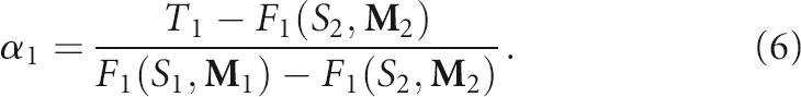The estimated pool fractions for the other shapes or topologies 2, 3, …, n are derived from the known α₁, F ₁(S ₁, M ₁), and F ₁(S ₂, M ₂) as follows:

We then optimize (S ₁, M ₁), and (S ₂, M ₂) by minimizing the error

The above procedure will allow us to obtain the optimized parameters α₁, (S ₁, M ₁), and (S ₂, M ₂) for a target distribution T. The convergence of the procedure depends on the number of mixing matrices and starting sequences, or coverage of the sequence/structure space.

REFERENCES

- Breaker, R.R. Natural and engineered nucleic acids as tools to explore biology. Nature. 2004;432:838–845. doi: 10.1038/nature03195. [DOI] [PubMed] [Google Scholar]
- Carothers, J.M., Oestreich, S.C., Davis, J.H., Szostak, J.W. Informational complexity and functional activity of RNA structures. J. Am. Chem. Soc. 2004;126:5130–5137. doi: 10.1021/ja031504a. [DOI] [PMC free article] [PubMed] [Google Scholar]
- Carothers, J.M., Davis, J.H., Chou, J.J., Szostak, J.W. Solution structure of an informationally complex high-affinity RNA aptamer to GTP. RNA. 2006;12:567–579. doi: 10.1261/rna.2251306. [DOI] [PMC free article] [PubMed] [Google Scholar]
- Cox, T.F., Cox, M.A.A. Multidimensional scaling. Chapman & Hall; Boca Raton, FL: 1994. [Google Scholar]
- Davis, J.H., Szostak, J.W. Isolation of high-affinity GTP aptamers from partially structured RNA libraries. Proc. Natl. Acad. Sci. 2002;99:11616–11621. doi: 10.1073/pnas.182095699. [DOI] [PMC free article] [PubMed] [Google Scholar]
- Ding, Y., Lawrence, C.E. A statistical sampling algorithm for RNA secondary structure prediction. Nucleic Acids Res. 2003;31:7280–7301. doi: 10.1093/nar/gkg938. [DOI] [PMC free article] [PubMed] [Google Scholar]
- Eddy, S.R., Durbin, R. RNA sequence analysis using covariance models. Nucleic Acids Res. 1994;22:2079–2088. doi: 10.1093/nar/22.11.2079. [DOI] [PMC free article] [PubMed] [Google Scholar]
- Ellington, A.D., Szostak, J.W. In vitro selection of RNA molecules that bind specific ligands. Nature. 1990;346:818–822. doi: 10.1038/346818a0. [DOI] [PubMed] [Google Scholar]
- Famulok, M., Verma, S. In vivo applied functional RNAs as tools in proteomics and genomics research. Trends Biotechnol. 2002;20:462–466. doi: 10.1016/s0167-7799(02)02063-2. [DOI] [PubMed] [Google Scholar]
- Fera, D., Kim, N., Shiffeldrim, N., Zorn, J., Laserson, U., Gan, H.H., Schlick, T. RAG: RNA-As-Graphs web resource. BMC Bioinformatics. 2004;5:88–96. doi: 10.1186/1471-2105-5-88. [DOI] [PMC free article] [PubMed] [Google Scholar]
- Fontana, W., Konings, D.A.M., Stadler, P.F., Schuster, P. Statistics of RNA secondary structures. Biopolymers. 1993;33:1389–1404. doi: 10.1002/bip.360330909. [DOI] [PubMed] [Google Scholar]
- Gan, H.H., Pasquali, S., Schlick, T. Exploring the repertoire of RNA secondary motifs using graph theory; implications for RNA design. Nucleic Acids Res. 2003;31:2926–2943. doi: 10.1093/nar/gkg365. [DOI] [PMC free article] [PubMed] [Google Scholar]
- Gan, H.H., Fera, D., Zorn, J., Shiffeldrim, N., Tang, M., Laserson, U., Kim, N., Schlick, T. RAG: RNA-As-Graphs database—Concepts, analysis, and features. Bioinformatics. 2004;20:1285–1291. doi: 10.1093/bioinformatics/bth084. [DOI] [PubMed] [Google Scholar]
- Gevertz, J., Gan, H.H., Schlick, T. In vitro RNA random pools are not structurally diverse: A computational analysis. RNA. 2005;11:853–863. doi: 10.1261/rna.7271405. [DOI] [PMC free article] [PubMed] [Google Scholar]
- Giegerich, R., Voss, B., Rehmsmeier, M. Abstract shapes of RNA. Nucleic Acids Res. 2004;32:4843–4851. doi: 10.1093/nar/gkh779. [DOI] [PMC free article] [PubMed] [Google Scholar]
- Hamming, R.W. Coding and information theory. Prentice-Hall; Englewood Cliffs, NJ: 1987. [Google Scholar]
- Havgaard, J.H., Lyngso, R.B., Gorodkin, J. The FOLDALIGN web server for pairwise structural RNA alignment and mutual motif search. Nucleic Acids Res. 2005;33:W650–W653. doi: 10.1093/nar/gki473. [DOI] [PMC free article] [PubMed] [Google Scholar]
- Hermann, T., Patel, D.J. Biochemistry—Adaptive recognition by nucleic acid aptamers. Science. 2000;287:820–825. doi: 10.1126/science.287.5454.820. [DOI] [PubMed] [Google Scholar]
- Hofacker, I.L. Vienna RNA secondary structure server. Nucleic Acids Res. 2003;31:3429–3431. doi: 10.1093/nar/gkg599. [DOI] [PMC free article] [PubMed] [Google Scholar]
- Isaacs, F.J., Dwyer, D.J., Collins, J.J. RNA synthetic biology. Nat. Biotechnol. 2006;24:545–554. doi: 10.1038/nbt1208. [DOI] [PubMed] [Google Scholar]
- Jaeger, L., Wright, M.C., Joyce, G.F. A complex ligase ribozyme evolved in vitro from a group I ribozyme domain. Proc. Natl. Acad. Sci. 1999;96:14712–14717. doi: 10.1073/pnas.96.26.14712. [DOI] [PMC free article] [PubMed] [Google Scholar]
- Jäschke, A. Artificial ribozymes and deoxyribozymes. Curr. Opin. Struct. Biol. 2001;11:321–326. doi: 10.1016/s0959-440x(00)00208-6. [DOI] [PubMed] [Google Scholar]
- Kim, N., Shiffeldrim, N., Gan, H.H., Schlick, T. Candidates for novel RNA topologies. J. Mol. Biol. 2004;341:1129–1144. doi: 10.1016/j.jmb.2004.06.054. [DOI] [PubMed] [Google Scholar]
- Knight, R., De Sterck, H., Markel, R., Smit, S., Oshmyansky, A., Yarus, M. Abundance of correctly folded RNA motifs in sequence space, calculated on computational grids. Nucleic Acids Res. 2005;33:5924–5935. doi: 10.1093/nar/gki886. [DOI] [PMC free article] [PubMed] [Google Scholar]
- Lau, M.W., Cadieux, K.E., Unrau, P.J. Isolation of fast purine nucleotide synthase ribozymes. J. Am. Chem. Soc. 2004;126:15686–15693. doi: 10.1021/ja045387a. [DOI] [PubMed] [Google Scholar]
- Lee, J.F., Hesselberth, J.R., Meyers, L.A., Ellington, A.D. Aptamer database. Nucleic Acids Res. 2004;32:D95–D100. doi: 10.1093/nar/gkh094. [DOI] [PMC free article] [PubMed] [Google Scholar]
- Legiewicz, M., Lozupone, C., Knight, R., Yarus, M. Size, constant sequences, and optimal selection. RNA. 2006;11:1701–1709. doi: 10.1261/rna.2161305. [DOI] [PMC free article] [PubMed] [Google Scholar]
- Mathews, D.H., Turner, D.H. Dynalign: An algorithm for finding the secondary structure common to two RNA sequences. J. Mol. Biol. 2002;317:191–203. doi: 10.1006/jmbi.2001.5351. [DOI] [PubMed] [Google Scholar]
- Mathews, D.H., Turner, D.H. Prediction of RNA secondary structure by free-energy minimization. Curr. Opin. Struct. Biol. 2006;16:270–278. doi: 10.1016/j.sbi.2006.05.010. [DOI] [PubMed] [Google Scholar]
- Ohuchi, S.J., Ikawa, Y., Shiraishi, H., Inoue, T. Modular engineering of a Group I intron ribozyme. Nucleic Acids Res. 2002;30:3473–3480. doi: 10.1093/nar/gkf453. [DOI] [PMC free article] [PubMed] [Google Scholar]
- Ohuchi, S.J., Ikawa, Y., Shiraishi, H., Inoue, T. Artificial modules for enhancing rate constants of a Group I intron ribozyme without a P4-P6 core element. J. Biol. Chem. 2004;279:540–546. doi: 10.1074/jbc.M305499200. [DOI] [PubMed] [Google Scholar]
- Ren, J.H., Rastegari, B., Condon, A., Hoos, H.H. HotKnots: Heuristic prediction of RNA secondary structures including pseudoknots. RNA. 2005;11:1494–1504. doi: 10.1261/rna.7284905. [DOI] [PMC free article] [PubMed] [Google Scholar]
- Rivas, E., Eddy, S.R. A dynamic programming algorithm for RNA structure prediction including pseudoknots. J. Mol. Biol. 1999;285:2053–2068. doi: 10.1006/jmbi.1998.2436. [DOI] [PubMed] [Google Scholar]
- Schultes, E., Hraber, P.T., LaBean, T.H. Global similarities in nucleotide base composition among disparate functional classes of single-stranded RNA imply adaptive evolutionary convergence. RNA. 1997;3:792–806. [PMC free article] [PubMed] [Google Scholar]
- Soukup, G.A., Breaker, R.R. Engineering precision RNA molecular switches. Proc. Natl. Acad. Sci. 1999a;96:3584–3589. doi: 10.1073/pnas.96.7.3584. [DOI] [PMC free article] [PubMed] [Google Scholar]
- Soukup, G.A., Breaker, R.R. Nucleic acid molecular switches. Trends Biotechnol. 1999b;17:469–476. doi: 10.1016/s0167-7799(99)01383-9. [DOI] [PubMed] [Google Scholar]
- Soukup, G.A., Breaker, R.R. Allosteric nucleic acid catalysts. Curr. Opin. Struct. Biol. 2000;10:318–325. doi: 10.1016/s0959-440x(00)00090-7. [DOI] [PubMed] [Google Scholar]
- Steffen, P., Voss, B., Rehmsmeier, M., Reeder, J., Giegerich, R. RNAshapes: An integrated RNA analysis package based on abstract shapes. Bioinformatics. 2006;22:500–503. doi: 10.1093/bioinformatics/btk010. [DOI] [PubMed] [Google Scholar]
- Storz, G. An expanding universe of noncoding RNAs. Science. 2002;296:1260–1263. doi: 10.1126/science.1072249. [DOI] [PubMed] [Google Scholar]
- Stuhlmann, F., Jäschke, A. Characterization of an RNA active site: Interactions between a Diels–Alderase ribozyme and its substrates and products. J. Am. Chem. Soc. 2002;124:3238–3244. doi: 10.1021/ja0167405. [DOI] [PubMed] [Google Scholar]
- Tuerk, C., Gold, L. Systematic evolution of ligands by exponential enrichment: RNA ligands to bacteriophage T4 DNA polymerase. Science. 1990;249:505–510. doi: 10.1126/science.2200121. [DOI] [PubMed] [Google Scholar]
- Wilson, D.S., Szostak, J.W. In vitro selection of functional nucleic acids. Annu. Rev. Biochem. 1999;68:611–647. doi: 10.1146/annurev.biochem.68.1.611. [DOI] [PubMed] [Google Scholar]
- Xie, D.X., Tropsha, A., Schlick, T. An efficient projection protocol for chemical databases: Singular value decomposition combined with truncated-Newton minimization. J. Chem. Inf. Comput. Sci. 2000;40:167–177. doi: 10.1021/ci990333j. [DOI] [PubMed] [Google Scholar]
- Yoshioka, W., Ikawa, Y., Jaeger, L., Shiraishi, H., Inoue, T. Generation of a catalytic module on a self-folding RNA. RNA. 2004;10:1900–1906. doi: 10.1261/rna.7170304. [DOI] [PMC free article] [PubMed] [Google Scholar]
- Zorn, J., Gan, H.H., Shiffeldrim, N., Schlick, T. Structural motifs in ribosomal RNAs: Implications for RNA design and genomics. Biopolymers. 2004;73:340–347. doi: 10.1002/bip.10525. [DOI] [PubMed] [Google Scholar]