Local Effects of Delayed Food

Abstract

Five pigeons were trained on a procedure in which seven concurrent variable-interval schedules arranged seven different food–rate ratios in random sequence in each session. Each of these components lasted for 10 response-produced food deliveries, and components were separated by 10-s blackouts. We varied delays to food (signaled by blackout) between the two response alternatives in an experiment with three phases: In Phase 1, the delay on one alternative was 0 s, and the other was varied between 0 and 8 s; in Phase 2, both delays were equal and were varied from 0 to 4 s; in Phase 3, the two delays summed to 8 s, and each was varied from 1 to 7 s. The results showed that increasing delay affected local choice, measured by a pulse in preference, in the same way as decreasing magnitude, but we found also that increasing the delay at the other alternative increased local preference. This result casts doubt on the traditional view that a reinforcer strengthens a response depending only on the reinforcer's value discounted by any response–reinforcer delay. The results suggest that food guides, rather than strengthens, behavior.

In the view of 19th- and 20th-century associationism, which made contiguity between events paramount, a delay between two events would singularly diminish their connection. This thinking was carried over to the law of effect, with the result that Thorndike and many who came after him tried to overcome the problem of action at a distance with special explanations for the effects of delay of reinforcement (Kimble, 1961). In contrast, some authors have suggested that reinforcer delay might be treated as just another payoff parameter, similar but opposite in effect to reinforcer magnitude (Kimble, 1961). Since the discovery of the matching law (Herrnstein, 1961) and its generalization (Baum, 1974), several authors have suggested that delay, or its reciprocal immediacy, might be incorporated into a concatenated version of matching in the same way as rate and magnitude (Baum & Rachlin, 1969; Killeen, 1972; Rachlin, 1971). The equation is:

1

where B_L/B_R is the response ratio between food deliveries, R_L/R_R is the ratio of obtained food rates (which is usually close to the arranged ratio), M_L/M_R is the magnitude ratio, and I_L/I_R is the ratio of the immediacies (I equal to 1/D, where D is delay). The parameter a_r is sensitivity to food–rate ratio, a_m is sensitivity to magnitude ratio, a_d is sensitivity to immediacy ratio or delay ratio, and log c is bias, unaccounted-for preference for one alternative over the other.

In previous experiments, we investigated local choice or preference immediately following response-produced food as a function of some of the payoff parameters (overall and relative food rate, and magnitude or amount of food delivered) known to affect extended choice. This research examined procedures in which payoff parameters changed within sessions (Davison & Baum, 2000, 2003) and also across sessions in standard concurrent variable-interval (VI) schedules (Landon, Davison, & Elliffe, 2002, 2003). We analyzed performance at three time scales: (a) response ratio averaged over the time between food deliveries; (b) length of successive visits to alternatives following food delivery; and (c) response ratio as a function of successive responses (or time bins) following food delivery (Baum & Davison, 2004). We found that consecutively obtaining food from source A progressively increased preference for A, measured as log response ratio. Following a subsequent changeover to B, food obtained from B (a discontinuation) shifted choice back toward B, even reversing preference when the prior sequence of consecutive food deliveries from A was short.

These shifts had counterparts in shifts in the length of visits to the two alternatives. We found that food deliveries were followed by large preference pulses—transient deviations, often extreme, of preference away from mean sessional preference—toward the just-productive alternative, lasting 20 to 25 s, or about 10 to 20 responses. We found that continuations of same-alternative food incrementally added to the baseline preference, shifting both preference-pulse sizes and post-pulse asymptotes progressively toward that productive alternative. We found that both mean preference and postpulse asymptotes—the levels to which preference pulses ultimately fell following reinforcers—were a function of extended differences over sessions in both rate and magnitude of food delivery between alternatives. Finally, we found that many of the local effects of food delivery are due to prior source sequences (e.g., left versus right), and could be changed by changing the conditional probability of subsequently obtaining food from one alternative or the other (Krägeloh, Davison, & Elliffe, 2005).

This previous research, especially that of Krägeloh et al. (2005) and Davison and Baum (2006), led us to question the implications, and hence the utility, of the term “reinforcement.” We have argued that the effects of food delivery on activities may arise more from, or entirely from, food delivery signaling future feeding events rather than from the strengthening of activities that immediately preceded food. The term “reinforcement” has this latter connotation, which we wish to eschew as an unwarranted interpretation of the data. Nothing is lost, and much may be gained, by avoiding this interpretation.

The present experiment investigated the local effects of another variable that affects extended (steady-state) choice: the delay between responding and food delivery. When food is delayed by blackout in concurrent schedules (Chung & Herrnstein, 1967), the procedure is similar to concurrent-chain schedules, the concurrent situation being like the initial link and the blackouts being like the terminal links (Davison, 1983). Much research has addressed the effects of delay on extended concurrent- and concurrent-chain-schedule performance, both using food delayed in blackout and food available after responding on distinctively signaled schedules (i.e., standard concurrent-chain schedules; see McDevitt & Williams, 2001, and Omino & Ito, 1993, for a comparison of these procedures). Although the length of the initial links of concurrent chains affects choice a little when food delivery in the terminal links is immediate (i.e., concurrent schedules; Alsop & Elliffe, 1988; Elliffe & Alsop, 1996), the length of the initial-link schedules (i.e., reciprocal of terminal-link entry rate) affects choice strongly when food is delayed (Berg & Grace, 2004).

We investigated whether delayed food deliveries were followed by preference pulses and lengthened visits, and, if so, whether delay may be construed as just another payoff parameter, like rate or magnitude. Delay durations were not, in this experiment, changed within sessions—within sessions, only the relative rate of food delivery between alternatives (i.e., in concurrent-chain terms, the relative rate of terminal-link entries) changed. In Phase 1 of the experiment, the delay on one alternative was kept at 0 s while the delay on the other alternative was changed across conditions from 0 to 8 s. This phase of the experiment allowed us to determine whether postfood preference pulses are affected by the prior food delay. In Phase 2, the two delays were equal at 1, 2, 3 and 4 s, allowing us to ask whether postfood preference pulses depend on the delays at both alternatives—that is, in comparison with Phase 1, to determine whether (for instance) a 4-s delay had the same effects when the other delay was 4 s versus when the other delay was 0 s. In Phase 3, both delays summed to 8 s in all conditions, and varied from 1 to 7 s, allowing us to see any dependence of local choice on relative delay (in concurrent-chain terms, when the relative time in the terminal versus initial links was constant) in comparison with Phase 1, when the relative delay and mean delay (mean terminal link) covaried. In every condition, seven components were arranged in random order without replacement in each session, with the payoff ratios varying across components from 27∶1 to 1∶27, as in Davison and Baum (2000). This procedure allows us to investigate the joint effects of food–rate ratio (within sessions) and food delay (across conditions).

Method

Subjects

Six homing pigeons, numbered 21 to 26, that had previously served in the experiment reported by Davison and Baum (2003) were used. No data are reported for Pigeon 23, which died early in the experiment. As discussed in the earlier paper, we were unable to restrain the pigeons' body weights at the designated 85% of free-feeding weight, because of the prolonged food deliveries. Instead, the pigeons' weights were allowed to rise and stabilize at whatever level they might—as a result, Pigeons 22 and 25 were 110% and 100% of their free-feeding body weights. The other 3 pigeons were maintained at 85% of their free-feeding body weights.

Apparatus

The same apparatus used by Davison and Baum (2003) was used here. The pigeons were housed individually in cages 375-mm high by 370-mm deep by 370-mm wide, and these home cages also served as the experimental chambers. On one wall of the cage were three 20-mm diameter plastic pecking keys set 100 mm apart center to center and 220 mm above a wooden perch situated 100 mm parallel to the wall and 20 mm from the floor. Only the left and right keys were used, and each could be illuminated yellow, green, or red using LEDs situated behind the milk-plastic keys. Responses to illuminated keys exceeding about 0.1 N were counted as effective responses. A 40-by-40-mm magazine aperture was located beneath the center key, 60 mm above the perch. During a food delivery, the key lights were extinguished, the aperture was illuminated, and the hopper, containing wheat, was raised as described below. At right angles to the perch described above, parallel to the front of the cage, was a further perch that allowed the pigeons to gain access to water and grit containers at any time.

A computer in an adjacent room controlled and recorded all experimental events using MED-PC IV® software.

Procedure

The procedure was identical to that used by Davison and Baum (2003) apart from varying food delay, rather than food magnitude. Sessions were divided into seven components, with the sequence of components selected randomly without replacement. The components were not differentially signaled, but all cage lights extinguished for 10 s (i.e., blackout) between components. Each component arranged a different food ratio on the two alternatives (1∶27, 1∶9, 1∶3, 1∶1, 3∶1, 9∶1, and 27∶1). All components lasted until 10 food deliveries had occurred, and sessions ended with both keylights extinguished. Because they already had participated in a similar experiment, the pigeons required no shaping or magazine training and were placed directly on the second condition of the experiment (Table 1). The data from the first condition analyzed here (Condition 4), a baseline condition, were previously reported by Davison and Baum (2003). Sessions were conducted daily commencing at 01:00 hr following lighting of the room at 00:30 hr. The room lights were extinguished at 16:00 hr each day, and weighing and postfeeding, if required, occurred at about 09:30 hr. The pigeons were studied in numerical order with sessions lasting until 70 food deliveries had occurred, or until 45 min had elapsed, whichever occurred first. A food delivery consisted of a sequence of four 1.2-s hopper presentations each separated by 0.5 s. This procedure, which allows reinforcer magnitudes to be accurately specified, was used here to allow direct comparison with data reported by Davison and Baum (2003). Sessions commenced with the left and right key lights illuminated yellow, which signaled the availability of a VI schedule on each key.

Table 1. Sequence of experimental conditions and the delays to food (in s) on the two alternatives in all seven components in a condition. All conditions were conducted for 50 sessions, and food durations on the two alternatives were both four 1.2-s presentations.

Condition	Phase	Delay to food (s)
		Left	Right
4*	baseline	0	0
17	1	0	2
18	1	4	0
19	1	0	6
20	1	8	0
21	2	1	1
22	2	2	2
23	2	3	3
24	2, 3	4	4
25	3	2	6
26	3	7	1
27	3	3	5
28	3	1	7
29	3	5	3
30 (Rep Cond. 24)	2,3	4	4

^*Condition 4 was reported by Davison and Baum (2003) and was not repeated here.

A changeover delay (COD; Herrnstein, 1961) was in effect throughout. Following a changeover to either key, food could not be obtained for responding at the key switched to until 2 s had elapsed since the changeover (i.e., the first response at the key).

Each condition (Table 1) lasted 50 sessions. We arranged three sets of conditions (Table 1). Conditions 1 to 10 using the same pigeons, equipment, and general procedure were reported by Davison and Baum (2003). Condition 4 from that experiment served as a baseline for the present study. In Phase 1, the payoff delay on one alternative was kept at 0 s (immediate delivery) while the other delay was increased from 2 to 4, 6, and 8 s across conditions (Conditions 17 to 20). The longer delay was arranged on alternating left- and right-key alternatives across successive conditions. In Phase 2, comprising Conditions 21 to 24, we increased the delays on both alternatives from 0 to 1, 2, 3 and 4 s, keeping the delays equal. In Phase 3 (Conditions 24 to 30, Condition 30 being a replication of Condition 24), the two delays summed to 8 s, and the ratio of the delays was varied from 1∶7 s to 7∶1 s.

In all conditions, both keys were extinguished during the delays, and the VI schedules stopped. The arranged overall rate of producing delayed food, or immediate food when a delay was 0 s, was 1.5 per min (VI 40 s) summed across the alternatives in all components in all conditions. The VI 40-s schedule was a random-interval schedule arranged by querying a probability of .025 once a second. When this schedule had timed an interval, the delay-plus-food was allocated to an alternative according to the ratio for the current component as described above.

Results

The data used in all the analyses reported here were from the last 35 of the 50 sessions arranged in each condition. Davison and Baum (2000) showed that such data were stable. In the body of the paper we report results for data averaged over the 5 pigeons; the Appendix presents some selected individual results to show that the group results were representative of the individual performances.

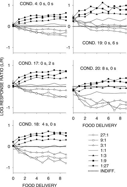
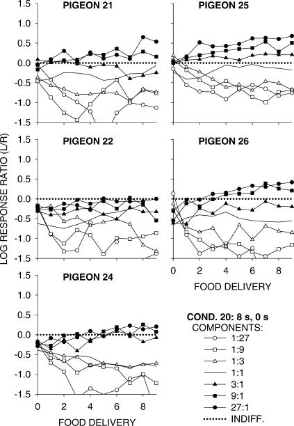
Figure 1 shows log response ratio (choice) in Phase 1 in each component (food–rate ratio) as a function of the number of food deliveries in the component. Appendix Figure A1 shows individual-pigeon results from Condition 20 to demonstrate that the group results fully represented those from the individuals. Log response ratio at zero on the x-axis, for example, shows choice before any food had been delivered in the component, and log response ratio at one food delivery was calculated for the period between the first and second food deliveries. Figure 1 also shows how choice changed across conditions as payoff delays were changed. As we have reported previously (e.g., Davison & Baum, 2000), choice in each component came to be controlled by the food ratio in that component as the number of food deliveries increased, and the degree of control tended to level off after four to six food deliveries. The degree of control across conditions (the vertical spread of the functions at the final three component food deliveries) changed in no systematic way, though the spread for Condition 4 (which came from the previous experiment) was smaller than the others. Variations in the delays typically moved all log response ratios toward the shorter delay, especially when the delay differences were greater. In fact, the choice trajectories became more and more asymmetrical around those for equal food rates (1∶1 ratio) as the longer delay increased to 8 s—response ratio changed more on the alternative that produced a shorter delay at a higher rate. Similar asymmetries were reported by Davison and Baum (2003) for differences in magnitude. Since the results shown in Figure 1 are representative of both previous research and of those obtained in Phases 2 and 3 of this experiment and are less informative, no such analyses will be shown subsequently.

Fig 1. Phase 1.

Log Left/Right response ratios in each of the seven components as a function of increasing numbers of component food deliveries. The data were grouped over the 5 pigeons. The dotted line represents indifference (equal choice). Appendix Figure A1 shows individual-pigeon results from Condition 20.

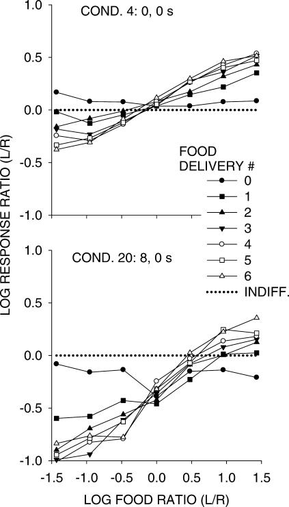
The vertical spread of choice in Figure 1 represents the degree to which choice was sensitive to differences in component food ratio after different numbers of component food deliveries. Figure 2 shows some of the log response ratios from Figure 1 plotted as a function of log food–rate ratio. The change in differential control across food-delivery number appears in steepening of the functions as more food deliveries occurred. In Condition 4 (equal 0-s delays), choice fell close to the origin (but with slight bias toward the left-key alternative); in Condition 20 (left delay 8 s, right delay 0 s), bias favored the right key, shifting all the functions downward. The results shown in Figure 2 were representative of the results in Phases 2 and 3 of this experiment.

Fig 2. Log Left/Right response ratios in Conditions 4 and 20 as a function of log food ratios for up to six component food deliveries.

The dotted line represents indifference (equal choice).

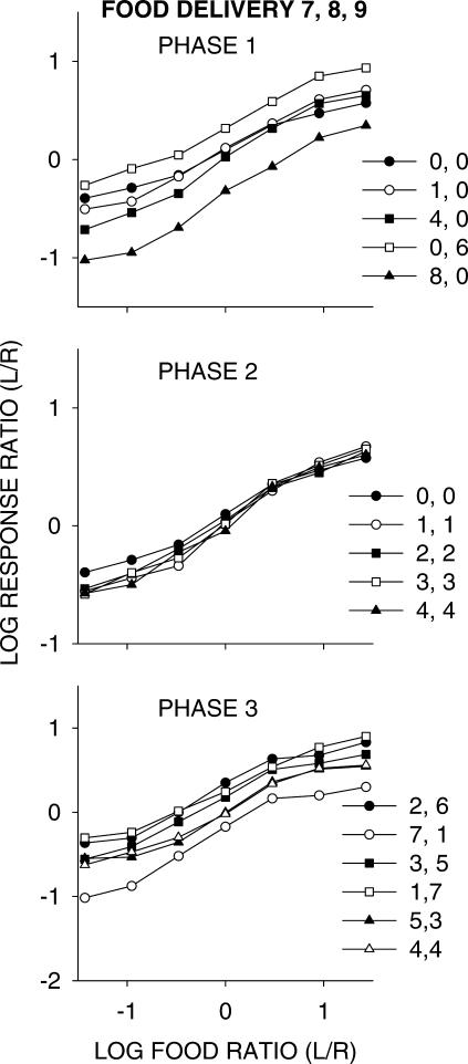
The analyses so far have shown that log response ratios were roughly asymptotic after four to six component food deliveries, as we have found previously (e.g., Davison & Baum, 2000). Thus, at this point we carried out a temporally extended analysis of choice in all three phases of the experiment before doing more local analyses. We used only the data obtained following component Food Deliveries 7, 8, and 9, for which the log response ratios were roughly asymptotic. Figure 3 shows choice from all phases of the experiment plotted as a function of the log food ratio across components within sessions with delay ratio (across sessions) as the parameter. Notable first is that the functions for all three phases deviated systematically from the straight lines that would be required by the generalized matching law (Baum, 1974). It might be thought that these deviations were caused by carryover from previous components (for example, a 27∶1 component will always be preceded by a component with a smaller food ratio). However, as we have shown frequently (Davison & Baum, 2000, 2003), carryover falls to zero after three to five component food deliveries. Thus, the shapes of the functions are caused by some other factor, and indeed may be described by the contingency-discriminability model proposed by Davison and Jenkins (1985; see also Davison & Nevin, 1999). This model is expressed in the equation:

2

where d_r measures the discriminability of the response–food contingencies, and c is bias. As d_r increases from 1.0 to infinity, the mixing of food deliveries decreases—that is, the confusion between alternatives vanishes. Table 2 shows optimal fits to the logarithmic transform of Equation 2 for each condition. The fits, as measured by variance accounted for, were excellent. The values of d_r were all similar and did not change systematically with delays or delay differences. The bias log c usually favored the smaller delay when the delays differed and was close to zero when the delays were equal. Figure 3 and the analyses in Table 2 suggest that the only effect of changing either relative or absolute delays on these relatively stable preferences was to change bias, a result unexpected from previous research on concurrent-chain schedules (e.g., Davison, 1983). The preferences were unlikely to have been completely stable, however, and longer components, even to 12 food deliveries, would probably have led to larger d_r (Baum & Davison, 2004; Davison & Baum, 2000).

Fig 3. Group choice as a function of relative food from the last three food deliveries in components.

Log Left/Right response ratio as a function of log food ratio (varied within sessions) for each pair of delays (varied between conditions) in all phases of the present experiment.

Table 2. Fits to the Davison and Jenkins (1985) model for concurrent-schedule performance. For each condition, responses following Food Deliveries 7, 8, and 9 in each component across all pigeons was combined and fitted by optimization to Equation 2 in logarithmic terms. Optimal values of response–food discriminability (d_r) and bias caused by the delays (log c) are shown with the proportion of data variance accounted for (VAC).

Condition	Phase	Delays (s)	dr	log c	VAC
4	1,2	0,0	3.41	0.08	1.00
17	1	0,2	5.00	0.10	1.00
18	1	4,0	5.59	−0.04	1.00
19	1	0,6	4.42	0.31	1.00
20	1	8,0	5.84	−0.39	0.99
21	2	1,1	4.73	0.02	0.99
22	2	2,2	4.08	0.05	1.00
23	2	3,3	4.50	0.05	1.00
24	2,3	4,4	4.25	0.02	0.99
25	3	2,6	4.73	0.27	0.99
26	3	7,1	5.58	−0.25	0.97
27	3	3,5	4.84	0.14	0.99
28	3	1,7	4.66	0.29	1.00
29	3	5,3	4.52	0.00	0.99
30	2,3	4,4	4.53	0	1.00

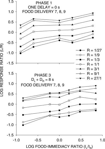
Figure 4 shows log response ratios after Food Deliveries 7, 8, and 9 plotted as a function of the right/left delay ratios in Phases 1 and 3 (omitting Phase 2, in which this ratio was 1.0). For the purpose of analysis, we set the zero delay to 1 s, probably longer than the time the pigeon took to access the food. Thus, the functions for Phase 1 are informative only of ordinal differences and trends. In Phase 3, however, the access delay would have been minimal (the pigeon would have been ready), so delay ratios are more exact. The lower plot in Figure 4 shows approximately linear and parallel changes in log response ratios with log delay ratios, with these functions being biased by log food–rate ratio. Again, such results were unexpected from concurrent-chains research (e.g., Duncan & Fantino, 1970; but see Berg & Grace, 2004), in which choice between pairs of delays depends only on the smaller of the two delays.

Fig 4. Phases 1 and 3.

Group choice as a function of relative delay from the last three food deliveries in components. Log Left/Right response ratio as a function of the Left/Right immediacy ratio (varied over conditions) according to the log food ratio (varied within sessions). Because the pigeons took an unknown time greater than 0 s to reach the food magazine, the preferences shown in the upper graph (Phase 1) have ordinal significance only, and the shapes of the functions are arbitrary. In Phase 3 (lower graph), the minimum delay was 1 s, presumably longer than the time pigeons took to move to the food magazine.

We analyzed each phase of the experiment in detail, using Equation 2 (expressed in logarithmic form) rather than Equation 1, because of the nonlinear relation between log response ratio and food ratio (Figure 3). However, when compared, the results of using Equation 2 were highly similar to the results of using Equation 1. Seven response ratios contributed to each fit of Equation 2, one from each of the seven components.

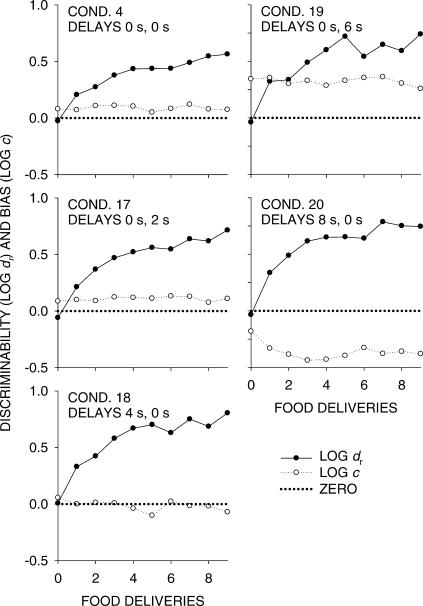
Figure 5 shows how discriminability and bias, measured in this way, changed with successive food deliveries in components in Phase 1, in which one delay was kept nominally at 0 s while the other was increased to 8 s. Discriminability (log d_r) increased as more food was delivered. Some tendency existed for log d_r to increase with greater difference between delays, consistent with the idea that the delay differential added to the discriminability of the alternatives based on the food differential. The inherent bias in Condition 4 favored the left key. The other biases shown constitute composites of this bias and bias due to the delay differential, which would favor the shorter delay. Bias usually grew stronger the larger the delay differential. Thus, Condition 19 shows a strong bias toward the left (0-s delay) over the right (6-s delay), and Condition 20 shows an even stronger bias toward the right (0-s delay) over the left (8-s delay). This result contradicts the steady-state finding that sensitivity to delay is low when one delay is very short (Duncan & Fantino, 1970)—that is, when one delay is 0 s, varying the other delay has little effect on preference. The present results suggest instead control by both delays.

Fig 5. Phase 1.

Response–food discriminability (d_r) and bias (log c) using Equation 2 for successive food deliveries in components. The dotted line represents zero discriminability and bias.

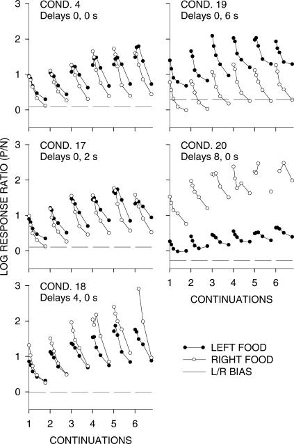
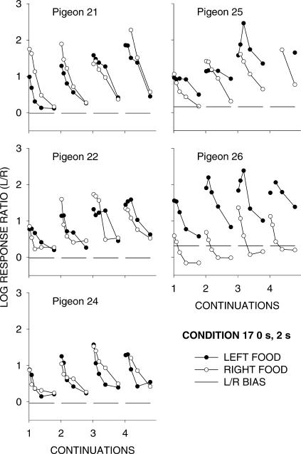
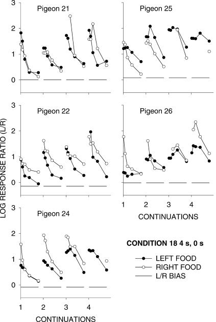
Figure 6 shows, for Phase 1, response ratios following food (in any component, at any location within components) as a function of the response number after food and according to increasing sequences of same-alternative food deliveries (continuations). The response numbers were grouped: all first responses, then second and third responses, then Responses 4 through 7, then Responses 8 through 15, and then Responses 16 through 31. The left/right response ratios for each curve were plotted against the x-axis at the centers of the bins: 0.5, 2.5, 5.5, 11.5, and 23.5. Figures A2 and A3 show the same analysis for individual pigeons for Conditions 17 and 18 (up to only four continuations because of decreasing response counts) to show that the group results were representative of individual-pigeon results. The effects resemble those found in previous experiments: Each food delivery was followed by a preference pulse to the just-productive alternative, and preference pulses became more extreme, and fell to progressively higher asymptotes, with increasing number of continuations. At delays of 6 and 8 s, pulse sizes after food decreased noticeably, whereas those after immediate food did not, even perhaps increasing as the delay at the other alternative increased.

Fig 6. Phase 1.

Group log response ratios to the just-productive alternative (P/N) following food on the left and right keys, and overall log Left/Right response ratios, in each condition. The response numbers were grouped: all first responses, then second and third responses, then Responses 4 through 7, then Responses 8 through 15, and then Responses 16 through 31. Each successive plot on a graph shows response ratios after 1, 2, 3, etc. successive food deliveries from the same alternative. The dashed line represents the overall Left/Right bias in each condition. Appendix Figure A2 shows individual-pigeon results from Condition 17 and 18.

To investigate this effect of delay at the other alternative, we conducted a detailed analysis of the heights of the pulses. We examined the change in absolute log response ratio across the five delays for each of the response bins after food. We fitted linear equations to log response ratio versus delay for each response bin, obtaining the slopes of the five lines. This was done for pulses after single food deliveries, for pulses after three continued food deliveries, and for pulses after five continued food deliveries. For pulses after the varied delay (0 to 8 s), these slopes were negative for all of the five response bins for pulses after any single food delivery, after three continuations, and also after five continuations. Thus, pulse heights did decrease with increasing delay. For the alternatives with 0-s delay, these slopes (log response ratio as a function of the alternative delay, 0 to 8 s) were positive for all five response bins for single food deliveries, and for three continuations. For continuations of five food deliveries, some of the log response ratios were infinite (exclusive to one alternative), so linear regressions could not be done for those particular responses. But the slopes were positive for all 29 response numbers on which regressions could be done. Thus, pulse heights on the constant alternative with 0-s delay increased as the delay on the other alternative increased, indicating that the effects of delay are not confined to the alternative with the longer delay, but are relative.

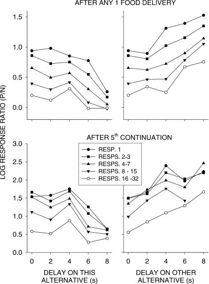
Figure 7 shows the results of a further analysis of the data presented in Figure 6, which investigated how the effect of delay changed during pulses. This figure shows log (P/N) response ratios from Figure 6 as a function of delay binned according to response number after food. The left-hand graphs show these data for the varied delay; the right graphs show these data after the constant delay. The upper graphs show the data after any single food delivery, and the lower graphs after five continued deliveries. We fitted straight lines between log response ratio and delay for the varied-delay alternatives (left graphs) for each response number after food (rather than for bins of response numbers shown in Figure 7). The slopes of these lines were negative, but appeared to become less negative for responses further from food. To investigate whether delay changes had similar effects at each response following food, straight lines were fitted to these slope estimates as a function of individual response number (1, 2, 3, etc.) for single food deliveries (slope  =  0.0011, standard error, SE  =  0.002), for three-food continuations (slope  =  0.002, SE  =  0.0001; not shown in Figure 7), and five-food continuations (slope  =  0.0023, SE  =  0.0002); that these slopes were positive revealed that the effect of delay decreased during the pulse. An identical analysis carried out for the 0-s alternative (right graphs) showed the positive slopes of the relations displayed in Figure 7 decreased toward zero across increasing response number after food for single food deliveries (slope  =  −0.0085, SE  =  0.0009), for three-food continuations (slope  =  −0.012, SE  =  0.003; not shown in Figure 7), and five-food continuations (slope  =  −0.048, SE  =  0.0048), indicating that the effect of the delay differential on the constant-delay pulse also decreased during the pulse. Thus, the response–ratio differential caused by differing delays decreased on both alternatives as responses increased in distance from prior food delivery. These results were again similar to those for amount of food (magnitude) differences (Davison & Baum, 2003), though we did not carry out such a detailed analysis.

Fig 7. Phase 1.

Group log response ratios to the just-productive alternative (P/N) as a function of delay (left graphs) and, for the 0-s delay alternative, as a function of delay on the other alternative (right graphs). Upper graphs show performance after any single food delivery, and lower graphs after five continued same-alternative food deliveries. Preferences are shown at selected response-number bins after food.

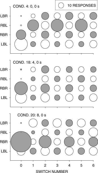
Figure 8 shows the results of an analysis at a more extended level, showing sequential visits to the two alternatives. In these bubble plots, the diameter of the circle shows the length (in pecks) of a visit. The x-axis represents visit number up to 6, the visits alternating left and right. The four rows of circles in each graph show sequences in which the first visit stayed at the just-productive alternative (left  =  LBL and right  =  RBR) and in which the first visit switched to the not-just-productive alternative (left  =  RBL and right  =  LBR). The results from three conditions are shown: 0 s, 0 s; 4 s, 0 s; and 8 s, 0 s. Three phenomena are apparent. First, the first visit following food was always the longest when responding stayed at the just-productive alternative, and when responding switched to the not-just-productive alternative (a relatively rare event) the visit was extremely short. These effects have been observed before in both rats (Aparicio & Baum, 2006) and pigeons (Baum & Davison, 2004). Second, when delays differed (Conditions 18 and 20), a stay visit following the short delay (0 s; RBR) exceeded a stay visit following the long delay (4 s or 8 s; LBL), the more so the longer the long delay. Moreover, relative to Condition 4 (0 s, 0 s), the lengths of both visits changed with increasing delay: The visit for the 0-s delay (filled circles) grew longer and the visit for the long delay (unfilled circles) grew shorter, indicating control by relative delay, rather than absolute delay. Third, when a clear disparity existed between initial stay visits at the two alternatives (as shown by the large difference between the circle sizes at switch Number 0 in Condition 20), it persisted up to the sixth visit. This persistent difference favoring the alternative with the shorter delay appears also in the sequences following a switched first visit. Such persistence of disparity in visits was observed before (Aparicio & Baum, 2006; Baum & Davison, 2004).

Fig 8. Phase 1, selected conditions.

Responses per visit as a function of switch number after food delivery for all pairwise sequences of food on the left and right keys. The length of the visit is shown by the diameter of the bubble. Unfilled bubbles are left-alternative visits, and filled bubbles are right-alternative visits, respectively.

A disparity between the alternatives' stay first visits (LBL and RBR) appears in Condition 4, in which the two alternatives had equal 0-s delays. Such a difference reflects a bias towards one key (the left). It also would presumably contribute to the bias parameter c in Equation 1 and Equation 2. It would presumably combine with preference generated by the delay differential, reducing the disparity between visits to the left and right when the longer delay was on the left (4 s, 0 s and 8 s, 0 s). We examine the effects of bias on visit length below.

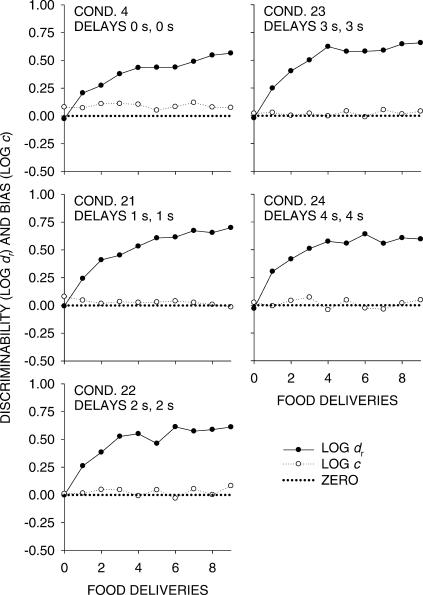
Figure 9, like Figure 5, shows changes in discriminability (log d_r in Equation 2) and composite bias (log c in Equation 2) as a function of successive component food deliveries, but in Phase 2 as both delays were increased together from 0 to 4 s. As in Phase 1, log d_r systematically increased across food deliveries, and the results resembled those for Phase 1 (Figure 5), except that log d_r remained about the same across delays from 1 to 4 s. Composite bias was close to zero and changed little as delay increased from 1 to 4 s.

Fig 9. Phase 2.

Response–food discriminability (d_r) and bias (log c) using Equation 2 for successive food deliveries in components. The dotted line represents zero discriminability and bias.

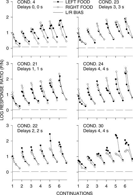
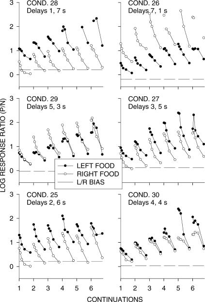
Similar to Figure 6, Figure 10 shows postfood preference pulses as a function of responses since food and as a function of continuations of food from one alternative. As would be expected, with equal delays there were no consistent differences in the height of pulses after left- and right-food deliveries, even within replicated Conditions 24 and 30. Indeed, the data from Condition 30 appeared to be more similar to those from Condition 4 than to Condition 24. Again, a detailed analysis as described above was carried out, this time averaging the absolute pulse heights across the two equal-delay (left and right) alternatives. Pulse heights did not change systematically across delay after single food deliveries (22/40 positive slopes for individual responses, rather than response bins as shown in Figure 10) or after three continuations (24/40 positive), but they did increase significantly with delay after five continuations (29/40 positive, z  =  2.69). Thus, as the delays were increased, no systematic change occurred in the size of postfood pulses, at least after a small number of continuations. An investigation of log response ratios versus delay across response numbers after food like that in Figure 7 showed that, for one, three, and five continued food deliveries, the slope of the choice–delay relation decreased systematically with response number. When the choice–delay slope was regressed against response number, the slopes of these relations for one, three, and five continued food deliveries were: −0.0006 (SE  =  0.0003); −0.0020 (SE  =  0.0003); and −.0023 (SE  =  0.0002). That these slopes were negative shows that the later the response after food the less the effect of delay on choice. That they became increasingly negative shows that the effects of delay were enhanced by longer runs of continuations.

Fig 10. Phase 2.

Group log response ratios to the just-productive alternative (P/N) following food on the left and right keys, and overall log Left/Right response ratios, in each condition. The response numbers were grouped: all first responses, then second and third responses, then Responses 4 through 7, then Responses 8 through 15, and then Responses 16 through 31. Each successive plot on a graph shows response ratios after 1, 2, 3, etc. successive food deliveries from the same alternative. The dashed line represents the overall Left/Right bias in each condition.

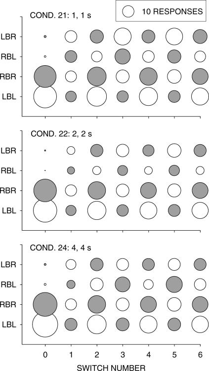
Figure 11 shows the results of an analysis of visits, similar to that shown in Figure 8, for Phase 2. The bubble plots are shown for three conditions: 1 s, 1 s; 2 s, 2 s; and 4 s, 4 s. The same sequential phenomena occurred: Stay first visits were longest, switched first visits were shortest, and subsequent visits (begun and ended by a switch) were intermediate. In contrast with Phase 1 (Figure 8), reflecting the equality of the delays, differences between visits to the two alternatives were small and unsystematic. In addition, no tendency was evident for the first visits to shorten as delays grew longer, contradicting what might be expected from the traditional idea of food strengthening the preceding response. Some hints of bias may be seen; these will be examined below.

Fig 11. Phase 2, selected conditions.

Responses per visit as a function of switch number after food delivery for all pairwise sequences of food on the left and right keys. The length of the visit is shown by the diameter of the bubble. Unfilled bubbles are left-alternative visits, and filled bubbles are right-alternative visits, respectively.

In Phase 3, the two delays summed to 8 s, and we varied the delays from 1 s and 7 s to 7 s and 1 s across conditions (Table 1). The data from Phase 3 lend themselves to a more comprehensive analysis than do those from Phases 1 and 2. We did this by expanding Equation 2 as follows:

3

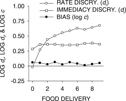
where I₁ and I₂ are the two immediacies and d_i is the discriminability between immediacies. Equation 3 was fitted to log response ratios calculated prior to each of the 10 food deliveries in components using multiple linear regression. Of the two independent variables, food–rate ratios were varied within conditions over seven levels, and food–immediacy ratios were varied across conditions over six levels, providing 42 response ratios for the fit for each food delivery. Figure 12 shows the results for the group data. The regressions fitted well, with variance accounted for of 71 and 90% for food deliveries 0 and 1, and between 95 and 97% following subsequent deliveries. Discriminability of food ratio (log d_r) increased from around 0 to around 0.65 over the 10 successive food deliveries as in Phases 1 and 2. Mean discriminability of immediacy ratio (log d_i) was 0.35, but the small increase was statistically significant (nonparametric trend test, z  =  2.15, p < .05, 2 tailed). This was due to the increase from Food Deliveries 0 to 1, however; across Food Deliveries 1 to 9 the trend was not significant. The mean bias (log c) was 0.04, indicating little overall key bias, and bias did not increase significantly with number of component food deliveries.

Fig 12. Phase 3.

Response–food discriminability (d_r), response–immediacy discriminability (d_i), and bias (log c) using Equation 3 for successive food deliveries in components (group data).

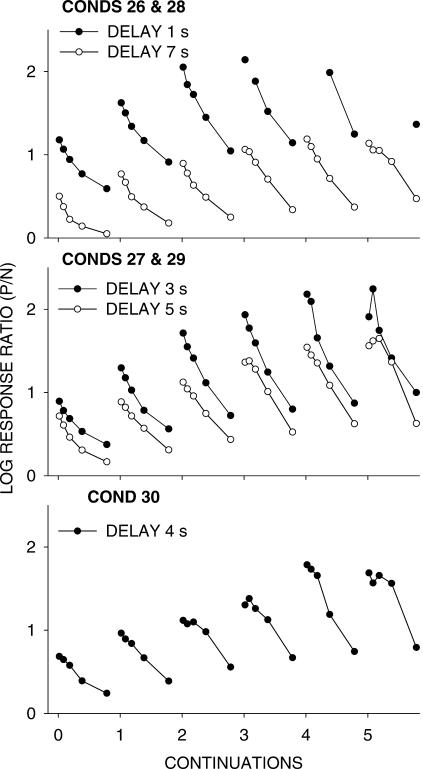
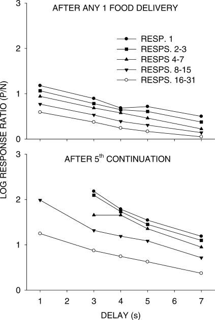
Similarly to Figures 6 (Phase 1) and 10 (Phase 2), Figure 13 shows preference pulses after single and continued food deliveries for Phase 3, and Figure 14 shows a condensed version of these results. In Figure 14, the absolute log response ratios for 4-s delay were averaged across the two alternatives; for the other graphs, the absolute pulses for particular delays were averaged across two conditions (e.g., the 1-s delay data were from the right-key alternative in Condition 26, and from the left-key alternative in Condition 28). Thus, the y-axis shows choice for the just-productive alternative (P) versus the not-just-productive alternative (N). Figure 14 shows that increasing delay (combined, here, with decreasing delay on the other alternative) decreased pulse height. A detailed analysis as described above showed that pulse height fell with increasing delay for each of the 40 successive individual responses (rather than response bins) for one, three, and five continuations (each p < .05, binomial test). Additionally, the effects of delay decreased with responses since food—that is, the negative slope across delays became less negative as responses were more distant from food. The choice–delay slope increased with response number for single food deliveries (slope  =  0.0012, SE  =  0.0001), for three continuations (slope  =  0.0028, SE  =  0.0001), and for five continuations (slope  =  0.0056, SE  =  0.0002). Figure 15 shows some of these effects. The y-axis represents log response ratio averaged across left and right, to give choice of the just-productive alternative (P) versus the not-just-productive alternative (N). Preference for alternative P was higher after 4 continuations (bottom graph) than after one food delivery (top graph) and decreased across delay for all response numbers. In addition, the dependence of preference on delay became flatter (less negative, hence increased toward zero) with increasing distance of the response from food.

Fig 13. Phase 3.

Group log response ratios to the just-productive alternative (P/N) following food on the left and right keys, and overall log Left/Right response ratios, in each condition. The response numbers were grouped: all first responses, then second and third responses, then Responses 4 through 7, then Responses 8 through 15, and then Responses 16 through 31. Each successive plot on a graph shows response ratios after 1, 2, 3, etc. successive food deliveries from the same alternative. The dashed line represents the overall Left/Right bias in each condition.

Fig 14. Phase 3.

Group log response ratios to the just-productive alternative (P/N) following food on the left and right keys, and overall log Left/Right response ratios, in each condition. The data have been averaged across the same delays arranged in different conditions; for instance, the 5-s delay data from Condition 29 (left key) were averaged with the 5-s delay data from Condition 27 (right key); the data for Condition 30 (equal 4-s delays) have been averaged across the left and right alternatives. Each successive plot on a graph shows response ratios after 1, 2, 3, etc. successive food deliveries from the same alternative.

Fig 15. Phase 3.

Log P/N response ratios as a function of delay duration at selected response number bins after food. The upper graph shows choice after any single food delivery, and the lower graph after five continued food deliveries on an alternative. The group data are the same as those used in Figure 14.

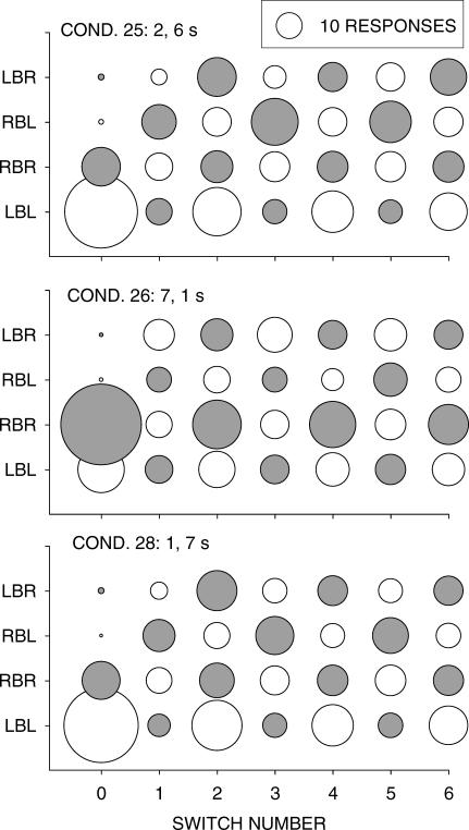
Figure 16 shows the results of an analysis of visits, similar to those shown in Figures 8 and 11, for Phase 3. Bubble plots are shown for three conditions: 2 s, 6 s; 7 s, 1 s; and 1 s, 7 s. Again, the large difference between stay first visits and switched first visits is evident, along with the intermediate length of subsequent visits begun and ended with a changeover. As in Figure 8, and in contrast with Figure 11, the first stay visits (LBL and RBR) following food varied with the duration of the delays. Comparing with Condition 24 (4 s, 4 s; Figure 11), we see that both visits changed; the visit following the shorter delay grew longer and the visit following the longer delay grew shorter. This again indicates control by relative delay and challenges a traditional view of food strengthening the preceding response.

Fig 16. Phase 3, selected conditions.

Responses per visit as a function of switch number after food delivery for all pairwise sequences of food on the left and right keys. The length of the visit is shown by the diameter of the bubble. Unfilled bubbles are left-alternative visits, and filled bubbles are right-alternative visits respectively.

Discussion

As food was more delayed, preference pulses following food delivery decreased. This effect was clearest in Phase 3 (Figures 13, 14, and 15), when the two delays summed to 8 s, but was also significantly present in Phase 1 (Figures 6 and 7). However, decreases in preference pulses with increasing delay were not found when both delays were equal (Phase 2), except following five continued food deliveries from an alternative, and then the effect was small. Thus, the size of preference pulses following food depended both on the duration of the delay on the chosen alternative and the duration of the delay on the other alternative—that is, on relative delay. This conclusion is supported by the results of Phase 1, in which preference pulses on the 0-s delay alternative increased when the delay on the other alternative was increased (Figures 6 and 7).

The analyses of visits also support the conclusion that performance was controlled by relative rather than absolute delay. Figure 8 shows that visits following the 0-s delay increased in length as the alternative longer delay increased. Figure 11 shows no effect as delay increased when the delays at the two alternatives were equal, discounting any effect of absolute delay. Figure 16 again shows control by relative delay, in that visits changed following both delays—increasing for the shorter delay and decreasing for the longer delay—in comparison with the baseline condition of equal 4-s delays (Figure 11).

The effects of the delay differential decreased with increasing numbers of responses since food, which means that the asymptotic level to which preference fell after food, although favoring the source of the latest food delivery, was not affected by delay differential. A comparable trend in visit length may be seen in Figures 8 and 16, where the differential between visits to the two alternatives decreased across successive visits. Thus, decreased delay and increased magnitude (Davison & Baum, 2003) and increased food rate (Baum & Davison, 2004; Davison & Baum, 2002) all have the same effect of increasing preference pulses and visit length following food. However, we cannot yet say whether rate and magnitude have relative effects as well as absolute effects because the relevant research has not been reported. Neither can we say, as yet, whether these choice-controlling variables have, in combination, additive effects on preference pulses, or whether the joint effects are less than additive. Further research in progress is designed to answer these questions.

In related research, Fantino and Royalty (1987) reported negative recency (i.e., negative preference pulses) in initial links after delayed food on concurrent-chains schedules. However, this effect (see also Killeen, 1970) occurred only when the initial-link concurrent VI VI schedules were independently arranged (that is, an alternative could continue to produce food even when a food delivery had been arranged on the other alternative). They reported no recency effect when interdependent (dependent) initial links were arranged. Since the present experiment used dependent scheduling, we have obtained a different result: positive recency using dependent schedules. The two experiments differ in a number of ways. First, data collection and the number of sessions of training were much greater in the present experiment. Second, Fantino and Royalty's arithmetic VI schedules arranged only 13 intervals and their exponential VI schedules only 20 intervals (presumably, the intervals were randomized from a list without replacement). With such limited numbers of intervals, the shortest interval, upon which recency would depend, tends to be relatively long. We used random-interval scheduling, which produces an exponential distribution of intervals, with a minimum interval of 1 s, and allocated food deliveries to alternatives probabilistically. Independent scheduling might have produced longer runs of food on the higher-rate alternative than would dependent scheduling—a consideration that would lead to positive recency in independent scheduling (Krägeloh et al., 2005)—opposite to the result reported by Fantino and Royalty. Our results, taken together with those of Krägeloh et al. suggest that the crucial factor producing positive recency (positive preference pulses), negative recency (negative preference pulses), or no recency is the relative likelihood of obtaining more food at the alternatives given that food has just been obtained from one of them. If the conditional probability is higher at the same alternative, then positive recency will occur; if the conditional probability is higher at the other alternative, then negative recency will occur.

The simplest explanation of the current positive-recency findings is that the relative value of the delayed food determined the subsequent preference pulse and visit length, because likelihood of right-key food following left-key food was unaffected by the left-key delay. Arguably, however, the value of food at the point at which it is delivered, whatever the delay, is the same. So, although the size of the preference pulse and length of the postfood visit are related to the delay, they must depend on the value of the food discounted by the delay in retrospect. Thus, potentially two processes contribute to initial-link preference in concurrent chains as they do in concurrent-schedule performance: One is an effect (positive recency here) produced by the food or terminal-link entry; the other may be the delay-discounted value of entering the terminal link (or, as some have suggested, the conditional reinforcing properties of the stimuli signaling the terminal links). The recency effect is, as Krägeloh et al. (2005) suggested, controlled by the conditional probability of further food signaled by a food delivery. The effect of discounted value is indicated by the level to which choice has fallen 16–31 responses after food (Figures 6, 10, and 13). To ask which of these is true preference would be futile; this research highlights the likely impossibility of comparing concurrent-schedule performances when the conditional probabilities of food signaled by food differ between experiments. Major differences in conditional probabilities will be caused by procedural variants such as independent versus dependent scheduling and the use of fixed lists of intervals (e.g., tapes) versus random-interval scheduling. The various ways of arranging concurrent VI VI initial-link schedules cause differences in the conditional probabilities of terminal-link entries and food between alternatives. If results cannot be compared across experiments using different procedures, fitting quantitative models across experiments will be fraught with error.

The size of a preference pulse depends on responding staying at the alternative that just produced food. If the first visit after food were randomly chosen, no pulse would occur. Control over the direction of the pulse must arise from the direction of the response before the delay (because a single food magazine was used), and we expect that such discriminative control would progressively decrease as delay lengthened. Hence, we might try to explain the smaller preference pulses with longer delays found in Phases 1 and 3 as a failure of discriminative control (i.e., forgetting). Harder to explain would be our findings that (a) preference pulse sizes (Figures 6 and 13) and visit lengths (Figures 8 and 16) were controlled by relative delay, and (b) preference pulses did not shrink nor did visit length decrease as equal delays were increased (Figures 10 and 11). Both of these findings are incompatible with the notion of decreasing discriminative control over pulse direction. Additionally, on the discriminative control hypothesis we would expect greater preference pulses when different delays are differentially signaled, as in Fantino and Royalty (1987), but they found no positive recency (i.e., no preference pulses) with dependent scheduling.

To summarize, our results suggest that pulse size, direction, and visit length are controlled only by the alternatives' prior relative value, with relative value determined by both delays, and with no decrement of discriminative control by delay. These processes would explain all three findings: (a) that pulse size and visit length depended on the delay prior to food; (b) that pulse size and visit length depended on the delay to food at the other alternative; and (c) that pulse size and visit length are unaffected when delays are equal.

A traditional molecular view would probably explain the first finding, dependence of preference pulse on delay, by referring to the gradient of delay of reinforcement. It would have difficulty, however, explaining the other two findings in a straightforward way. How would the effect of the delay at the other alternative be explained? How would the absence of an effect of delay when the delays are equal be explained? Perhaps explanations can be constructed, but we shall not try because we favor a molar view, which permits a straightforward explanation of these results.

What are the implications of these preference-pulse findings for models of choice averaged across the session in concurrent-chains schedules? Extended choice must be affected by the size and direction of preference pulses (Figures 6, 10, and 13). The present results indicate that the contribution of preference pulses depends on relative delay, a finding consonant with the contextual-choice model (CCM) of Grace (1994), in which the ratio of terminal-link delays is raised to a power that equals the ratio of the time spent in the terminal links over the time spent in the initial links. The longer the initial links, the smaller would be the contribution of postdelay pulses to extended preference or choice. Delay-reduction theory (Squires & Fantino, 1971) will do much the same. The hyperbolic-value added model (HVA; Mazur, 2001) would seem unable to deal with the relative-delay effects on preference pulses and hence their contribution to extended choice. But each of these models deals with the two clearly separable, and differently controlled, parts of initial-link preference (pulses and postpulse levels) as a single unit, whereas our results show they need to be dealt with separately in anything other than a purely descriptive model. These comments apply equally to existing models of concurrent-schedule performance.

Our research thus far indicates that longer relative delay and lower relative rate reduce the preference pulse and the visit length immediately after food delivery (Baum & Davison, 2004). Even though the food delivery is exactly the same for the two alternatives, if the food occurs at a lower relative rate, the preference pulse and visit length following food delivery are reduced. Similarly, even though the same food delivery occurs for both alternatives, the delay before the food affects preference after it. This leads us to conclude that the preference pulse is not due to the process traditionally called “reinforcement.” That is, if reinforcement means the immediate strengthening of the response that produced it, then our results must show that the very same “reinforcer” has different effects immediately following it, depending on temporally extended factors that precede it. Rather, we suggest that food delivery functions as a cue or discriminative stimulus signaling that further food is available for this activity (e.g., pecking at the left key), but subject to this delay and at this rate. The food guides behavior, rather than strengthening it in the traditional sense.

Appendix

Fig A1. Condition 20.

Log Left/Right response ratios in each of the seven components as a function of increasing numbers of component food deliveries for individual pigeons (cf. Figure 1). The dotted line represents indifference (equal choice).

Fig A2. Phase 1 Condition 17.

Individual-pigeon log response ratios to the just-productive alternative (P/N) following food on the left and right keys, and overall log Left/Right response ratios, in each condition (cf. Figure 6). Each successive plot on a graph shows response ratios after 1, 2, 3, etc. successive food deliveries from the same alternative. The dashed line represents the overall Left/Right bias in each condition.

Fig A3. Phase 1 Condition 18.

Individual-pigeon log response ratios to the just-productive alternative (P/N) following food on the left and right keys, and overall log Left/Right response ratios, in each condition (cf. Figure 6). Each successive plot on a graph shows response ratios after 1, 2, 3, etc. successive food deliveries from the same alternative. The dashed line represents the overall Left/Right bias in each condition.

References

- Alsop B, Elliffe D. Concurrent-schedule performance: Effects of relative and overall reinforcer rate. Journal of the Experimental Analysis of Behavior. 1988;49:21–36. doi: 10.1901/jeab.1988.49-21. [DOI] [PMC free article] [PubMed] [Google Scholar]
- Aparicio C.F, Baum W.M. Fix and sample with rats in the dynamics of choice. Journal of the Experimental Analysis of Behavior. 2006;86:43–63. doi: 10.1901/jeab.2006.57-05. [DOI] [PMC free article] [PubMed] [Google Scholar]
- Baum W.M. On two types of deviation from the matching law: Bias and undermatching. Journal of the Experimental Analysis of Behavior. 1974;22:231–242. doi: 10.1901/jeab.1974.22-231. [DOI] [PMC free article] [PubMed] [Google Scholar]
- Baum W.M, Davison M. Choice in a variable environment: Visit patterns in the dynamics of choice. Journal of Experimental Analysis of Behavior. 2004;81:85–127. doi: 10.1901/jeab.2004.81-85. [DOI] [PMC free article] [PubMed] [Google Scholar]
- Baum W.M, Rachlin H.C. Choice as time allocation. Journal of the Experimental Analysis of Behavior. 1969;12:861–874. doi: 10.1901/jeab.1969.12-861. [DOI] [PMC free article] [PubMed] [Google Scholar]
- Berg M.E, Grace R.C. Independence of terminal-link entry rate and immediacy in concurrent chains. Journal of the Experimental Analysis of Behavior. 2004;82:235–251. doi: 10.1901/jeab.2004.82-235. [DOI] [PMC free article] [PubMed] [Google Scholar]
- Chung S.H, Herrnstein R.J. Choice and delay of reinforcement. Journal of the Experimental Analysis of Behavior. 1967;10:67–74. doi: 10.1901/jeab.1967.10-67. [DOI] [PMC free article] [PubMed] [Google Scholar]
- Davison M. Bias and sensitivity to reinforcement in a concurrent-chain schedule. Journal of the Experimental Analysis of Behavior. 1983;40:15–34. doi: 10.1901/jeab.1983.40-15. [DOI] [PMC free article] [PubMed] [Google Scholar]
- Davison M, Baum W.M. Choice in a variable environment: Every reinforcer counts. Journal of the Experimental Analysis of Behavior. 2000;74:1–24. doi: 10.1901/jeab.2000.74-1. [DOI] [PMC free article] [PubMed] [Google Scholar]
- Davison M, Baum W.M. Choice in a variable environment: Effects of blackout duration and extinction between components. Journal of the Experimental Analysis of Behavior. 2002;77:65–89. doi: 10.1901/jeab.2002.77-65. [DOI] [PMC free article] [PubMed] [Google Scholar]
- Davison M, Baum W.M. Every reinforcer counts: Reinforcer magnitude and local preference. Journal of the Experimental Analysis of Behavior. 2003;80:95–129. doi: 10.1901/jeab.2003.80-95. [DOI] [PMC free article] [PubMed] [Google Scholar]
- Davison M, Baum W.M. Do conditional reinforcers count? Journal of the Experimental Analysis of Behavior. 2006;86:269–283. doi: 10.1901/jeab.2006.56-05. [DOI] [PMC free article] [PubMed] [Google Scholar]
- Davison M, Jenkins P.E. Stimulus discriminability, contingency discriminability, and schedule performance. Animal Learning and Behavior. 1985;13:77–84. [Google Scholar]
- Davison M, Nevin J.A. Stimuli, reinforcers, and behavior: An integration. Journal of the Experimental Analysis of Behavior. 1999;71:439–482. doi: 10.1901/jeab.1999.71-439. [DOI] [PMC free article] [PubMed] [Google Scholar]
- Duncan B, Fantino E. Choice for periodic schedules of reinforcement. Journal of the Experimental Analysis of Behavior. 1970;14:73–86. doi: 10.1901/jeab.1970.14-73. [DOI] [PMC free article] [PubMed] [Google Scholar]
- Elliffe D, Alsop B. Concurrent choice: Effects of overall reinforcer rate and the temporal distribution of reinforcers. Journal of the Experimental Analysis of Behavior. 1996;65:445–463. doi: 10.1901/jeab.1996.65-445. [DOI] [PMC free article] [PubMed] [Google Scholar]
- Fantino E, Royalty P. A molecular analysis of choice on concurrent-chains schedules. Journal of the Experimental Analysis of Behavior. 1987;48:145–159. doi: 10.1901/jeab.1987.48-145. [DOI] [PMC free article] [PubMed] [Google Scholar]
- Grace R.C. A contextual model of concurrent-chains choice. Journal of the Experimental Analysis of Behavior. 1994;61:113–129. doi: 10.1901/jeab.1994.61-113. [DOI] [PMC free article] [PubMed] [Google Scholar]
- Herrnstein R.J. Relative and absolute strength of response as a function of frequency of reinforcement. Journal of the Experimental Analysis of Behavior. 1961;4:267–272. doi: 10.1901/jeab.1961.4-267. [DOI] [PMC free article] [PubMed] [Google Scholar]
- Killeen P. Preference for fixed-interval schedules of reinforcement. Journal of the Experimental Analysis of Behavior. 1970;14:127–131. doi: 10.1901/jeab.1970.14-127. [DOI] [PMC free article] [PubMed] [Google Scholar]
- Killeen P. The matching law. Journal of the Experimental Analysis of Behavior. 1972;17:489–495. doi: 10.1901/jeab.1972.17-489. [DOI] [PMC free article] [PubMed] [Google Scholar]
- Kimble G.A. New York: Appleton-Century-Crofts; 1961. Hilgard and Marquis' Conditioning and learning (2nd ed.). [Google Scholar]
- Krägeloh C.U, Davison M, Elliffe D.M. Local preference in concurrent schedules: The effects of reinforcer sequences. Journal of the Experimental Analysis of Behavior. 2005;84:37–64. doi: 10.1901/jeab.2005.114-04. [DOI] [PMC free article] [PubMed] [Google Scholar]
- Landon J, Davison M, Elliffe D. Concurrent schedules: Short- and long-term effects of reinforcers. Journal of the Experimental Analysis of Behavior. 2002;77:257–271. doi: 10.1901/jeab.2002.77-257. [DOI] [PMC free article] [PubMed] [Google Scholar]
- Landon J, Davison M, Elliffe D. Concurrent schedules: Reinforcer magnitude effects. Journal of the Experimental Analysis of Behavior. 2003;79:351–365. doi: 10.1901/jeab.2003.79-351. [DOI] [PMC free article] [PubMed] [Google Scholar]
- Mazur J.E. Hyperbolic value addition and general models of animal choice. Psychological Review. 2001;108:96–112. doi: 10.1037/0033-295x.108.1.96. [DOI] [PubMed] [Google Scholar]
- McDevitt M.A, Williams B.A. Effects of signaled versus unsignaled delay of reinforcement on choice. Journal of the Experimental Analysis of Behavior. 2001;75:165–182. doi: 10.1901/jeab.2001.75-165. [DOI] [PMC free article] [PubMed] [Google Scholar]
- Omino T, Ito M. Choice and delay of reinforcement: Effects of terminal-link stimulus and response conditions. Journal of the Experimental Analysis of Behavior. 1993;59:361–371. doi: 10.1901/jeab.1993.59-361. [DOI] [PMC free article] [PubMed] [Google Scholar]
- Rachlin H. On the tautology of the matching law. Journal of the Experimental Analysis of Behavior. 1971;15:249–251. doi: 10.1901/jeab.1971.15-249. [DOI] [PMC free article] [PubMed] [Google Scholar]
- Squires N, Fantino E. A model for choice in simple concurrent and concurrent-chains schedules. Journal of the Experimental Analysis of Behavior. 1971;15:27–38. doi: 10.1901/jeab.1971.15-27. [DOI] [PMC free article] [PubMed] [Google Scholar]