

Abstract
We developed a new flexible approach for a co-analysis of multimodal brain imaging data using a non-parametric framework. In this approach, results from separate analyses on different modalities are combined using a combining function and assessed with a permutation test. This approach identifies several cross-modality relationships, such as concordance and dissociation, without explicitly modeling the correlation between modalities. We applied our approach to structural and perfusion MRI data from an Alzheimer’s disease (AD) study. Our approach identified areas of concordance, where both gray matter (GM) density and perfusion decreased together, and areas of dissociation, where GM density and perfusion did not decrease together. In conclusion, these results demonstrate the utility of this new non-parametric method to quantitatively assess the relationships between multiple modalities.
Keywords: Permutation, Combining function, Multiple modalities, Conjunction
Introduction
Often in neuroimaging studies, images from multiple imaging modalities are acquired from the same set of subjects. Even within MRI, for example, high-resolution structural images are often acquired together with low-resolution images of brain chemistry, blood flow, or function. Nevertheless, images produced by different modalities are often analyzed separately. To address this issue, different analysis methods, including multivariate (Chen et al., 2004; McIntosh et al., 1996) and univariate (i.e., voxel-by-voxel) (Pell et al., 2004; Richardson et al., 1997) approaches, have been suggested. In general, multivariate methods are preferable for exploring patterns and interregional networks in multi-modal data because they place few restrictions on patterns of associations (McIntosh and Lobaugh, 2004). For example, Chen et al. (2004) implemented a partial least square technique (McIntosh et al., 1996) for co-analyzing PET and structural MRI data. However, statistical inference based on multivariate methods often holds only in a global test for the entire brain and has limited ability to localize signals (Kherif et al., 2002; Worsley et al., 1997).
On the other hand, although model-based univariate methods make assumptions about associations, they are sometimes better suited for statistical inference. Several model-based univariate methods have been suggested for statistical inference of multiple modality images. In one approach (Richardson et al., 1997), images from different modalities were scaled to the same intensity range, and a linear regression model was fitted with different modalities modeled by indicator variables. Differences between modalities were assessed by contrasting these modality variables within the linear model (Richardson et al., 1997; Van Laere and Dierckx, 2001). Another approach in multi-modal co-analysis is the conjunction method, which identifies areas where significant changes overlap in multiple t statistic maps. This method, widely used in functional neuroimaging analyses (Friston et al., 1999; Nichols et al., 2005), was extended to multiple imaging modalities to identify conjunction (Pell et al., 2004).
A limitation of linear model and conjunction approaches is that these methods only identify one specific type of relationship between different modalities. The linear model approach only identifies areas where changes in one modality are larger than that of another, while the conjunction method only identifies the overlap of significant changes across modalities. Neither of these methods can be generalized to other types of relationships, including both positive and negative correlation.
Therefore, to overcome this shortcoming, we propose a general and flexible univariate non-parametric method, implementing co-analysis and identifying cross-modality relationships with combining functions and permutation testing (Hayasaka and Nichols, 2004). Furthermore, this method enables statistical inference without explicitly modeling the correlation across different imaging modalities (Hayasaka and Nichols, 2004; Lazar et al., 2002; Pesarin, 2001), since the cross-modality correlation is implicitly accounted for.
We evaluated the performance of this approach in a simulation-based validation. We also applied this approach to a multiple modality imaging data set of Alzheimer’s disease (AD) (Johnson et al., 2005) which is known to alter both brain structure as well as brain function (Karas et al., 2003; Matsuda et al., 2002; Minoshima et al., 1997). We investigated local changes in gray matter (GM) volume and cerebral perfusion, obtained by T1-weighted structural MRI and arterial spin labeling (ASL) perfusion MRI, respectively. Since changes in these two modalities do not necessarily occur in the same locations (Matsuda et al., 2002), we identified areas where structural and perfusion changes occur together (concordance) and areas where only one of these is observed but not the other (dissociation).
Methods
Combining functions
Our approach combines information from separate t images by a combining function, a function to combine multiple tests into a single test (Lazar et al., 2002; Pesarin, 2001), which is subsequently used in a statistical test. For example, for two modalities each with a t statistic image, S1 and S2, a combining function is defined, at an arbitrary voxel ν ∈ {(x, y, z)}, in a form
where S1(v), S2(v), and W(v) correspond to voxel values of t images S1 and S2, and the combining function image W, respectively. The function f is chosen so that a large value of W(v) corresponds to a relationship of interest between S1(v) and S2(v). For instance, let W(v) = S1(v) = S2(v), the product of two t values, which becomes large when both S1(v) and S2(v) increase or decrease together. When thresholded, W(v) defines a hyperbolic-shaped critical region in a 2D space of S1(v) and S2(v), sensitive to concordance between them, as seen in Fig. 1. By thresholding the combining function image W, areas where the relationship of interest occurs are identified. For interested readers, we present some suggestions of combining functions for different scenarios in Appendix A.
Fig. 1.

Examples of two-dimensional critical regions of W(v) = S1(v) = S2(v), with different threshold values.
Permutation test framework
Since the voxel value distribution of a combining function image is often unknown, we employ a permutation test for statistical inference (Holmes et al., 1996; Nichols and Holmes, 2002). Furthermore, when a combining function and a permutation test are used together, the correlation between t images is implicitly accounted for (Hayasaka and Nichols, 2004; Pesarin, 2001).
The permutation test works by generating the distribution of a test statistic based on random re-assignment, or permutation, of data labels. In our method, it operates in several steps. As an example, let us consider a two-group comparison setting on two imaging modalities, as illustrated in Fig. 2. First, group labels (A or B) are randomly reassigned to images of both modalities 1 and 2. Based on this random reassignment, two t statistic images, S1 and S2, are calculated on modalities 1 and 2, respectively. From these t images, a combining function image W is calculated. Although each voxel value W(v) can be considered as a test statistic, for multiple comparison correction, a summary statistic describing topological characteristics of W image needs to be selected. Such statistic – local maximum, cluster size, or some other statistics – is used in the subsequent test as a test statistic, rather than each voxel value W(v). Only the largest of such test statistics is recorded in each permutation, in order to control the family-wise error (FWE) rate to correct for multiple comparisons (Hayasaka and Nichols, 2003; Holmes et al., 1996). The entire process is repeated for a sufficient number of times, typically between 1000 and 3000 permutations for sufficient confidence in the permutation distribution, each with a different permutation of As and Bs. In the last permutation, the data labels are correctly assigned: As for A images and Bs for B images. Finally, an empirical distribution of the test statistic is generated by creating a histogram of all the recorded statistics. Corrected P values can be assessed by comparing the test statistic from the final permutation, the one with the correct group labels, to this empirical distribution.
Fig. 2.
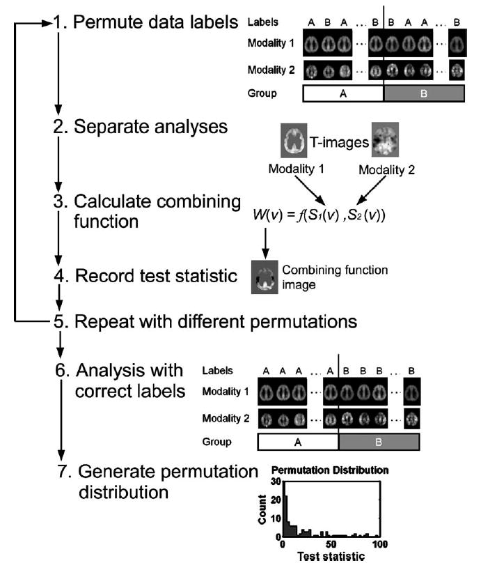
A schematic of the permutation test with a combining function. First, group labels (A/B) are randomly reassigned to images (1). Then based on this permutation of labels, t images are calculated separately (2). From the t images, a combining function is calculated (3), and the test statistic is recorded on the resulting combining function image (4). The entire process is repeated, each with a different permutation of labels (5). In the last permutation, data labels are correctly assigned (6). Finally, an empirical distribution of the test statistic is generated by creating a histogram of the test statistics (7). P values can be assessed by comparing the results from step (6) to the distribution found in step (7).
Simulation
To examine the performance of our method, we carried out a simulation-based validation. In each of 1000 realizations in this simulation, two sets of twenty 36 × 36 × 20 voxel images were generated. Each of the two sets was thought to be from one modality. To 10 images in each set, a sphere-shaped signal of radius r = 8 voxels was added. The locations of the signals were different in two modalities, with 3 different settings for the distance between the center of the signals: 0, r/2, and r (see Fig. 3). Larger distance means less overlap between the signals. Within each modality, a t image was calculated from a two-sample t test comparing images with and without the signal. The resulting t images from the two modalities, S1 and S2, with large t values at the locations of the respective signals, were combined by a combining function. The resulting combining function image was used as a statistic image in a permutation test with 100 permutations. In the permutation test, the cluster mass (Bullmore et al., 1999) was used as a test statistic, which is defined as the integration of the image intensity above the cluster defining threshold, calculated at each cluster. The cluster mass statistic is robust and sensitive to various signals, including localized high-intensity signals and spatially extended signals (Hayasaka and Nichols, 2004). The number of rejections at 0.05 significance level (FWE corrected) was recorded to calculate the power.
Fig. 3.

Locations of the signals in modalities 1 and 2. The distance between the centers of the signals were set to 0, r/2, and r, where r = 8 voxels is the radius of each signal.
We employed two combining functions in the simulation to assess the spatial relationship between signals in the two modalities. To assess the overlap of signals, we considered the concordance combining function Wc(v) defined as
| (1) |
This combining function is sensitive for large values of S1(v) and S2(v) occurring together. Critical regions of the concordance combining function are shown in Appendix A. We chose cluster defining thresholds to be 8 for Wc(v). To assess the signal occurring only in modality 1, we considered the dissociation combining function Wd(v), defined as
| (2) |
The width parameter λ, a positive number, controls the width of the critical region, whereas the shape parameter η, a positive integer, controls the shape of the critical region. A large (small) value of λ produces a narrow (wide) critical region, and a large (small) value of η widens (narrows) the base of the critical region, producing a rectangular (wedge) shaped critical region. The parameter η is multiplied by 2 to ensure concave critical regions. The critical regions corresponding to various values of λ and η are found in Appendix A. In this simulation, we used different values of λ (λ = 1/3, 1/2, and 2/3) and η (η = 1, 2, and 3). This combining function Wd (v) is sensitive to large values of S1(v) and near-zero values of S2(v) occurring together. The function Wd(v) can be seen as the value of S1(v) penalized by the term (λS2(v))2η, for S2(v) deviating from 0 (i.e., a change in modality 2). We chose the cluster-defining threshold to be 3 for Wd (v).
In a multiple-modality imaging study, it is possible that images in two different modalities have different smoothness despite smoothing. Thus, we considered a case where two imaging modalities having the same smoothness (FWHM = 6 and 6 voxels), and different smoothness (FWHM = 3 and 6 voxels for modalities 1 and 2, respectively).
Application
Our non-parametric method was applied to a co-analysis of GM volume changes in T1-weighted structural MRI and perfusion changes in ASL perfusion MRI. Twenty patients with a clinical diagnosis of probable AD according to the NINCDS-ADRDA (National Institute of Neurological and Communicative Disorders and Stroke–Alzheimer’s Disease and Related Disorder’s Association) criteria (McKhann et al., 1984) and 22 cognitively normal (CN) controls were included in this study. Their characteristics are summarized in Table 1.
Table 1.
Characteristics of subjects in the study
| Characteristics | Group
|
|
|---|---|---|
| AD | CN | |
| N (male/female) | 20 (13/7) | 22 (9/13) |
| Mean age (SD) | 72.9 (10.8) | 73.6 (7.6) |
| Mean MMSE score (range) | 21 (17–26) | 29.5 (28–30) |
Image acquisition and processing
All the subjects were scanned on a Siemens 1.5T Vision scanner (Erlangen, Germany). T1-weighted structural images were acquired using an MPRAGE (magnetization prepared rapid acquisition gradient-echo) sequence with TR/TE/TI = 10/7/300 ms, FA = 15°, and slice thickness = 1.4 mm. Perfusion weighted images (PWI) were acquired using the DIPLOMA (double inversions with proximal labeling of both tag and control images) pulsed ASL method (Jahng et al., 2003) with TR/TE = 2500/15 ms and post-inversion pulse time 1500 ms. For each perfusion scan, 5 slices of 8 mm thickness and 2 mm gap covering the volume above the AC-PC line were acquired with a single-shot gradient-echo EPI (echo-planar imaging) sequence. Details on the PWI acquisition can be found elsewhere (Johnson et al., 2005). Each PWI was co-registered to its corresponding T1-weighted image and corrected for partial volume effect (PVE) using a three-compartment model (Müller-Gärtner et al., 1992; Quarantelli et al., 2004).
T1-weighted and perfusion images were spatially normalized to a study-specific template. The study-specific template was created by averaging all the centered and aligned T1-weighted images. The T1-weighted images were also segmented (Ashburner and Friston, 1997; Ashburner and Friston, 2000), smoothed (6 mm isotropic Gaussian), and averaged to create tissue specific templates for GM, white matter (WM), and cerebrospinal fluid (CSF). Using these templates, T1-weighted images were normalized, segmented, and modulated according to the optimized voxel-based morphometry (VBM) protocol (Good et al., 2001) in SPM2 (Wellcome Department of Imaging Neuroscience; London, UK). Of the segmented images, only GM probability images were used in the subsequent analyses. The normalization parameters from the optimized VBM protocol (Ashburner and Friston, 1999; Good et al., 2001), both affine (12 parameters) and non-linear (10 × 9 × 10 discrete cosine basis functions), were applied to perfusion images to achieve normalization in the same template space. Normalized perfusion images were re-sliced to 2 × 2 × 2 mm voxel size for better use of spatial information and smoothed with a 12-mm Gaussian kernel to account for imperfection in co-registration and normalization. The GM images were similarly smoothed and re-sliced.
Statistical analysis
For each of the GM and perfusion data sets, a two-sample t test was performed separately to compare AD < CN. The GM t test was adjusted for age and total intra-cranial volume as covariates in an ANCOVA (analysis of covariance) model. In the resulting t image SGM, a large t value corresponded to GM loss in AD. The perfusion t test was adjusted for age and reference perfusion as covariates in an ANCOVA model. The mean perfusion value of the motor cortex was chosen as reference perfusion for each subject because this region is relatively spared from AD pathology (Braak et al., 1999). In the resulting t image Sperf, a large t value corresponded to reduced perfusion, or hypoperfusion, in AD.
In the permutation test, we applied the concordance combining function Wc(v) and the dissociation combining function Wd(v) to two t images from the GM and perfusion t tests. In particular, we defined
| (3) |
| (4) |
| (5) |
The combining function U(v) is sensitive to concordance between GM loss and hypoperfusion. On the other hand, V(v) and W(v) are sensitive to dissociation between GM and perfusion changes; while V(v) is sensitive to hypoperfusion without GM change, W(v) is sensitive to GM loss without perfusion change. Fig. 4 shows examples of critical regions defined by these combining functions in terms of SGM(v) and Sperf(v). In (4), we chose λ = 0.5 so that the critical region spans roughly from SGM(v) = − 2 to 2, and a typical t test fails to reject the null at P = 0.05 uncorrected significance level in such a critical region. Also in (4), we chose η = 2 for a wider critical region than a typical parabola at its base, enhancing sensitivity in that area. In (5), the width and shape parameters were similarly chosen as λ = 0.5 and η = 2. For interested readers, more discussions on parameters λ and η, as well as the shape of critical regions, can be found in Appendix A.
Fig. 4.
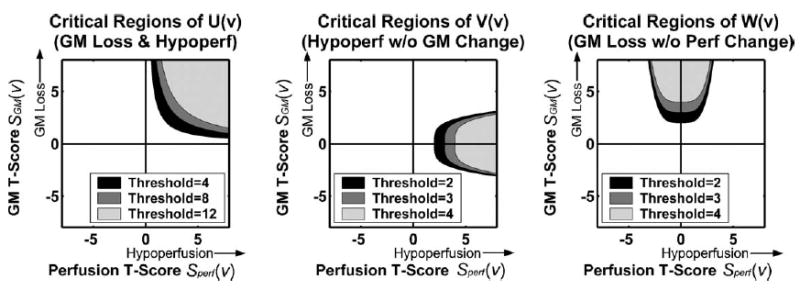
Examples of critical regions for concordance and dissociation combining functions.
Each of these combining function images was used as a statistic image in the permutation test. In the permutation test, the cluster mass was used as a test statistic. To implement the permutation test, we used a modified version of SnPM2b package (SnPM Authors, the University of Michigan; Ann Arbor, MI, USA), a non-parametric toolbox for SPM2. For each permutation test, 1000 permutations were carried out. Since the accuracy of P value estimates does not improve dramatically by running more permutations (e.g., standard error (SE) = 0.007 for 1000 permutations compared to SE = 0.004 for 3000 permutations, for a cluster with corrected P = 0.05 (Hayasaka and Nichols, 2003)), we limited the test to 1000 permutations in order to conserve time and disk space.
Sensitivity analysis
A sensitivity analysis was carried out in order to understand how much the analysis results are influenced by the choice of the width and shape parameters λ and η in the dissociation combining functions (4) and (5). In particular, a bootstrap analysis (Efron and Tibshirani, 1993) was performed in order to examine how the distribution of the largest cluster mass changes when λ and η are changed. In each of 100 bootstrap samples generated, combining functions (4) and (5) were calculated with different values of λ (λ = 1/4, 1/3, 1/2, 2/3, or 3/4) and η (η = 1, 2, 3, 4, 5), and the largest cluster mass was recorded for each combination of λ and η. The same cluster defining thresholds were used as in the actual analyses above.
Computing environment
The data analyses were performed on a Dell PC with a 3GHz Pentium 4 processor and 1GB of RAM, using MATLAB 6.5 (MathWorks; Natick, MA, USA). For each permutation test, computation time was under 20 min. The simulation and sensitivity analyses were performed on a Linux workstation using MATLAB 6.5.
Results
Simulation
Fig. 5 shows the plots of power for Wc(v) and Wd (v) for different signal settings, with two modalities having the same smoothness (a) and different smoothness (b).
Fig. 5.

The power of the permutation test with different combining functions for different signal settings in two modalities, under the same smoothness (a) or different smoothness in two modalities (b). The centers of signals are apart 0, r/2, and r, where r = 8 voxels is the radius of each signal (see Fig. 3). As the distance increases, the area of overlap between signals decreases.
The concordance combining function was sensitive when the overlap between the two signals was large. However, the power decreased as the distance increased and the area of overlap decreased. The concordance combining function seemed slightly more powerful when two modalities have different smoothness.
The dissociation combining function became more sensitive when the overlap between the signals became smaller. It appeared that, the larger the value of λ, more powerful the test became. In terms of η, the combining function was slightly more sensitive when η = 1 compared to η = 2 or 3. However, the difference in power between η = 2 and η = 3 was negligible. These findings were consistent in both smoothness settings (same or different smoothness), and the difference in power between these two settings was negligible.
These results indicate that the concordance and dissociation combining functions are calibrated to detect the relationship of interest between the two modalities.
Separate GM and perfusion analyses
The results from the separate GM and perfusion t tests are shown in Fig. 6a, in which areas of GM loss (green) and hypoperfusion (red) are shown. A liberal threshold was used in these results (P < 0.001 uncorrected) to give an overview of regional patters of GM loss and hypoperfusion. The pattern of GM loss was consistent with similar VBM studies of AD (Baron et al., 2001; Karas et al., 2003), with large areas of GM loss seen in the bilateral inferior and posterior parietal areas, as well as in the bilateral posterior cingulate cortices (PCC). The pattern of hypoperfusion was consistent with similar studies using PET and SPECT (Matsuda et al., 2002; Minoshima et al., 1997), with large areas of hypoperfusion in the right PCC and in the right posterior parietal area. Also a large area of hypoperfusion was seen in the right middle frontal gyrus with some extension into the superior frontal gyrus.
Fig. 6.
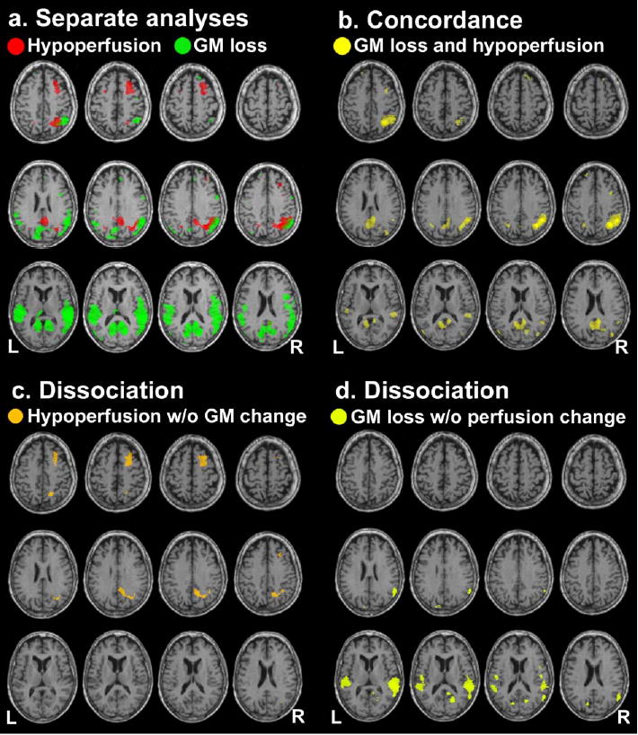
(a) Results from the separate analyses of GM and perfusion data. Areas of GM loss (green) and hypoperfusion (red) in AD compared to CN are indicated ( P < 0.001 uncorrected). (b) Results from the concordance analysis. Clusters of significant concordance (GM loss and hypoperfusion) are shown (U > 8 threshold, P < 0.05 corrected). (c) Results from the dissociation analysis (hypoperfusion without GM change). Clusters of significant dissociation are shown (V > 3 threshold, P < 0.05 corrected). (d) Results from the dissociation analysis (GM loss without perfusion change). Clusters of significant dissociation are shown (W > 4 threshold, P < 0.05 corrected).
Combining function thresholds
A scatter plot of all the voxel values of SGM and Sperf is shown in Fig. 7, with the cluster defining thresholds for the concordance and dissociation analyses overlaid. Each of these thresholds was chosen so that it was low enough for clusters to form, yet high enough for spatial localization of clusters.
Fig. 7.

A scatter plot of GM and perfusion t scores. The cluster defining thresholds for the concordance and dissociation analyses are also shown.
Concordance (GM loss and hypoperfusion)
Areas of concordance, GM loss and hypoperfusion occurring together, are shown in Fig. 6b (P < 0.05 corrected). Large clusters for concordance were mainly found in the bilateral PCC with some extension into the precunei, as well as in the right posterior parietal area. Some small clusters were also found in the left posterior parietal lobe and in the bilateral superior prefrontal areas. These concordance clusters identified the areas of overlap between GM loss and hypoperfusion seen in Fig. 6a.
Dissociation (hypoperfusion without GM change)
Areas of dissociation, hypoperfusion without GM change, are shown in Fig. 6c ( P < 0.05 corrected). A large dissociation cluster was found in the right PCC and precuneus, located superior to the concordance cluster found earlier. Another large dissociation cluster was found in the right middle frontal gyrus with some extension into the superior frontal gyrus.
Dissociation (GM loss without perfusion change)
Areas of dissociation, GM loss without perfusion change, are shown in Fig. 6d (P < 0.05 corrected). Large dissociation clusters were found in the bilateral inferior parietal areas, and a few small dissociation clusters were seen in the bilateral PCC and precunei inferior to the concordance cluster found earlier.
Sensitivity analysis
Fig. 8 shows plots of the median of the largest cluster mass from bootstrap samples, as well as the inter-quartile range, for various values of the width parameter λ (top) and the shape parameter η (bottom). These results are from the dissociation combining function for hypoperfusion without GM change (4), but the results are similar for the combining function for GM loss without perfusion change (5) (not shown). From the figure, it can be seen that a change in λ influenced the distribution of the largest cluster mass. A small value of λ produced larger clusters, possibly due to a wide critical region. On the other hand, a large value of λ produced smaller clusters, possibly due to a narrow critical region. The value of η seems to have only a slight influence on the analysis results.
Fig. 8.

The results from the sensitivity analysis by bootstrapping. The median of the bootstrap largest cluster mass from the dissociation combining function (hypoperfusion without GM change) is shown as a function of λ at η = 2 (top) and as a function of η at λ = 1/2 (bottom). Inter-quartile ranges are also shown.
Discussion
The proposed new method quantitatively assesses different relationships between GM and perfusion changes, using a simple and flexible non-parametric framework consisting of a combining function and a permutation test. In contrast to previous methods for analysis of multi-modality imaging, our approach is highly versatile; different cross-modality relationships are examined using the same permutation test framework just by selecting appropriate combining functions. Even though different combining functions were used in different analyses, no explicit modeling of voxel value distribution and cross-modality correlation was needed, as these were modeled implicitly in a combining function and a permutation test. Implicit modeling of the inter-modality correlation was particularly an important property in our analyses, since it is reasonable to assume that perfusion and GM volume are somewhat correlated (Ibáñez et al., 1998; Kanetaka et al., 2004; Matsuda et al., 2003).
In our concordance analysis, we found GM loss and hypo-perfusion (despite PVE correction) in the posterior parietal lobe and PCC. Thus, hypoperfusion in these areas is greater than that expected from GM loss (Ibáñez et al., 1998). From our dissociation analyses, we found hypoperfusion without GM change in the PCC (superior to the concordant region) and middle frontal gyrus. Such hypoperfusion may be due to deafferentation of these regions resulting from GM loss in other remotely connected brain regions (Braak et al., 1999; Meguro et al., 2001; Mielke et al., 1996). We also found GM loss without perfusion change in inferior parietal areas and in the PCC inferior to the concordant region. In these areas, perfusion loss may not be reduced beyond the level expected from GM loss. Overall, our findings were consistent with the results of a previous neuroimaging study using MRI and SPECT (Matsuda et al., 2002), in which areas of reduced GM volume and cerebral perfusion were observed in the posterior part of the brain, while hypoperfusion was more apparent than GM loss in frontal brain regions. Further studies are needed to investigate the clinical significance of these findings.
Our approach can be easily implemented in co-analyses of other MRI imaging modalities or even extended to other modalities such as PET or SPECT imaging. Furthermore, this method can be generally extended to more than two modalities. For instance, in addition to GM loss and hypoperfusion in our example, an investigator might be interested in functional decline associated with these structural as well as physiological changes. In such case, the investigator may examine concordance among three modalities, structural MRI, ASL perfusion MRI, and BOLD functional MRI, by using a combining function
where SfMRI corresponds to a t image associated with functional decline among AD patients. This combining function is sensitive for GM loss, hypoperfusion, and functional decline occurring together. Our method is also useful in longitudinal studies to capture changes of different modalities over time, which might provide deeper insight in disease progression.
In this approach, there are obstacles and limitations that should be mentioned. First, as in other multi-modality imaging methods, co-registering and normalizing different imaging modalities are not simple, since some imaging modalities are more prone to distortions and artifacts than other modalities. A limitation specific to our approach is that selection of combining functions is arbitrary and subjective. A combining function is chosen according to a user’s interest, and there is an infinite number of possible combining functions to choose from. For our dissociation combining functions V(v) and W(v), for example, there are many possibilities for the choice of parameters λ and η in (4) and (5). Furthermore, in addition to a polynomial form as seen in these functions, there are other possible forms of combining functions, such as trigonometric, logarithmic, or exponential functions, and combinations thereof. Clearly it is impossible to evaluate all possible combining functions objectively, but a combining function can be chosen from a handful of candidates. As it can be seen from our simulation and sensitivity analysis, we can evaluate sensitivity and robustness of combining functions from a simulation and a sensitivity analysis, respectively. Interested readers can also choose a combining function from the ones suggested in Appendix A according to their hypotheses. Another limitation specific to our approach is lack of weighting mechanism to correct for variability difference between modalities. For example, in our concordance combining function U(v), there is no weighting for SGM(v) or Sperf(v), even though SGM(v) seems to be less variable than Sperf(v) (see Fig. 7). A difference in degrees of freedoms could also result in variability difference between modalities. To correct this problem, some sort of weighting mechanism (Hayasaka and Nichols, 2004) could be employed, but determining optimal weights could raise another challenge.
In conclusion, we have developed a non-parametric method for co-analysis of multi-modal brain imaging data and demonstrated its effectiveness in structural and perfusion MRI data. This approach can be implemented in co-analyses of other MRI, PET, or SPECT imaging modalities, improving analyses and interpretation of findings in multi-modal imaging studies.
Acknowledgments
This work was supported in part by VA Research Service (MIRECC), VA REAP, and NIH grants (AG10897 and NS40321).
Appendix A. Examples of combining functions
To facilitate selection of appropriate combining functions, we present examples of combining functions for four possible scenarios. In a study with two modalities 1 and 2, let S1 and S2 be the t statistic images based on the contrast of interest, respectively. Then we consider situations where our interests are:
Changes or effects in the same direction in both modalities
Changes or effects in opposite directions
Changes or effects observed in one of the modalities, but not the other
Comparing the magnitude: of changes or effects between modalities
A.1. Changes in the same direction
To identify changes or effects in the same direction in both modalities 1 and 2, we need to define a combining function which becomes large when both S1 and S2 are highly positive or negative at the same time. In such cases, we should choose combining functions whose critical regions are in the top-right quadrant or in the bottom-left quadrant, as seen in Fig. 9a. If we are interested in both S1 and S2 being positive (negative), then the critical region should be in the top-right (bottom-left) quadrant. The concordance combining function
Fig. 9.
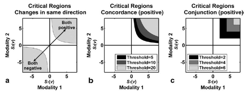
(a) To identify changes in the same direction, critical regions have to be in the top-right or bottom-left quadrant. (b) Critical regions of the positive concordance combining function with different thresholds. (c) Critical regions of the conjunction combining function with different thresholds.
| (6) |
is a possible combining function in this setting. Critical regions of this combining function can be limited to positive changes in the top-right quadrant by constraining S1(v) > 0 and S2(v) > 0 (Fig. 9b), or to negative changes in the bottom-left quadrant by constraining S1(v) < 0 and S2(v) < 0. Another possible combining function is the conjunction combining function
| (7) |
This is a non-parametric equivalent of the conjunction method mentioned in the Introduction (Nichols et al., 2005). This combining function identifies the overlap of areas S1(v) > w and S2(v) > w, for an arbitrary threshold value w (Fig. 9c).
A.2. Changes in opposite directions
To identify changes or effects in opposite directions in modalities 1 and 2, we need to define a combining function which becomes large when either S1 or S2 is highly positive, and the other is highly negative at the same time. In such cases, we should choose combining functions whose critical regions are in the top-left quadrant or in the bottom-right quadrant, as seen in Fig. 10. Critical regions on the bottom-right quadrant are sensitive to S1(v) being highly positive and S2(v) being highly negative occurring together, while critical regions on the top-left quadrant are sensitive to S1(v) being highly negative and S2(v) being highly positive occurring together. This can be achieved by negating either S1(v) or S2(v) in combining functions (6) and (7).
Fig. 10.
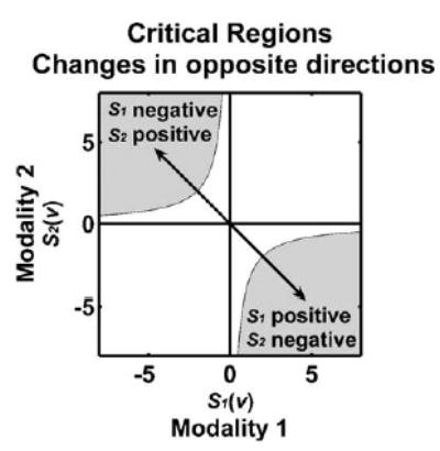
To identify changes in opposite directions, critical regions have to be in the bottom-right or top-left quadrant.
For example, by negating S1(v), the concordance combining functions (6) becomes
| (8) |
Similar to (6), critical regions for (8) can be limited to the bottom-right quadrant (S1(v) > 0 and S2(v) < 0) or top-left quadrant (S1(v) < 0 and S2(v) > 0), as seen in Figs. 11a and b, respectively. The critical regions for the conjunction combining function are in the bottom-right quadrant if S2(v) is negated (9), and in the top-left quadrant if S1(v) is negated (10),
Fig. 11.
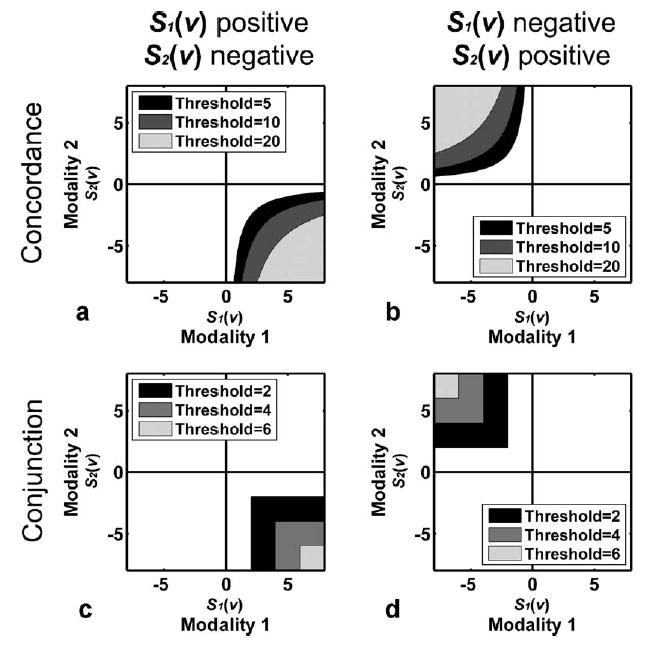
Critical regions for the concordance (top) and conjunction (bottom) combining functions with different thresholds, for positive S1(v) and negative S2(v) (left), as well as for negative S1(v) and positive S2(v) (right).
| (9) |
| (10) |
as seen in Figs. 11c and d, respectively.
A.3. Changes in one modality only
If we are interested in, for instance, changes occurring in modality 1 but not in modality 2, we need to choose a combining function whose critical regions are along the horizontal axis toward highly positive value of S1(v) (Fig. 12). Such combining function is sensitive to highly positive values of S1(v) (i.e., a large change in modality 1) and near-zero values of S2(v) (i.e., little change in modality 2). The dissociation combining function is suitable for such situation, which is defined as
Fig. 12.
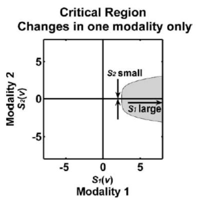
To identify changes in modality 1 but not in modality 2, critical regions need to be along the horizontal axis to identify large values of S1(v) and near-zero values of S2(v) occurring together.
| (11) |
where λ is the width parameter, and η is the shape parameter. The width parameter λ, a positive number, controls the width of the critical region; a large (small) value of λ produces a narrow (wide) critical region (Fig. 13a). The shape parameter η, a positive integer, controls the shape of the critical region; a large (small) value of η widens (narrows) the base of the critical region, producing a rectangular (wedge) shaped critical region (Fig. 13b). The parameter η is multiplied by 2 so that the critical region is concave. Though it is not feasible to perform an exhaustive search to determine the optimal values of λ and η, it is possible to decide these values among a list of possible values a priori by a simulation as demonstrated above.
Fig. 13.
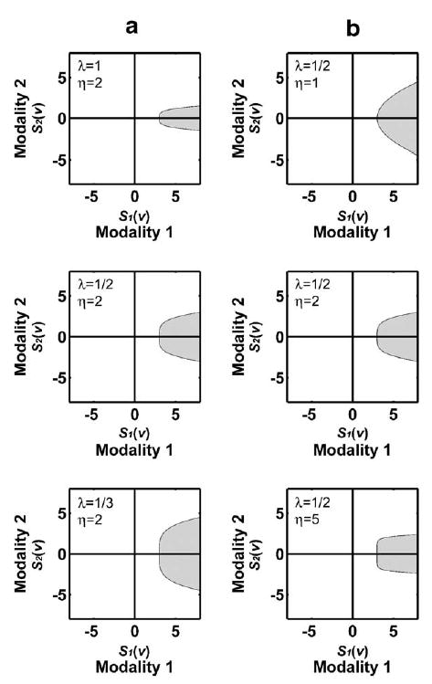
Critical regions of the dissociation function at threshold = 3, with different values of λ (a) and η (b). A large (small) value of λ produces a narrow (wide) critical region. A large (small) value of η widens (narrows) the base of the critical region, producing a rectangular (wedge) shaped critical region.
A.4. Comparing changes between modalities
If we are interested in comparing changes between two modalities, we can choose combining functions whose critical region is above or below the S1(v) = S2(v) line (Fig. 14), depending on the inequality (S1(v) < S2(v) or S1(v) > S2(v), respectively). For example, if we hypothesize that S1(v) is larger than S2(v) (i.e., changes in modality 1 is larger than that of modality 2), then we can define a combining function
Fig. 14.

In order to compare changes in two modalities, critical regions have to be above or below the S1(v) = S2(v) line, depending on the inequality. For example, if we hypothesize S1(v) > S2(v), then we can use a combining function X(v) = S1(v) − S2(v) whose critical regions lie below the S1(v) = S2(v) line.
| (12) |
This is a non-parametric equivalent of Richardson et al.’s (1997) method discussed in the Introduction. Fig. 14 shows examples of critical regions for this combining function.
This combining function is also useful in a longitudinal study setting. For example, if images are acquired on two different time points, then t images at the 1st and 2nd time points can be compared using (12). One advantage of such approach over a paired t test is that covariates, such as neuropsychological test scores, can vary across the two time points.
References
- Ashburner J, Friston K. Multimodal image coregistration and partitioning—A unified framework. NeuroImage. 1997;6 (3):209–217. doi: 10.1006/nimg.1997.0290. [DOI] [PubMed] [Google Scholar]
- Ashburner J, Friston KJ. Nonlinear spatial normalization using basis functions. Hum Brain Mapp. 1999;7 (4):254–266. doi: 10.1002/(SICI)1097-0193(1999)7:4<254::AID-HBM4>3.0.CO;2-G. [DOI] [PMC free article] [PubMed] [Google Scholar]
- Ashburner J, Friston KJ. Voxel-based morphometry—The methods. Neuroimage. 2000;11 (6 Pt 1):805–821. doi: 10.1006/nimg.2000.0582. [DOI] [PubMed] [Google Scholar]
- Baron JC, Chetelat G, Desgranges B, Perchey G, Landeau B, de la Sayette V, Eustache F. In vivo mapping of gray matter loss with voxel-based morphometry in mild Alzheimer’s disease. NeuroImage. 2001;14 (2):298–309. doi: 10.1006/nimg.2001.0848. [DOI] [PubMed] [Google Scholar]
- Braak E, Griffing K, Arai K, Bohl J, Bratzke H, Braak H. Neuropathology of Alzheimer’s disease: what is new since A. Alzheimer? Eur Arch Psychiatry Clin Neurosci. 1999;249 (Suppl 3):14–22. doi: 10.1007/pl00014168. [DOI] [PubMed] [Google Scholar]
- Bullmore ET, Suckling J, Overmeyer S, Rabe-Hesketh S, Taylor E, Brammer MJ. Global, voxel, and cluster tests, by theory and permutation, for a difference between two groups of structural MR images of the brain. IEEE Trans Med Imag. 1999;18 (1):32–42. doi: 10.1109/42.750253. [DOI] [PubMed] [Google Scholar]
- Chen K, Reiman EM, Caselli R, Bandy D, Alexander GE. Linking functional and structural brain networks: study of normal aging using the partial least square and dimension reduction techniques. Neurobiol Aging. 2004;25 (S2):269. [Google Scholar]
- Efron B, Tibshirani RJ. An Introduction to the Bootstrap. Chapman and Hall/CRC; Boca Raton, FL: 1993. [Google Scholar]
- Friston KJ, Holmes AP, Price CJ, Buchel C, Worsley KJ. Multisubject fMRI studies and conjunction analyses. NeuroImage. 1999;10 (4):385–396. doi: 10.1006/nimg.1999.0484. [DOI] [PubMed] [Google Scholar]
- Good CD, Johnsrude IS, Ashburner J, Henson RN, Friston KJ, Frackowiak RS. A voxel-based morphometric study of ageing in 465 normal adult human brains. NeuroImage. 2001;14 (1 Pt 1):21–36. doi: 10.1006/nimg.2001.0786. [DOI] [PubMed] [Google Scholar]
- Hayasaka S, Nichols TE. Validating cluster size inference: random field and permutation methods. NeuroImage. 2003;20 (4):2343–2356. doi: 10.1016/j.neuroimage.2003.08.003. [DOI] [PubMed] [Google Scholar]
- Hayasaka S, Nichols TE. Combining voxel intensity and cluster extent with permutation test framework. NeuroImage. 2004;23 (1):54–63. doi: 10.1016/j.neuroimage.2004.04.035. [DOI] [PubMed] [Google Scholar]
- Holmes AP, Blair RC, Watson JD, Ford I. Nonparametric analysis of statistic images from functional mapping experiments. J Cereb Blood Flow Metab. 1996;16 (1):7–22. doi: 10.1097/00004647-199601000-00002. [DOI] [PubMed] [Google Scholar]
- Ibáñez V, Pietrini P, Alexander GE, Furey ML, Teichberg D, Rajapakse JC, Rapoport SI, Schapiro MB, Horwitz B. Regional glucose metabolic abnormalities are not the result of atrophy in Alzheimer’s disease. Neurology. 1998;50 (6):1585–1593. doi: 10.1212/wnl.50.6.1585. [DOI] [PubMed] [Google Scholar]
- Jahng GH, Zhu XP, Matson GB, Weiner MW, Schuff N. Improved perfusion-weighted MRI by a novel double inversion with proximal labeling of both tagged and control acquisitions. Magn Reson Med. 2003;49 (2):307–314. doi: 10.1002/mrm.10339. [DOI] [PMC free article] [PubMed] [Google Scholar]
- Johnson NA, Jahng GH, Weiner MW, Miller BL, Chui HC, Jagust WJ, Gorno-Tempini ML, Schuff N. Pattern of cerebral hypoperfusion in Alzheimer disease and mild cognitive impairment measured with arterial spin-labeling MR imaging: initial experience. Radiology. 2005;234 (3):851–859. doi: 10.1148/radiol.2343040197. [DOI] [PMC free article] [PubMed] [Google Scholar]
- Kanetaka H, Matsuda H, Asada T, Ohnishi T, Yamashita F, Imabayashi E, Tanaka F, Nakano S, Takasaki M. Effects of partial volume correction on discrimination between very early Alzheimer’s dementia and controls using brain perfusion SPECT. Eur J Nucl Med Mol Imaging. 2004;31 (7):975–980. doi: 10.1007/s00259-004-1491-3. [DOI] [PubMed] [Google Scholar]
- Karas GB, Burton EJ, Rombouts SA, van Schijndel RA, O’Brien JT, Scheltens P, McKeith IG, Williams D, Ballard C, Barkhof F. A comprehensive study of gray matter loss in patients with Alzheimer’s disease using optimized voxel-based morphometry. Neuro-Image. 2003;18 (4):895–907. doi: 10.1016/s1053-8119(03)00041-7. [DOI] [PubMed] [Google Scholar]
- Kherif F, Poline JB, Flandin G, Benali H, Simon O, Dehaene S, Worsley KJ. Multivariate model specification for fMRI data. NeuroImage. 2002;16 (4):1068–1083. doi: 10.1006/nimg.2002.1094. [DOI] [PubMed] [Google Scholar]
- Lazar NA, Luna B, Sweeney JA, Eddy WF. Combining brains: a survey of methods for statistical pooling of information. NeuroImage. 2002;16 (2):538–550. doi: 10.1006/nimg.2002.1107. [DOI] [PubMed] [Google Scholar]
- Matsuda H, Kitayama N, Ohnishi T, Asada T, Nakano S, Sakamoto S, Imabayashi E, Katoh A. Longitudinal evaluation of both morphologic and functional changes in the same individuals with Alzheimer’s disease. J Nucl Med. 2002;43 (3):304–311. [PubMed] [Google Scholar]
- Matsuda H, Ohnishi T, Asada T, Li ZJ, Kanetaka H, Imabayashi E, Tanaka F, Nakano S. Correction for partial-volume effects on brain perfusion SPECT in healthy men. J Nucl Med. 2003;44 (8):1243–1252. [PubMed] [Google Scholar]
- McIntosh AR, Lobaugh NJ. Partial least squares analysis of neuroimaging data: applications and advances. NeuroImage. 2004;23 (Suppl 1):S250–S263. doi: 10.1016/j.neuroimage.2004.07.020. [DOI] [PubMed] [Google Scholar]
- McIntosh AR, Bookstein FL, Haxby JV, Grady CL. Spatial pattern analysis of functional brain images using partial least squares. NeuroImage. 1996;3 (3 Pt 1):143–157. doi: 10.1006/nimg.1996.0016. [DOI] [PubMed] [Google Scholar]
- McKhann G, Drachman D, Folstein M, Katzman R, Price D, Stadlan EM. Clinical diagnosis of Alzheimer’s disease: report of the NINCDS-ADRDA Work Group under the auspices of Department of Health and Human Services Task Force on Alzheimer’s Disease. Neurology. 1984;34 (7):939–944. doi: 10.1212/wnl.34.7.939. [DOI] [PubMed] [Google Scholar]
- Meguro K, LeMestric C, Landeau B, Desgranges B, Eustache F, Baron JC. Relations between hypometabolism in the posterior association neocortex and hippocampal atrophy in Alzheimer’s disease: a PET/MRI correlative study. J Neurol, Neurosurg Psychiatry. 2001;71 (3):315–321. doi: 10.1136/jnnp.71.3.315. [DOI] [PMC free article] [PubMed] [Google Scholar]
- Mielke R, Schroder R, Fink GR, Kessler J, Herholz K, Heiss WD. Regional cerebral glucose metabolism and postmortem pathology in Alzheimer’s disease. Acta Neuropathol (Berl) 1996;91 (2):174–179. doi: 10.1007/s004010050410. [DOI] [PubMed] [Google Scholar]
- Minoshima S, Giordani B, Berent S, Frey KA, Foster NL, Kuhl DE. Metabolic reduction in the posterior cingulate cortex in very early Alzheimer’s disease. Ann Neurol. 1997;42 (1):85–94. doi: 10.1002/ana.410420114. [DOI] [PubMed] [Google Scholar]
- Müller-Gärtner HW, Links JM, Prince JL, Bryan RN, McVeigh E, Leal JP, Davatzikos C, Frost JJ. Measurement of radiotracer concentration in brain gray matter using positron emission tomography: MRI-based correction for partial volume effects. J Cereb Blood Flow Metab. 1992;12 (4):571–583. doi: 10.1038/jcbfm.1992.81. [DOI] [PubMed] [Google Scholar]
- Nichols TE, Holmes AP. Nonparametric permutation tests for functional neuroimaging: a primer with examples. Hum Brain Mapp. 2002;15 (1):1–25. doi: 10.1002/hbm.1058. [DOI] [PMC free article] [PubMed] [Google Scholar]
- Nichols T, Brett M, Andersson J, Wager T, Poline JB. Valid conjunction inference with the minimum statistic. NeuroImage. 2005;25 (3):653–660. doi: 10.1016/j.neuroimage.2004.12.005. [DOI] [PubMed] [Google Scholar]
- Pell GS, Briellmann RS, Waites AB, Abbott DF, Chan PCH, Jackson GD. Combined voxel-based analysis of volume and t2-relaxometry in temporal lobe epilepsy; International Society for Magnetic Resonance in Medicine 12th Scientific Meeting; Kyoto, Japan. 2004. p. 1299. [Google Scholar]
- Pesarin F. Multivariate Permutation Tests. Wiley; New York: 2001. [Google Scholar]
- Quarantelli M, Berkouk K, Prinster A, Landeau B, Svarer C, Balkay L, Alfano B, Brunetti A, Baron JC, Salvatore M. Integrated software for the analysis of brain PET/SPECT studies with partial-volume-effect correction. J Nucl Med. 2004;45 (2):192–201. [PubMed] [Google Scholar]
- Richardson MP, Friston KJ, Sisodiya SM, Koepp MJ, Ashburner J, Free SL, Brooks DJ, Duncan JS. Cortical grey matter and benzodiazepine receptors in malformations of cortical development. A voxel-based comparison of structural and functional imaging data. Brain. 1997;120 (Pt 11):1961–1973. doi: 10.1093/brain/120.11.1961. [DOI] [PubMed] [Google Scholar]
- Van Laere KJ, Dierckx RA. Brain perfusion SPECT: age- and sex-related effects correlated with voxel-based morphometric findings in healthy adults. Radiology. 2001;221 (3):810–817. doi: 10.1148/radiol.2213010295. [DOI] [PubMed] [Google Scholar]
- Worsley KJ, Poline JB, Friston KJ, Evans AC. Characterizing the response of PET and fMRI data using multivariate linear models. NeuroImage. 1997;6 (4):305–319. doi: 10.1006/nimg.1997.0294. [DOI] [PubMed] [Google Scholar]