Mapping an intrinsic MR property of gray matter in auditory cortex of living humans: A possible marker for primary cortex and hemispheric differences

Abstract

Recently, magnetic resonance properties of cerebral gray matter have been spatially mapped – in vivo – over the cortical surface. In one of the first neuroscientific applications of this approach, this study explores what can be learned about auditory cortex in living humans by mapping longitudinal relaxation rate (R1), a property related to myelin content. Gray matter R1 (and thickness) showed repeatable trends, including the following:

1. Regions of high R1 were always found overlapping posteromedial Heschl’s gyrus. They also sometimes occurred in planum temporale and never in other parts of the superior temporal lobe. We hypothesize that the high R1 overlapping Heschl’s gyrus (which likely indicates dense gray matter myelination) reflects auditory koniocortex (i.e., primary cortex), a heavily myelinated area that shows comparable overlap with the gyrus. High R1 overlapping Heschl’s gyrus was identified in every instance suggesting that R1 may ultimately provide a marker for koniocortex in individuals. Such a marker would be significant for auditory neuroimaging, which has no standard means (anatomic or physiologic) for localizing cortical areas in individual subjects.

2. Inter-hemispheric comparisons revealed greater R1 on the left on Heschl’s gyrus, planum temporale, superior temporal gyrus and superior temporal sulcus. This asymmetry suggests greater gray matter myelination in left auditory cortex, which may be a substrate for the left hemisphere’s specialized processing of speech, language, and rapid acoustic changes.

These results indicate that in vivo R1 mapping can provide new insights into the structure of human cortical gray matter and its relation to function.

Introduction

Spatially mapping gray matter structure over the cortical surface of living humans has led to new insights into numerous central nervous system processes, including learning, cognitive aspects of aging, and the progression of neurologic or psychiatric disease (Rosas et al., 2002; Sailer et al., 2003; Sowell et al., 2003; Draganski et al., 2004; Salat et al., 2004; Thompson et al., 2004; Narr et al., 2005). Most work along these lines has involved mapping gray matter thickness (Fischl and Dale, 2000; MacDonald et al., 2000). However, another potentially illuminating but almost completely unapplied approach involves mapping the intrinsic magnetic resonance (MR) properties of gray matter tissue (e.g., the longitudinal and transverse relaxation rates; Fischl et al., 2004). These properties are sensitive to various aspects of the cellular architecture of the gray matter (e.g., myelin and iron content), including aspects that change during development, with disease, or spatially between cortical architectonic areas (Besson et al., 1989; Vymazal et al., 1999; Steen et al., 2000; Yoshiura et al., 2000; Gelman et al., 2001). One possibility is that mappings of intrinsic MR properties may lead to new understanding of the neuronal differences between cortical regions. Another possibility is that they may provide a way to resolve – in individual, living subjects – cortical areas (e.g., Brodmann areas) usually only defined in classical histology. If the latter possibility were borne out, it would mean that functional neuroimaging data could be precisely related to cortical architectonic areas identified in the same subjects. This would obviate the need for the usual approximate methods for co-registering function and cortical areas (i.e., mapping functionally imaged brains into normalized coordinates, into surface-based coordinates or onto probabilistic atlases; Talairach and Tournoux, 1988; Fischl et al., 1999; Rademacher et al., 2001). The present study begins to examine what might be learned by mapping intrinsic properties of the gray matter in normal, living humans. Our investigations focus on the superior temporal lobe, the region of the cerebrum housing auditory cortex.

Our experiments mapped a particular intrinsic MR tissue property, R1 (i.e., the reciprocal of T1). R1, the longitudinal relaxation rate for protons excited in the imaging process, can depend on various microscopic tissue properties (e.g., see Gore and Kennan, 1999). However, a predominant factor influencing R1 is tissue myelin content (see Discussion), a point illustrated by the striking contrast between gray and white matter in R1-weighted (i.e., T1-weighted) images. Our approach involved estimating R1 for each voxel in the brain, segmenting the gray matter, and averaging R1 across the depth of the gray matter at finely spaced points covering the cortical surface (Fischl et al., 2004). The resulting mappings do not show detailed variations in R1 across the gray matter laminae, but rather show the spatial distribution in overall R1 over a 2D ‘‘sheet’’ covering the superior temporal lobe. In addition to mapping R1, we also mapped gray matter thickness, a basic morphological parameter that was obtained automatically in the process of segmenting the gray matter.

The specific goals of this study were three-fold. First, since R1 of auditory cortex has never been mapped before, and there are few data concerning its thickness, an initial objective was to establish the basic spatial patterns of R1 and thickness. Our examinations covered the superior temporal plane, including Heschl’s gyri, planum temporale (PT) and planum polare (PP). They also extended onto the superior temporal gyrus (STG) and into the superior temporal sulcus (STS). Both studied variables, R1 and thickness, showed repeatable spatial patterns across subjects.

The second objective of this study was to determine whether spatial mappings of R1 or thickness might be useful in distinguishing architectonic divisions of auditory cortex. At one level, we took an empirical approach, examining whether thresholded maps of either R1 or thickness revealed discrete regions that might be assignable to particular cortical areas. At another level, however, we were motivated by the hypothesis that auditory cortical areas might be resolvable as regional differences in R1 because of the overall myelination differences seen between cortical areas in previous histological work. In both humans and non-human primates, the auditory cortical areas of the superior temporal lobe form several major distinctions: a core area with histological features of primary sensory cortex (i.e., koniocortex or Brodmann area 41), belt areas flanking the core medially and laterally, and lateral parabelt areas (e.g., Kaas et al., 1999). These areas (and subareas thereof) have been distinguished based on a variety of anatomic criteria: cytoarchitectonic, myeloarchitectonic, immunohistochemical, and connectional (Brodmann, 1909; von Economo, 1929; Sarkisov, 1966; Hopf, 1968; Galaburda and Sanides, 1980; Rivier and Clarke, 1997; Hackett et al., 2001; Wallace et al., 2002). However, a distinction of particular relevance to the present study is in overall myelin content. The gray matter of the auditory core is characterized by high myelin content (reflecting a high density of thalamocortical connections) relative to immediately adjacent regions of the medial and lateral belt. The medial belt is considerably less myelinated than koniocortex throughout its extent. The lateral belt, while more myelinated than its medial counterpart, still appears generally less myelinated than the core. Because of the strong relationship between R1 and tissue myelin content, we reasoned that spatial mappings of R1 might show local regions of high R1 reflecting heavy myelination, including high R1 corresponding to koniocortex. Such regions were indeed found. They were most consistently seen overlapping posteromedial Heschl’s gyrus, the region of the superior temporal lobe containing auditory koniocortex.

While histological studies have shown that human auditory koniocortex overlaps posteromedial Heschl’s gyrus (the anterior one when there are two), they also show considerable inter-subject variability in the disposition and extent of koniocortex relative to the gyrus (Rademacher et al., 1993, 2001; Sweet et al., 2005). Therefore, the analyses of the present study were conducted on individual subjects and hemispheres so any variability could be appreciated. Importantly, high R1 overlapping posteromedial Heschl’s gyrus was identified in every instance, indicating that high R1 can potentially be used to mark koniocortex in individuals. Such a marker would be highly significant for studies attempting to relate auditory cortical function to structure because there is currently no routine means (anatomic or physiologic) for localizing koniocortex in vivo on an individual basis. In contrast to the retinotopic mappings used to isolate fields within visual cortex (Sereno et al., 1995), tonotopic mappings in auditory cortex are not easily obtained (Formisano et al., 2003). The ability to identify auditory koniocortex in individual subjects might prove to be especially important in the cases of auditory pathology where individual morphology can be grossly abnormal (e.g., dyslexia; Leonard et al., 1993) making localization of koniocortex by standard methods particularly susceptible to errors.

Our third objective was to examine auditory cortical gray matter for hemispheric differences. This objective was motivated at a general level by the many well-known functional and anatomical asymmetries of the temporal lobe (e.g., Efron, 1963; Geschwind and Levitsky, 1968; Zatorre et al., 2002). Here, we show that the R1 of gray matter is systematically greater on the left, especially in posterior parts of the superior temporal plane, on the STG, and in the STS. This asymmetry in R1 suggests more extensive neuronal myelination within the gray matter of left auditory cortex, which may be an anatomical substrate for the left hemisphere’s specialized role in processing speech, language and rapid acoustic changes.

Methods

Five subjects (24 to 39 years, mean = 30 years; 3 male; all right-handed) each participated in one imaging session. Subjects had no known neurological disorders and no tinnitus. Hearing thresholds of all subjects were normal (<20 dB HL) at all standard audiological frequencies from 250 to 8000 Hz.

This study was approved by the institutional committees on the use of human subjects at the Massachusetts Institute of Technology, Massachusetts Eye and Ear Infirmary, and Massachusetts General Hospital. All subjects gave their written informed consent.

Imaging

Subjects were imaged using a 1.5-T whole-body Siemens Sonata scanner a receive-only head coil, and a body coil for transmit. In each imaging session, four scans of the whole head (1 slab; 128 sagittal slices; 8 min) were acquired using a standard excitation-recovery pulse sequence (3D FLASH, TR = 20 ms, TE = 7.72 ms, resolution: 1.3 × 1.0 × 1.3 mm). Each scan used a different flip angle (α = 3, 5, 20 and 30° for subjects 1–4; 5, 10, 20 and 40° for subject 5). The four resulting data sets allowed an estimation of R1 (for each voxel in the brain) using the following relationship between image signal (S), pulse parameters (TR, α), and R1 (Nishimura, 1996):

$$S(TR,\alpha ,R1)=K\hspace{0.17em}sin\alpha \frac{1-e^{-T{R}^{\ast }R1}}{1-cos\alpha e^{-T{R}^{\ast }R1}}$$

K is a constant that depends on proton density, R2* and the receive bias field. R1 estimation and motion-correction were performed iteratively. Four subjects also had whole head scans using a standard MPRAGE sequence (TR = 2530 ms, TE = 3.3 ms, resolution: 1.3 × 1.0 × 1.3 mm).

Estimating gray matter R1 and thickness

R1 and thickness were estimated using models for the CSF/gray matter and gray/white matter surfaces (Fig. 1). Since the contrast between gray and white matter was not optimal in any individual FLASH scan (with a given flip angle), the surfaces were generated using a synthesized T1-weighted volume derived from the multiple FLASH data sets so as to achieve high contrast between gray and white matter (effective imaging parameters: TR = 20 ms; α= 30°; TE = 3 ms). The surface models were generated using intensity and smoothness constraints to achieve subvoxel resolution (~0.1–0.3 mm) (Dale et al., 1999; Fischl et al., 1999; Fischl and Dale, 2000).

Fig. 1.

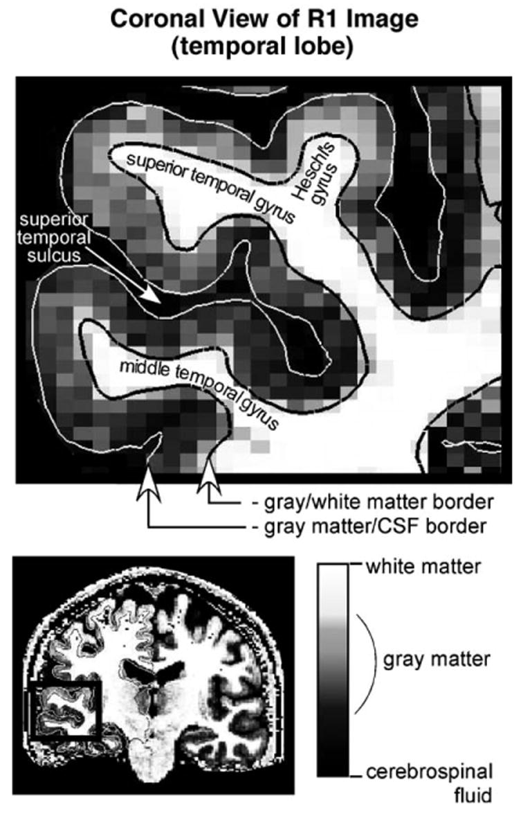
Coronal slice through the temporal lobe showing the spatial distribution of R1 at the resolution of the original images (1.3 × 1 × 1.3 mm). The grayscale value for each pixel indicates the magnitude of R1. White and black lines indicate the gray matter/CSF and gray matter/white matter borders, respectively, as determined by the segmentation procedure.

Gray matter R1 and thickness were estimated at points (spaced by ~1 mm) covering the cortical surface (i.e., the vertices of the surface). Thickness was estimated as the shortest distance between the CSF/gray matter and gray/white matter surfaces (Fischl and Dale, 2000). A single R1 value was obtained for each vertex by averaging R1 over this distance (Fischl et al., 2004). The averaging of R1 was across 80% of the depth of the gray matter starting from the gray/white matter border (Fig. 1, black line). 80% was used instead of 100% to exclude superficial R1 values that might represent a volume average of CSF and gray matter rather than purely gray matter. (Note, however, that the same qualitative results were obtained regardless of whether 80% or 100% was used.) A similar allowance for volume averaging was not made at the gray matter/white matter border because the potential for contamination was less (because the difference in R1 between gray matter and immediately underlying white matter is much less than the difference between gray matter and CSF (e.g., by approximately a factor of 4)).

Mapping and visualization

For each subject, gray matter R1 and thickness were mapped over the cortical surface and viewed on reconstructions of the temporal lobes (created from the segmented gray matter using FreeSurfer; Dale et al., 1999; Fischl et al., 1999). The maps were also viewed in a format that computationally inflates the cortex so that the cortical surface on gyri and in sulci could be viewed simultaneously (inflation performed using FreeSurfer). While this inflated representation is not used here for data presentation, it was helpful in forming an initial impression of the global variations in R1 over the temporal lobe. Note that all quantifications in this study were performed on the original, folded cortex.

When the R1 maps for each subject and hemisphere were thresholded to show only the highest R1 values on the temporal lobe, the threshold was defined in the narrow range of values (determined separately for each hemisphere) where the spatial extent of displayed R1 changed most abruptly. For all hemispheres, the threshold came out exceeding the minimum R1 value on the temporal lobe by 58–62% of the difference between minimum and maximum. (Threshold R1 was between 0.72 and 0.79 (1/s) depending on subject and hemisphere.) After thresholding, small (less than 50 mm²) isolated clusters of high R1 were removed. This latter step resulted in the rejection of only 3–6 clusters per hemisphere (all located on Heschl’s gyri and in planum temporale) and had only a minor effect on the maps.

For each hemisphere, regions of highest R1 identified with the thresholding procedure were compared with a published probabilistic atlas of koniocortex (available on-line at www.bic.mni.mcgill.ca/cytoarchitectonics; Morosan et al., 2001, Rademacher et al., 2001). The atlas was created by histologically localizing three subdivisions of koniocortex (TE1.0, TE1.1, and TE1.2) in the left and right hemispheres of twenty-seven postmortem brains, mapping the brains into a common coordinate system (MNI, Montreal Neurological Institute), and combining data across brains. Since the analysis software used in the present study (FreeSurfer) automatically mapped each brain into the same coordinates (MNI), an atlas probability value could be assigned to each surface vertex on the superior temporal lobe. (Note: While the atlas includes separate probability values for TE1.0, TE1.1 and TE1.2, we summed these values for the present analyses to obtain a probability value for each surface vertex corresponding to the entirety of koniocortex.) High R1 regions were compared with the atlas (1) visually, by overlaying displays of the atlas on mappings of R1 and, (2) quantitatively, by averaging the atlas probability values across all surface vertices within regions of high R1 (an estimate of overlap between high R1 and atlas).

Compensating for the correlation between thickness and curvature

To examine the relationship between gray matter thickness and the surface curvature of the cortex, we calculated a correlation coefficient r between the two using the local thickness and curvature (from FreeSurfer) for all vertices on the temporal lobe. Because the correlation was considerable (r = −0.56, mean across hemispheres), we also examined spatial maps of thickness after mathematically compensating for this correlation. This compensation was a rough attempt to separate thickness variations related to neuronal composition from variations related to mechanical distortions associated with cortical folding. The compensation was achieved by (1) modeling the relationship between thickness (T) and curvature C as T = C*k + b, (2) estimating k and b (separately for each temporal lobe) using a least square error fit to the thickness/curvature data, and (3) calculating a curvature compensated thickness for each vertex by subtracting C*k from the raw (i.e., uncompensated) thickness value.

Note that there was almost no correlation between R1 and curvature (r = 0.11, mean across hemispheres), so there was no reason to examine curvature-compensated R1.

Defining regions of interest (ROIs)

Regional differences in R1 and thickness were quantified using the following ROIs defined based on gross anatomical landmarks (Fig. 2): HGpm was defined as the posteromedial two-thirds of the first Heschl’s gyrus. HGal was the remaining antero-lateral one-third of the first Heschl’s gyrus. PT included the superior temporal cortex lateral and posterior to the transverse temporal sulcus. Posteriorly, it was limited by the vertical wall of the temporo-parietal cortex, and anteriorly, it extended to the antero-lateral limit of the most lateral Heschl’s gyrus (either first or second). AMAwas located antero-medial to Heschl’s gyrus. It was limited medially by the circular sulcus, and anteriorly by an imaginary line extending perpendicularly from the circular sulcus to the anterior limit of the first Heschl’s gyrus. HG2 was defined, when present, as a second most lateral Heschl’s gyrus. STS included all of the gray matter within the superior temporal sulcus (both upper and lower lips). STG was defined as the lateral face of the superior temporal lobe extending from the anterior to the posterior limit of the STS.

Fig. 2.

ROIs displayed on a 3D reconstruction of the right superior temporal lobe in one subject (#5). AMA: antero-medial area; HGal: antero-lateral aspect of first Heschl’s gyrus; HGpm: posteromedial aspect of first Heschl’s gyrus; HG2: second Heschl’s gyrus; PT: planum temporale.

Validity of the techniques

The present study used previously tested methods for gray matter segmentation, spatial mapping, and R1 and thickness estimation (Fischl and Dale, 2000, Rosas et al., 2002, Fischl et al., 2004). However, one difference compared to most previous work is that the gray matter segmentation was performed on data acquired using a FLASH imaging sequence, rather than sequences more typically used for segmentation (e.g., MPRAGE). In early analyses, we tried superimposing MPRAGE-based segmentations onto the FLASH data but found that this introduced inaccuracies in the calculated R1 values. The inaccuracies arose because image distortions (which occur in any MR image) are slightly different for FLASH and MPRAGE resulting in slight differences in the location of the gray matter borders in the two types of images. We concluded that accurate gray matter R1 values could best be obtained by estimating gray matter location in the same images used to calculate R1 (i.e., the FLASH images).

To ensure that gray matter segmentation from the FLASH data was reliable, we tested the quality of the segmentation as follows. First, the border between gray and white matter (as automatically estimated by FreeSurfer) was inspected for any deviations from what the authors would have defined manually. No deviations were found. Second, the contrast between gray and white matter was quantified and compared with the contrast in MPRAGE data taken during the same imaging session. This tissue contrast indicates the degree to which gray and white matter are distinguishable and thus provides an indirect indication of the quality of segmentation. Tissue contrast was quantified as image signal in gray matter divided by image signal in the immediately underlying white matter. For each hemisphere, this value was determined at thirty points distributed over each superior temporal lobe. The average across points was the final contrast value for a given hemisphere. Contrast in the MPRAGE images was assessed for each hemisphere the same way and at the same thirty points as for the FLASH data. In 5/10 hemispheres, tissue contrast in the FLASH data (1.2–1.6) differed by ~10% or less from the contrast in the MPRAGE data, indicating that the quality of the segmentation was comparable in the two datasets. In two hemispheres (subject 3, left and right), MPRAGE data were not available, but the tissue contrast in the FLASH data (~1.5) was above average and fell within the range of contrasts for MPRAGE data in other hemispheres. The remaining three hemispheres (subject 4, left; subject 5, left and right) differed from the others in showing lower contrast in the FLASH data (1.2–1.3) and a FLASH contrast that was 20–33% below the MPRAGE contrast. While these hemispheres showed lower contrast than the others, there was no reason to reject them from the analyses. Indeed, they generally showed the same variations in R1 (and thickness) across ROIs as the other hemispheres. However, the lower contrast (and potentially less accurate segmentation) may still have had some affect on the pattern of high R1 regions identified through thresholding. This is because segmentation quality is especially important in the identification of high R1 regions since even slight inaccuracies in local segmentation could create artifactual peaks in R1 that would then perturb the detailed pattern of high R1 identified through thresholding (without necessarily altering the gross pattern of high R1 or the overall R1 value for the ROI).

Results

Spatial variations in gray matter R1

Sample maps of gray matter R1 on the surface of the superior temporal plane are shown for the left and right hemispheres of one subject in Fig. 3. This subject is typical in that R1 was low, overall, on planum polare, intermediate on planum temporale and high on Heschl’s gyrus, particularly the posteromedial aspect. In addition to these gross spatial variations, all hemispheres also showed variations within regions. For instance, R1 showed a fairly progressive increase from anterior to posterior within planum polare and extending onto the anterior parts of Heschl’s gyrus. (Note that the maps in Fig. 3 have been thresholded to highlight the gross variations, making these finer variations less apparent.) Within planum temporale, R1 varied spatially, although in a patchy way.

Fig. 3.

Typical maps of gray matter R1 on the superior temporal lobe. The maps correspond to the left and right hemispheres of one subject. R1 is indicated in color on a red (low R1) to yellow (high R1) scale. An approximately isotropic Gaussian smoothing (kernel size: 2–2.5 mm) was applied for the purposes of this display. The distribution of R1 suggests that gray matter myelin content is generally least anteriorly (in planum polare), intermediate posteriorly (on planum temporale), and greatest on Heschl’s gyrus.

Quantitative comparisons of R1 across ROIs on the superior temporal lobe confirmed regional differences in R1 seen qualitatively in the maps (Fig. 4). For instance, R1 was lowest in AMA (located within planum polare; 10/10 hemispheres), greatest on Heschl’s gyri (i.e., in HGpm, HGal, or HG2; 10/10 hemispheres), and intermediate between these extremes in PT (planum temporale; 10/10 hemispheres). Among the ROIs on Heschl’s gyri, HGpm (corresponding to the posteromedial two-thirds of first Heschl’s gyrus) showed the highest R1, on average, although the difference compared to the other two ROIs (HGal, HG2) was not significant. HGpm (but not HGal or HG2) showed significantly greater R1 than any of the ROIs off Heschl’s gyri, i.e., AMA (P < 0.0001; paired t test), PT (P = 0.002), STG (P = 0.06) and STS (P < 0.0001). Thus, the ROI analysis confirmed a concentration of high R1 values on Heschl’s gyri, particularly within the posteromedial two-thirds of the first (i.e., most anterior) gyrus.

Fig. 4.

Mean gray matter R1 for different ROIs on the superior temporal lobe. Error bars indicate ± one standard error. Each of the ten hemispheres was treated as a separate data point.

Regions of high R1 on the superior temporal lobe

Fig. 5 displays maps of the regions of highest R1 on the superior temporal lobe. These regions were isolated by adjusting the threshold value of R1 (separately for each hemisphere) to coincide with the sharpest spatial gradients in R1 on the superior temporal plane, a procedure that resulted in a narrow range of thresholds across hemispheres (i.e., threshold R1 was ~60% of the difference between the minimum and maximum R1 on the temporal lobe). All hemispheres showed the following trends. High R1 regions were never seen in planum polare. Nor were they seen on the superior temporal gyrus, or within the superior temporal sulcus (not visible in Fig. 5). High R1 regions were always found on Heschl’s gyri. For instance, all hemispheres showed high R1 overlapping the posteromedial two-thirds of first Heschl’s gyrus (white in Fig. 5). In most cases, this overlapping high R1 formed a single, continuous region. However, in two cases (subjects2L, 4L), it consisted of two. Plots of average R1 vs. position along trajectories (green in Fig. 6A) through the antero-medial and posterolateral edges of the high R1 on Heschl’s gyrus (red and blue, respectively in Fig. 6A) confirmed a local and distinct elevation in R1 that rapidly gave way to lower R1 posterolaterally (Fig. 6B, left), and even lower R1 antero-medially (Fig. 6B, right).

Fig. 5.

Regions of high R1 on the superior temporal lobe. Each panel shows either the right (top) or left (bottom) superior temporal lobe of a given subject. High R1 regions are white if they overlap first Heschl’s gyrus and are shaded (with diagonal lines) if they do not. A dashed line separates three hemispheres in which the pattern of high R1 may be less accurate because of lower gray/white matter contrast. In the left hemisphere of subjects 3 and 5, there is one region of high R1 overlapping posteromedial Heschl’s gyrus that appears as two seemingly disconnected white patches, one on the gyrus, and the other just lateral to it. The connection between the two patches lies within Heschl’s sulcus. There were no regions of high R1 on the lateral face of the temporal lobe or completely hidden from view within sulci. Therefore, these displays show all high R1 regions on the superior temporal lobe.

Fig. 6.

R1 vs. position along trajectories through high R1 regions on Heschl’s gyrus. (A) View of the superior temporal lobe showing the approximate orientation of the trajectories (green arrows). The actual trajectories followed the cortical surface. Red and blue lines indicate the antero-medial and posterolateral edges (respectively) of the high R1 regions on Heschl’s gyrus. (B) R1 vs. position (i.e., surface vertex number) averaged across hemispheres and trajectories (four trajectories per hemisphere, each located at a different position along the length of Heschl’s gyrus). Data from the three hemispheres with potentially less accurate segmentation (to right of dashed line in Fig. 5) were not included. Prior to averaging, individual trajectories for the left panel in B were aligned relative to the posterolateral edge of the high R1 region (blue line). Individual trajectories for the right panel in B were aligned relative to the antero-medial edge (red line). The horizontal axes are colored green to highlight the fact that they correspond to the postero-lateral (B, left) and antero-medial (B, right) trajectories schematized in panel A. Gray background shading indicates that the plotted data lie outside the region of high R1 as defined by the thresholding procedure (see Methods). Each hemisphere was considered a data point in calculating the standard error of the mean (shading indicates ± one SEM). The spacing between vertices is approximately 1 mm. Note that the edges of the high R1 region (red and blue vertical lines in panel B) coincide with the sharpest spatial change in R1.

While all hemispheres had the aforementioned trends in common, there were also variations in the pattern of high R1 regions. The variations were somewhat greater for the three hemispheres with potentially less accurate segmentation (to right of dashed line in Fig. 5; see Methods). While these hemispheres show the same gross trends as the others, they may provide a less accurate view of the detailed distribution of high R1. Thus, we focus here on the seven remaining hemispheres (to left of dashed line). Among these remaining hemispheres, there were two main forms of variability. First, the high R1 overlapping the posteromedial aspect of first Heschl’s gyrus differed in extent and disposition (relative to Heschl’s gyrus) across hemispheres. Second, hemispheres differed in whether they showed high R1 regions in PT. This latter difference did not reflect differences in the degree of uniformity of R1 within PT but instead reflected differences in the amplitude of local R1 elevations. In other words, all hemispheres had a non-uniform R1 distribution within PT, but local elevations in R1 only exceeded threshold for some hemispheres (i.e., subjects 2L, 3L, 4R, 4L, 5R, 5L in Fig. 5).

Since the regions of high R1, like previous histological localizations of koniocortex, showed considerable overlap with Heschl’s gyrus, the high R1 regions were compared with the current best estimate of koniocortex location in imaged brains i.e., a histologically based atlas in which each voxel is assigned a value corresponding to the probability of coincidence with one of three koniocortical divisions (Morosan et al., 2001; Rademacher et al., 2001). When displayed on individual hemispheres, the regions of highest R1 on Heschl’s gyrus always fell completely within the regions of non-zero probability in the atlas, indicating that the edges of the high R1 regions never extended beyond the bounds of koniocortex defined histologically in the postmortem brains used for the atlas. To quantify the overlap between high R1 and the atlas, the average atlas probability within the high R1 regions on Heschl’s gyrus was calculated (i.e., within the white areas in Fig. 5). This overlap was 0.79 when averaged across hemispheres, indicating that the high R1 regions tended to overlap high probability parts of the atlas (i.e., parts most likely to coincide with koniocortex).

An attempt was made to isolate regions of low R1 (i.e., local minima in R1, instead of local maxima). As for the high R1 regions, we examined maps of R1 at progressively different thresholds but obtained a very different impression. When the maps were thresholded to reveal high R1 regions, the extent of displayed R1 changed abruptly within a small range of thresholds, indicating a sharp change in R1 at the edges of the high R1 regions. Similarly abrupt changes were not seen when the maps were progressively thresholded to extract the minima. In other words, our attempts to isolate regions of low R1 did not reveal distinct ‘‘islands’’ of low R1 analogous to the islands of high R1 described above.

Hemispheric differences

Hemispheric differences in gray matter R1 were identified by calculating an asymmetry index for each subject and ROI. In particular, for each ROI, the asymmetry index was equal to the difference between R1 on the left and right (averaged across ROI) divided by the sum (Fig. 7). For all ROIs, the mean across subjects asymmetry index was greater than zero, indicating greater R1 on the left. However, the degree of asymmetry differed across ROIs with PT and STS showing the strongest asymmetry (index >0 in 5/5 subjects; P < 0.008 for each ROI based on a paired t test comparison of left and right R1 values), and HGpm and STG showing a lesser asymmetry (index >0 in 4/5 subjects; P = 0.05 for both ROIs). HGal and AMA did not show a significant asymmetry (P > 0.7). Thus, while gray matter R1 was generally greater on the left compared to the right, the asymmetry was most prominent in posterior regions of the superior temporal plane (PT, HGpm), on the STG, and within the STS.

Fig. 7.

Degree of R1 asymmetry on the superior temporal lobe. For each ROI and subject, an asymmetry index was calculated as the difference in R1 between the left and right sides divided by the sum. Each black circle indicates the index for a particular subject. Gray bars indicate the mean across subjects. Dashed horizontal line at zero indicates no asymmetry. HGpm, PT, STG, and STS showed significant asymmetry whereas ROIs located anteriorly on the superior temporal plane (AMA, HGal) did not (based on a statistical comparison of left vs. right R1 values; paired t test). No data are given for HG2 since none of the subjects had a second Heschl’s gyrus on both the left and right sides.

Spatial variations in gray matter thickness

Gray matter thickness (obtained secondarily from the R1 analyses) was generally greater on the temporal lobe than in other parts of the cortex. Within the superior temporal lobe, thickness varied spatially in two ways. First, it tended to increase toward the temporal pole. Second, it tended to vary in accordance with the sulcal/gyral patterns of the cortex (von Economo, 1929). The latter trend is illustrated by the thinner gray matter of sulcal regions AMA, PT, and STS as compared to gyral regions HGal and STG (Fig. 8A). It is also reflected in the correlation between thickness and the surface curvature of the cortex (r = −0.56; average across hemispheres).

Fig. 8.

Left: Mean gray matter thickness for different ROIs on the superior temporal lobe. Right: Same as left panel except thickness has been compensated for curvature. Error bars indicate ± one standard error. Each of the 10 hemispheres was treated as a separate data point.

To identify any regional variations in thickness unrelated to curvature, the correlation between thickness and curvature was compensated for mathematically. After compensation, thickness no longer differed significantly between most cortical regions (Fig. 8B). The exception was AMA, which showed a significantly greater curvature-corrected thickness (P < 0.008; paired t test).

To examine whether auditory cortical areas can be delineated in any way using gray matter thickness information, gray matter thickness maps (compensated for curvature) were gradually thresholded to isolate either the thickest or thinnest cortex in the temporal lobe. However, a consistent pattern of local maxima (high thickness regions) or local minima (low thickness regions) did not emerge from this analysis, except for a region of high thickness at the temporal pole resulting from the global trend of gray matter thickening from posterior to anterior.

There was no hemispheric difference in gray matter thickness for any ROI either before or after the compensation for curvature (P > 0.4 in left/right comparison of each ROI).

Discussion

The present study mapped the spatial patterns of gray matter R1 over the surface of the temporal lobe in living humans. Cross-regional variations revealed by these mappings were highly repeatable across subjects. For instance, R1 was always lowest overall on planum polare, intermediate on planum temporale and high on Heschl’s gyri. When the R1 maps were thresholded to isolate regions of highest R1, such regions were always found overlapping posteromedial Heschl’s gyrus. They also sometimes occurred in planum temporale, although not in any other part of the superior temporal lobe. Comparisons of R1 between hemispheres also showed repeatable trends, namely systematically greater R1 on the left in posterior parts of the superior temporal plane, as well as STG and STS. To our knowledge, this is one of the first studies to have analyzed spatial mappings of intrinsic MR properties of the gray matter (Fischl et al., 2004), and the only such study directed at auditory cortex.

R1 and gray matter myelination

While the basis for inter-regional differences in gray matter R1 is a matter of some debate (e.g., Gelman et al., 2001; Steen et al., 2000), there are several indications that the regional variations in the present study predominantly reflect variations in myelin content. Biophysical experiments in aqueous solutions containing controlled solutes have shown that myelin (or more specifically the cholesterol of myelin) is a potent facilitator of longitudinal relaxation, producing substantial increases in R1 (and hence high signal in the white matter of R1-weighted images; Koenig et al., 1990). Measurements of gray matter R1 in children have shown increases with age that coincide with the increase in neuronal myelination that occurs during development (Moore and Guan, 2001; Steen and Schroeder, 2003). R1 and myelin content have shown high correlation in spinal cord samples from multiple sclerosis patients (Mottershead et al., 2003). The patterns of R1 in the present study themselves suggest a relationship between R1 and myelin. For instance, Heschl’s gyri have been described as one of the most heavily myelinated areas of the temporal lobe (Hopf, 1968; Hackett et al., 2001; Wallace et al., 2002) in agreement with the elevation in R1 seen in this region. In addition, areas lateral and posterior to Heschl’s gyrus have been described as less heavily myelinated while cortex antero-medial to Heschl’s gyrus has been described as only sparsely myelinated (Hopf, 1968; Hackett et al., 2001; Wallace et al., 2002), observations that follow the trends in gray matter R1 reported here. Additional evidence indicating a strong myelin contribution to R1 comes from a recent study showing that the laminar distribution of R1 in gray matter corresponds more closely to the distribution of myelin than to the distribution of cell bodies (Eickhoff et al., 2005). Thus, there is a variety of evidence to support a strong relationship between R1 and myelin content in cortical gray matter.

While there is clear evidence that myelin content has a major influence on inter-regional variations in gray matter R1, we cannot rule out contributions from other factors (Steen et al., 2000; Vymazal et al., 1999; Gelman et al., 2001). Indeed, a sole dependence on myelin seems unlikely given the complex biophysical processes underlying R1 (Gore and Kennan, 1999). Some of the other possible contributors (e.g., water content, axonal density) may correlate with myelin and thus may not be true independent factors (Mottershead et al., 2003). However, others, such as non-heme iron, may affect R1 independently especially in pathological brains (e.g., Alzheimer’s disease). At present, there is no conclusive evidence for or against an important non-myelin-related contribution to the inter-regional variations in R1 in normal cerebral cortex. Therefore, given the evidence at hand, we interpret the spatial variations in R1 seen in the present study as variations in gray matter myelin content, recognizing that this interpretation requires further testing.

High R1 on Heschl’s gyrus: a marker for koniocortex?

The high R1 found overlapping posteromedial Heschl’s gyrus in every hemisphere bears several similarities to auditory koniocortex (i.e., Brodmann area 41; Campbell, 1905; von Economo, 1929; Hopf, 1968; Galaburda and Sanides, 1980; Rademacher et al., 1993; Rivier and Clarke, 1997; Morosan et al., 2001; Rademacher et al., 2001; Hackett et al., 2001; Wallace et al., 2002; Sweet et al., 2005). First, this high R1 always shared the same general location as koniocortex, i.e., the posteromedial two-thirds of Heschl’s gyrus. The similarity in location can be seen by comparing the white R1 regions in Fig. 5 with histologically localized koniocortex in Fig. 2 of Rademacher et al. (2001). It is also apparent from the complete overlap found between high R1 on Heschl’s gyrus and the probabilistic atlas of Rademacher et al. (2001). Second, koniocortex is an area of especially heavy myelination (Hopf, 1968; Galaburda and Sanides, 1980; Hackett et al., 2001; Wallace et al., 2002), and so, presumably, are regions of high R1. Finally, the heavy myelination of koniocortex rapidly gives way to lower myelination medially and, to a lesser extent, laterally (Hopf, 1968; Hackett et al., 2001; Wallace et al., 2002). Correspondingly, the limiting borders of high R1 were defined to coincide with abrupt spatial changes in R1. Thus, the position of the high R1 regions, their interpretation as areas of heavy gray matter myelination, and the abruptness of their borders leads to the following hypothesis: the high R1 overlapping posteromedial Heschl’s gyrus (the more anterior gyrus when there are two) corresponds, in whole or in part, to auditory koniocortex.

In some hemispheres, more than one high R1 region was isolated on the superior temporal plane (see Fig. 5). In these cases, only the regions overlapping the posteromedial part of first Heschl’s gyrus can be reasonably hypothesized to correspond to koniocortex. The remaining high R1 regions (confined to planum temporale) can be confidently rejected as correlates of koniocortex since their position is unequivocally inconsistent with previous histological localizations of koniocortex on the superior temporal plane. We suggest that the high R1 regions within planum temporale reflect inhomogeneities in gray matter myelination of this area. Such inhomogeneities would have been difficult to discern in previous histological studies, which did not include continuous, spatial mappings of gray matter myelin content. Inhomogeneities (local elevations in R1) occurred in every planum but were only apparent in some of the cases in Fig. 5 because the amplitude of local elevations in R1 varied across subjects and only exceeded threshold R1 in some hemispheres. In other words, all hemispheres showed inhomogeneities in the distribution of gray matter R1 in planum temporale. These likely reflect the architectonic diversity of this area.

While the present data are promising in suggesting that auditory koniocortex can be identified by isolating regions of high R1, they also suggest that further work may be needed to develop R1 into a definitive marker for koniocortex. While the extent and location of koniocortex varies across subjects and hemispheres (e.g., see Fig. 2 of Rademacher et al., 2001) and the high R1 regions overlapping Heschl’s gyrus show a comparable degree of variability, some of the precise variants in the R1 data have no counterpart in the anatomical literature. For instance, in subject 3L, the high R1 region overlapping Heschl’s gyrus spreads well into planum temporale and, in subject 2L, the high R1 on Heschl’s gyrus is split in two (Fig. 5).¹ In future work, it will be important to determine how closely high R1 regions correspond to koniocortex as it would be defined histologically and, if necessary, refine the criteria for defining the limiting borders of high R1. Here, the borders of high R1 were adjusted to coincide with the most abrupt spatial changes in R1. However, it is possible that a different criterion would yield a better coincidence with the true borders of koniocortex.

Using high-resolution imaging of the laminar structure of the gray matter, it should be possible to examine the relationship between high R1 regions and koniocortex, and perhaps refine the defining criteria for high R1 borders so as to maximize this correspondence. By pushing the resolving power of MRI, it is possible to obtain, in vivo, images of gray matter laminar structure showing detail comparable to low-magnification microscopic images of myelin-stained tissue (Barbier et al., 2002; Walters et al., 2003). By obtaining such images and R1 mappings in the same subjects, it should be possible to compare the laminar pattern of myelination of gray matter within vs. outside regions of high R1. In particular, it should be possible to determine whether regions of high R1 show the dense myelination of lower gray matter layers characteristic of koniocortex and whether the density of myelination in the lower layers lessens laterally to make the bands of myelination in layers IV and V, characteristic of the lateral belt, appear more prominently (e.g., Hackett et al., 2001). It should be noted that high-resolution imaging of gray matter laminar structure is not a replacement for R1 mapping. Advantages of R1 mapping include speed and simplicity, important attributes for the applications discussed below (see Significance and implications).

Because of the absence of physiological noise and the possibility of prolonged scanning, ex vivo imaging of the gray matter offers the possibility of increased spatial resolution and/or signal-to-noise compared to in vivo imaging. Therefore, using ex vivo imaging to test the correspondence between high R1 and koniocortex would be ideal were it not for a technical issue: R1 is substantially increased in fixed tissue making its reliable estimation difficult (Gore and Kennan, 1999). Still, other intrinsic MR parameters that correlate with myelin content equally well (e.g., magnetization transfer ratio) can be measured in postmortem tissue and could be examined in lieu of R1 (Mottershead et al., 2003; Schmierer et al., 2004). Measurements of magnetization transfer ratio might be particularly advantageous since they can be made both in vivo and ex vivo.

The degree of correspondence between high R1 and koniocortex could also be tested by comparing R1 and tonotopic mappings in the same subjects. The koniocortex of non-human primates contains mirror-image spatial maps of frequency sensitivity (e.g., Kaas et al., 1999) and, a similar arrangement of tonotopic mappings has been described on Heschl’s gyri in humans (Formisano et al., 2003; Schönwiesner et al., 2002; Talavage et al., 2000, 2004). A demonstration of mirror-image tonotopic mappings within regions of high R1 on posteromedial Heschl’s gyrus would provide functional corroboration that the high R1 corresponds to koniocortex.

The fact that high R1 was found overlapping posteromedial Heschl’s gyrus in every subject and hemisphere studied indicates that an R1-based marker for koniocortex, refined and tested as just described, would be applicable to individuals. This is highly significant for studies attempting to relate cortical function to structure since auditory koniocortex, like other architectonic areas, varies across subjects in its relationship to the gross anatomy of the cerebrum (Rademacher et al., 2001). Therefore, without a means of identifying koniocortex directly in functionally imaged subjects, one is left to approximate its location using mappings into normalized coordinates, into surface-based coordinates, or onto probabilistic atlases (Talairach and Tournoux, 1988; Fischl et al., 1999; Rademacher et al., 2001). At present, there is no established in vivo marker for auditory koniocortex, anatomic or physiologic. In contrast to the retinotopic mappings used to distinguish fields of visual cortex, tonotopic mappings have proved difficult to obtain and are not yet routinely measured. While not in routine use at present, the spatiotemporal patterns of BOLD response in auditory cortex may provide a robust, physiologic means for distinguishing auditory cortical areas (Seifritz et al., 2002; Harms et al., 2005) in fMRI studies, and this could complement the anatomic R1 mapping approach of the present study.

Hemispheric differences and functional interpretations

Our finding of a left–right difference in gray matter R1 is a new observation that adds to a wealth of previous data documenting hemispheric differences in gross morphology or gray matter microstructure of the posterior temporal plane and Heschl’s gyri (gross morphology: Geschwind and Levitsky, 1968; Galaburda et al., 1978; Penhune et al., 1996; Leonard et al., 1998; microstructure: Seldon, 1981a,b, 1982, Hutsler and Gazzaniga, 1996; Anderson et al., 1999; Galuske et al., 2000; Buxhoeveden et al., 2001). The present R1 data complement this previous work by indicating a left–right difference in the myelination of the gray matter of the temporal lobe and doing so in living humans.

While the previous work on asymmetries of the temporal lobe does not report an asymmetry in gray matter myelination, it does provide data consistent with this trend (see Zatorre et al., 2002). For instance, Penhune et al. (1996) showed that the volume of the gray matter on first Heschl’s gyrus is similar on the left and right, whereas the volume of the underlying white matter is greater on the left. If this greater white matter volume reflects a larger number and/or caliber of myelinated fibers that continues into the overlying gray matter, it would contribute to greater overall myelin content within the gray matter of left Heschl’s gyrus. The volumetric data of Anderson et al. (1999) suggest a similar picture within the portion of the superior temporal lobe posterior to Heschl’s gyrus. Thus, while the present study provides the most direct indication to date that gray matter myelination is greater in the left temporal lobe (as compared to the right), there are previous data to support this observation.

An asymmetry in gray matter myelination is directly relevant to proposals that the left hemisphere is preferentially involved in the processing of rapid temporal changes in acoustic signals. These proposals come from studies of brain function using various techniques. For example, deficits in rapid temporal processing have been observed in patients with left, but not right temporal lobe lesions (Efron, 1963; Robin et al., 1990; Ehrle et al., 2001). In normal subjects, greater PET activation on the left Heschl’s gyrus was observed for tasks that tested subject’s ability to process rapid changes in the temporal aspects of non-speech sounds, while greater activation on the right side was observed for tasks that tested subject’s ability to process rapid changes in pitch (Zatorre and Belin, 2001). Intracerebral recordings in epilepsy patients showed that left temporal regions are able to follow temporal transitions in speech and non-speech sounds better than right temporal regions (Liégeois-Chauvel et al., 1999). Our data indicating hemispheric differences in gray matter R1 and, by extension, myelination suggest a structural substrate for the functional findings. Since myelin plays a crucial role in maintaining the timing of neural activity, greater myelination on the left could increase the precision of neural timing, thus providing the left hemisphere with an enhanced ability (over the right) to discriminate and follow rapid acoustic changes.

The gray matter asymmetry observed in the present study may also play a role in the left hemispheric specialization for speech and language in humans. The reasons for suggesting this are two-fold. First, the observation of greater gray matter R1 on the left was only seen in regions of the temporal lobe heavily implicated in language processing (PT, STG, STS) (Zatorre et al., 1992; Binder et al., 2000; Hickok and Poeppel, 2000) or in regions supplying inputs (directly or indirectly) to those more specialized regions (HGpm; Kaas et al., 1999). Second, behavioral studies in clinical populations have indicated that accurate temporal processing may be crucial to normal speech and language functions (Efron, 1963; Robin et al., 1990; Tallal, 1980a, Tallal and Stark, 1981). Thus, a leftward bias in gray matter myelination, if it is indeed a substrate for higher fidelity temporal processing, may by extension be an important substrate for the left-hemispheric specialization for speech and language.

Gray matter thickness: new observations and comparisons with previous data

The thickness of gray matter on the temporal lobe showed consistent trends across subjects, some noted previously. Consistent with the well-documented fact that the gray matter of gyri is thicker than that of sulci (von Economo, 1929; Blinkov and Glezer, 1968), we found that thickness correlated with the surface curvature of temporal cortex, as have previous MR imaging studies (Kang et al., 2003). In keeping with previous observations by von Economo (1929), gray matter thickness was generally greater on the temporal lobe than in the rest of the cerebrum (see also Fischl and Dale, 2000) and tended to increase from posterior to anterior toward the temporal pole. Values for auditory gray matter thickness based on histology are in approximate agreement with the present study, but tend to run slightly greater (~3 mm, von Economo, 1929). The difference may reflect the overestimation inherent in measuring thickness from 2D slices of tissue (e.g., as von Economo did), rather than in 3D (as in the present study). In 2D slices, much of the gray matter will be intersected obliquely, resulting in a systematic overestimation of thickness.

We examined whether thickness maps might be used to isolate cortical areas in the same way that R1 maps were, but the results were not promising. Thresholding the thickness maps did not reveal circumscribed regions of either high or low thickness, even when the maps were adjusted to compensate for the correlation between thickness and cortical curvature, a correlation that might overwhelm other spatial variations in thickness related to differences in neuronal composition (e.g., neuronal size or number) between cortical areas.

While gray matter thickness may not be useful for delineating auditory cortical areas, it may still prove informative in studies of auditory cortex. Gray matter thickness is known to change with learning, development, and sensory deprivation (Argandona and Lafuente, 1996; O’Kusky and Colonnier, 1982; Anderson et al., 2002). It would be interesting to see whether changes also occur during, e.g., language acquisition, auditory training, or following damage to the auditory periphery—and whether they occur differentially between cortical regions.

Comparison to previous histological work

The present work, while in agreement with the pertinent histological data on gray matter myelination and thickness, provides very different information concerning gray matter structure on the human temporal lobe. The previous observations in histological tissue were generally qualitative and were based on discrete samples of the cortex, either closely spaced histological sections limited to subregions of the temporal lobe (Hackett et al., 2001; Wallace et al., 2002) or sparse samples over large expanses of the temporal lobe (Hopf, 1968). The methods of the present study, by contrast, provide a near-continuous assessment of gray matter myelination (indirectly via R1) and thickness that is at once quantitative and inclusive of the entire temporal lobe.

Technical issues and future improvements

Since the accuracy of gray matter segmentation is important to achieving reliable R1 mappings, it is worth mentioning methods that might yield greater segmentation accuracy by increasing the ratio between gray/white matter contrast and image noise. These include using a multi-echo sequence instead of multiple single echo sequences, using multi-channel array coils, and acquiring more data per subject. The latter approach would entail longer scan times, but this could be offset by imaging only the regions of interest instead of the entire brain.

Even with improvements in segmentation quality, the accuracy of segmentation is likely to vary between gray matter areas because of regional differences in anatomy. For instance, the heavily myelinated lower layers of koniocortical gray matter are more likely to be lumped with underlying white matter than are the less myelinated lower layers of adjacent gray matter areas. We cannot rule out that some mis-assignment of the lower layers occurred in the present study. However, if it did, it would have resulted in a selective underestimation of R1 in koniocortex, an effect that would have worked against obtaining one of the main results of this study (i.e., high R1 overlapping posteromedial Heschl’s gyrus and putatively corresponding to koniocortex). Improvements in segmentation (to prevent mis-assignment of the lower koniocortical layers) should, if anything, make this result more robust.

Significance and implications

The present analysis of R1 in auditory cortex provides a proof of concept for delineating cortical divisions, both auditory and non-auditory, based on mappings of gray matter MR tissue properties. Delineation of cortical areas by mapping such properties (or MR signal intensity) over the gray matter sheet has been proposed before (Rebmann and Butman, 2003). In addition, differences in some MR properties between gross regions of interest in the gray matter have been reported (e.g., between HG and STG, Yoshiura et al., 2000; see also Besson et al., 1989; Steen et al., 2000). However, to our knowledge, the present study represents the first attempt to localize an architectonic area based on spatial mapping of an intrinsic gray matter variable. Importantly, the results are promising.

Being able to delimit auditory koniocortex and perhaps, eventually, other architectonic areas directly in individual, living humans should enable new advances in our understanding of the relationship between cortical structure and function. Since the position of architectonic divisions varies across subjects (e.g., Rademacher et al., 1993) and methods for identifying these divisions directly in living humans have been lacking, functional neuroimaging data have generally been related to cortical architectonics by approximate means, i.e., mapping probabilistic atlases of cortical architectonics onto the functionally imaged brains, or mapping these brains into a normalized space so that Brodmann areas can be assigned (Talairach and Tournoux, 1988; Fischl et al., 1999; Rademacher et al., 2001). Delimiting architectonic divisions of the cortex directly in individual subjects who are also functionally imaged would allow cortical structure and function to be compared directly on an individual basis, perhaps revealing correspondences previously obscured because of approximations in architectonic location.

Having markers for architectonic divisions of auditory cortex, and koniocortex in particular, is especially significant because there is currently no established way to differentiate auditory areas – structurally or functionally – in living humans. Retinotopic mappings are routinely used to subdivide the human visual cortex, providing a reference for interpreting additional functional data (e.g., Sereno et al., 1995). In auditory cortex, however, there is no corresponding reference. The results of the present study indicate that R1 mappings might provide one such reference, i.e., a ‘‘koniocortex localizer’’. Routinely adding such a reference scan to auditory fMRI studies should be feasible given the fairly short scan time for R1 mapping.

While providing new data in normal, adult subjects, the present study also lays a groundwork for investigations of auditory gray matter structure in other populations and contexts. For instance, changes in gray matter myelination that occur in auditory cortex over the first two decades of life (e.g., Moore and Guan, 2001) could be tracked and understood in ways not possible from limited amounts of histological material. Given the crucial role for myelin in maintaining the timing of neural activity, it may prove illuminating to examine the R1 patterns of individuals with auditory temporal processing deficits (e.g., as reportedly occur with dyslexia; Tallal, 1980b). More generally, insights into the structural substrates behind human hearing and speech perception might be obtained by assessing gray matter structural variables in patients with auditory psychophysical deficits or communication disorders. Overall, there are many additional lines of investigation suggested by the approach of the present study; the findings here are only an initial demonstration of the things to be learned by spatially mapping intrinsic gray matter properties in living humans.

References

- Anderson B, Southern BD, Powers RE. Anatomic asymmetries of the posterior superior temporal lobes: a postmortem study. Neuropsychiatry Neuropsychol Behav Neurol. 1999;12:247–254. [PubMed] [Google Scholar]
- Anderson BJ, Eckburg PB, Relucio KI. Alterations in the thickness of motor cortical subregions after motor-skill learning and exercise. Learn Mem. 2002;9:1–9. doi: 10.1101/lm.43402. [DOI] [PMC free article] [PubMed] [Google Scholar]
- Argandona EG, Lafuente JV. Effects of dark-rearing on the vascularization of the developmental rat visual Cortex. Brain Res. 1996;732:43–51. doi: 10.1016/0006-8993(96)00485-4. [DOI] [PubMed] [Google Scholar]
- Barbier EL, Marrett S, Danek A, Vortmeyer A, van Gelderen P, Duyn J, Bandettini P, Grafman J, Koretsky AP. Imaging cortical anatomy by high-resolution MR at 3.0 T: detection of the stripe of Gennari in visual area 17. Magn Reson Med. 2002;48:735–738. doi: 10.1002/mrm.10255. [DOI] [PubMed] [Google Scholar]
- Besson JAO, Greentree SG, Foster MA, Rimmington JE. Regional variation in rat brain proton relaxation times and water content. Magn Reson Imaging. 1989;7:141–143. doi: 10.1016/0730-725x(89)90696-6. [DOI] [PubMed] [Google Scholar]
- Binder JR, Frost JA, Hammeke TA, Bellgowan P, Springer JA, Kaufman JN, Possing ET. Human temporal lobe activation by speech and nonspeech sounds. Cereb Cortex. 2000;10:512–528. doi: 10.1093/cercor/10.5.512. [DOI] [PubMed] [Google Scholar]
- Blinkov S, Glezer I. The Human Brain in Figs. and Tables: A Quantitative Handbook. Basic Books; New York: 1968. [Google Scholar]
- Brodmann K. Brodmann’s ‘‘Localisation in the Cerebral Cortex’’. Smith-Gordon; London: 1909. [Google Scholar]
- Buxhoeveden DP, Switala AE, Litaker M, Roy E, Casanova MF. Lateralization of minicolumns in human planum temporale is absent in nonhuman primate cortex. Brain Behav Evol. 2001;57:349–358. doi: 10.1159/000047253. [DOI] [PubMed] [Google Scholar]
- Campbell AW. Histological Studies on the Localization of Cerebral Function. Cambridge Univ. Press; Cambridge: 1905. [Google Scholar]
- Dale AM, Fischl B, Sereno MI. Cortical surface-based analysis: I. Segmentation and surface reconstruction. NeuroImage. 1999;9:179–194. doi: 10.1006/nimg.1998.0395. [DOI] [PubMed] [Google Scholar]
- Draganski B, Gaser C, Busch V, Schuierer G, Bogdahn U, May A. Neuroplasticity: changes in grey matter induced by training. Nature. 2004;427:311–312. doi: 10.1038/427311a. [DOI] [PubMed] [Google Scholar]
- Efron R. Temporal perception, Aphasia and D’ej’a Vu. Brain. 1963;86:403–424. doi: 10.1093/brain/86.3.403. [DOI] [PubMed] [Google Scholar]
- Ehrle N, Samson S, Baulac M. Processing of rapid auditory information in epileptic patients with left temporal lobe damage. Neuropsychologia. 2001;39:525–531. doi: 10.1016/s0028-3932(00)00121-4. [DOI] [PubMed] [Google Scholar]
- Eickhoff S, Walters NB, Schleicher A, Kril J, Egan GF, Zilles K, Watson JDG, Amunts K. High-resolution MRI reflects myeloarchitecture and cytoarchitecture of human cerebral cortex. Hum Brain Mapp. 2005;24:206–215. doi: 10.1002/hbm.20082. [DOI] [PMC free article] [PubMed] [Google Scholar]
- Fischl B, Dale AM. Measuring the thickness of the human cerebral cortex from magnetic resonance images. Proc Natl Acad Sci. 2000;97:11050–11055. doi: 10.1073/pnas.200033797. [DOI] [PMC free article] [PubMed] [Google Scholar]
- Fischl B, Sereno MI, Dale AM. Cortical surface-based analysis: II. Inflation, flattening, and a surface-based coordinate system. Neuro-Image. 1999;9:195–207. doi: 10.1006/nimg.1998.0396. [DOI] [PubMed] [Google Scholar]
- Fischl B, Salat DH, van der Kouwe AJW, Makris N, Ségonne F, Quinn BT, Dale AM. Sequence-independent segmentation of magnetic resonance images. NeuroImage. 2004;23:S69–S84. doi: 10.1016/j.neuroimage.2004.07.016. [DOI] [PubMed] [Google Scholar]
- Formisano E, Kim DS, Di Salle F, van de Moortele PF, Ugurbil K, Goebel R. Mirror-symmetric tonotopic maps in human primary auditory cortex. Neuron. 2003;40:859–869. doi: 10.1016/s0896-6273(03)00669-x. [DOI] [PubMed] [Google Scholar]
- Galaburda A, Sanides F. Cytoarchitectonic organization of the human auditory cortex. J Comp Neurol. 1980;190:597–610. doi: 10.1002/cne.901900312. [DOI] [PubMed] [Google Scholar]
- Galaburda AM, LeMay M, Kemper TL, Geschwind N. Right–left asymmetrics in the brain. Science. 1978;199:852–856. doi: 10.1126/science.341314. [DOI] [PubMed] [Google Scholar]
- Galuske RA, Schlote W, Bratzke H, Singer W. Interhemispheric asymmetries of the modular structure in human temporal cortex. Science. 2000;289:1946–1949. doi: 10.1126/science.289.5486.1946. [DOI] [PubMed] [Google Scholar]
- Gelman N, Ewing JR, Gorell JM, Spickler EM, Soloman EG. Interregional variation of longitudinal relaxation rates in human brain at 3.0 T: relation to estimated iron and water contents. Magn Res Med. 2001;45:71–79. doi: 10.1002/1522-2594(200101)45:1<71::aid-mrm1011>3.0.co;2-2. [DOI] [PubMed] [Google Scholar]
- Geschwind N, Levitsky W. Human brain: left–right asymmetries in temporal speech region. Science. 1968;161:186–187. doi: 10.1126/science.161.3837.186. [DOI] [PubMed] [Google Scholar]
- Gore JC, Kennan RP. Physical and physiological basis of magnetic relaxation. In: Stark DD, Bradley WG Jr, editors. Magn Reson Imaging. Vol. 1. Mosby; St. Louis: 1999. pp. 33–42. [Google Scholar]
- Hackett TA, Preuss TM, Kaas JH. Architectonic identification of the core region in auditory cortex of macaques, chimpanzees, and humans. J Comp Neurol. 2001;441:197–222. doi: 10.1002/cne.1407. [DOI] [PubMed] [Google Scholar]
- Harms MP, Guinan JJ, Jr, Sigalovsky IS, Melcher JR. Shortterm sound temporal envelope characteristics determine multisecond time patterns of activity in human auditory cortex as shown by fMRI. J Neurophysiol. 2005;93:210–222. doi: 10.1152/jn.00712.2004. [DOI] [PubMed] [Google Scholar]
- Hickok G, Poeppel D. Towards a functional neuroanatomy of speech perception. Trends Cogn Sci. 2000;4:131–138. doi: 10.1016/s1364-6613(00)01463-7. [DOI] [PubMed] [Google Scholar]
- Hopf A. Photometric studies on the myeloarchitecture of the human temporal lobe. J Hirnforsch. 1968;10:285–297. [PubMed] [Google Scholar]
- Hutsler JJ, Gazzaniga MS. Acetylcholinesterase staining in human auditory and language cortices: regional variation of structural features. Cereb Cortex. 1996;6:260–270. doi: 10.1093/cercor/6.2.260. [DOI] [PubMed] [Google Scholar]
- Kaas JH, Hackett TA, Tramo MJ. Auditory processing in primate cerebral cortex. Curr Opin Neurobiol. 1999;9:164–170. doi: 10.1016/s0959-4388(99)80022-1. [DOI] [PubMed] [Google Scholar]
- Kang X, Yund B, Woods D. Cortical thickness measurements of human auditory cortex. Abstracts for the International Society for Magnetic Resonance in Medicine.2003. [Google Scholar]
- Koenig SH, Brown RD, III, Spiller M, Lundbom N. Relaxometry of brain: why white matter appears bright in MRI. Magn Reson Med. 1990;14:482–495. doi: 10.1002/mrm.1910140306. [DOI] [PubMed] [Google Scholar]
- Leonard CM, Voeller KKS, Lombardino LJ, Morris MK, Hynd GW, Alexander AW, Andersen HG, Garofalakis M, Honeyman JC, Mao J, Agee OF, Staab EV. Anomalous cerebral structure in dyslexia revealed with magnetic resonance imaging. Arch Neurol. 1993;50 (5):461–469. doi: 10.1001/archneur.1993.00540050013008. [DOI] [PubMed] [Google Scholar]
- Leonard CM, Puranik C, Kuldau JM, Lombardino LJ. Normal variation in the frequency and location of human auditory cortex landmarks. Heschl’s gyrus: where is it? Cereb Cortex. 1998;8:397–406. doi: 10.1093/cercor/8.5.397. [DOI] [PubMed] [Google Scholar]
- Liégeois-Chauvel C, de Graaf JB, Laguitton V, Chauvel P. Specialization of left auditory cortex for speech perception in man depends on temporal coding. Cereb Cortex. 1999;9:484–496. doi: 10.1093/cercor/9.5.484. [DOI] [PubMed] [Google Scholar]
- MacDonald D, Kabani N, Avis D, Evans AC. Automated 3-D extraction of inner and outer surfaces of cerebral cortex from MRI. NeuroImage. 2000;12:340–356. doi: 10.1006/nimg.1999.0534. [DOI] [PubMed] [Google Scholar]
- Moore JK, Guan YL. Cytoarchitectural and axonal maturation in human auditory cortex. JARO. 2001;2:297–311. doi: 10.1007/s101620010052. [DOI] [PMC free article] [PubMed] [Google Scholar]
- Morosan P, Rademacher J, Schleicher A, Amunts K, Schormann T, Zilles K. Human primary auditory cortex: cytoarchitectonic subdivisions and mapping into a spatial reference system. NeuroImage. 2001;13:684–701. doi: 10.1006/nimg.2000.0715. [DOI] [PubMed] [Google Scholar]
- Mottershead JP, Schmierer K, Clemence M, Thornton JS, Scaravilli F, Barker GJ, Tofts PS, Newcombe J, Cuzner ML, Ordidge RJ, McDonald WE, Miller DH. High field MRI correlates of myelin content and axonal density in multiple sclerosis—A post-mortem study of the spinal cord. J Neurol. 2003;250:1293–1301. doi: 10.1007/s00415-003-0192-3. [DOI] [PubMed] [Google Scholar]
- Narr KL, Toga AW, Szeszko P, Thompson PM, Woods RP, Robinson D, Sevy S, Wang Y, Schrock K, Bilder RM. Cortical thinning in cingulated and occipital cortices in first episode schizophrenia. Biol Psychiatry. 2005;58:32–40. doi: 10.1016/j.biopsych.2005.03.043. [DOI] [PubMed] [Google Scholar]
- Nishimura DG. Principles of Magnetic Resonance Imaging 1996 [Google Scholar]
- O’Kusky J, Colonnier M. Postnatal changes in the number of neurons and synapses in the visual cortex (area 17) of the macaque monkey: a stereological analysis in normal and monocularly deprived animals. J Comp Neurol. 1982;210:291–306. doi: 10.1002/cne.902100308. [DOI] [PubMed] [Google Scholar]
- Penhune VB, Zatorre RJ, MacDonald JD, Evans AC. Interhemispheric anatomical differences in human primary auditory cortex: probabilistic mapping and volume measurement from magnetic resonance scans. Cereb Cortex. 1996;6:661–672. doi: 10.1093/cercor/6.5.661. [DOI] [PubMed] [Google Scholar]
- Rademacher J, Caviness VS, Jr, Steinmetz H, Galaburda AM. Topographical variation of the human primary cortices: implications for neuroimaging, brain mapping, and neurobiology. Cereb Cortex. 1993;3:313–329. doi: 10.1093/cercor/3.4.313. [DOI] [PubMed] [Google Scholar]
- Rademacher J, Morosan P, Schormann T, Schleicher A, Werner C, Freund HJ, Zilles K. Probabilistic mapping and volume measurement of human primary auditory cortex. NeuroImage. 2001;13:669–683. doi: 10.1006/nimg.2000.0714. [DOI] [PubMed] [Google Scholar]
- Rebmann AJ, Butman JA. Heterogeneity of MR signal intensity mapped onto brain surface models. Proceedings of the 32nd Applied Imagery Pattern Recognition Workshop; 2003. p. 5. [Google Scholar]
- Rivier F, Clarke S. Cytochrome oxidase, acetylcholinesterase, and NADPH-diaphorase staining in human supratemporal and insular cortex: evidence for multiple auditory areas. NeuroImage. 1997;6:288–304. doi: 10.1006/nimg.1997.0304. [DOI] [PubMed] [Google Scholar]
- Robin DA, Tranel D, Damasio H. Auditory perception of temporal and spectral events in patients with focal left and right cerebral lesions. Brain Lang. 1990;39:539–555. doi: 10.1016/0093-934x(90)90161-9. [DOI] [PubMed] [Google Scholar]
- Rosas HD, Liu AK, Hersch S, Glessner M, Ferrante RJ, Salat DH, van der Kouwe A, Jenkins BG, Dale AM, Fischl B. Regional and progressive thinning of the cortical ribbon in Huntington’s disease. Neurology. 2002;58:695–701. doi: 10.1212/wnl.58.5.695. [DOI] [PubMed] [Google Scholar]
- Sailer M, Fischl B, Salat D, Tempelmann C, Schonfeld MA, Busa E, Bodammer N, Heinze HJ, Dale A. Focal thinning of the cerebral cortex in multiple sclerosis. Brain. 2003;126:1734–1744. doi: 10.1093/brain/awg175. [DOI] [PubMed] [Google Scholar]
- Salat DH, Buckner RL, Snyder AZ, Greve DN, Desikan RS, Busa E, Morris JC, Dale AM, Fischl B. Thinning of the cerebral cortex in aging. Cereb Cortex. 2004;14:721–730. doi: 10.1093/cercor/bhh032. [DOI] [PubMed] [Google Scholar]
- Sarkisov SA. The Structure and Functions of the Brain. Indiana Univ Press; Bloomington: 1966. [Google Scholar]
- Schmierer K, Scaravilli F, Altmann DR, Barker GJ, Miller DH. Magnetization transfer ratio and myelin in postmortem multiple sclerosis brain. Ann Neurol. 2004;56 (3):407–415. doi: 10.1002/ana.20202. [DOI] [PubMed] [Google Scholar]
- Schönwiesner M, von Cramon DY, Rübsamen R. Is it tonotopy after all? NeuroImage. 2002;17:1144–1161. doi: 10.1006/nimg.2002.1250. [DOI] [PubMed] [Google Scholar]
- Seifritz E, Esposito F, Hennel F, Mustovic H, Neuhoff JG, Bilecen D, Tedeschi G, Scheffler K, Di Salle F. Spatiotemporal pattern of neural processing in the human auditory cortex. Science. 2002;297:1706–1708. doi: 10.1126/science.1074355. [DOI] [PubMed] [Google Scholar]
- Seldon HL. Structure of human auditory cortex: I. Cytoarchitectonics and dendritic distributions. Brain Res. 1981a;229:277–294. doi: 10.1016/0006-8993(81)90994-x. [DOI] [PubMed] [Google Scholar]
- Seldon HL. Structure of human auditory cortex: II. Axon distributions and morphological correlates of speech perception. Brain Res. 1981b;229:295–310. doi: 10.1016/0006-8993(81)90995-1. [DOI] [PubMed] [Google Scholar]
- Seldon HL. Structure of human auditory cortex: III. Statistical analysis of dendritic trees. Brain Res. 1982;249:211–221. doi: 10.1016/0006-8993(82)90055-5. [DOI] [PubMed] [Google Scholar]
- Sereno MI, Dale AM, Rappas JB, Kwong KK, Belliveau JW, Brady TJ, Rosen BR, Tootell RBH. Borders of multiple visual areas in humans revealed by functional magnetic resonance imaging. Science. 1995;268:889–893. doi: 10.1126/science.7754376. [DOI] [PubMed] [Google Scholar]
- Sowell ER, Peterson BS, Thompson PM, Welcome SE, Henkenius AL, Toga AW. Mapping cortical change across the human life span. Nat Neurosci. 2003;6:309–315. doi: 10.1038/nn1008. [DOI] [PubMed] [Google Scholar]
- Steen RG, Schroeder J. Age-related changes in the pediatric brain: proton T1 in healthy children and in children with sickle cell disease. Magn Reson Imaging. 2003;21:9–15. doi: 10.1016/s0730-725x(02)00635-5. [DOI] [PubMed] [Google Scholar]
- Steen RG, Reddick WE, Ogg RJ. More than meets the eye: significant regional heterogeneity in human cortical T1. Magn Reson Imaging. 2000;18:361–368. doi: 10.1016/s0730-725x(00)00123-5. [DOI] [PubMed] [Google Scholar]
- Sweet RA, Anton K, Petersen D, Lewis DA. Mapping auditory core, lateral belt, and parabelt cortices in the human superior temporal gyrus. J Comp Neurol. 2005;491:270–289. doi: 10.1002/cne.20702. [DOI] [PubMed] [Google Scholar]
- Talairach J, Tournoux P. Co-Planar Stereotaxic Atlas of the Human Brain. Thieme Medical Publishers; New York: 1988. [Google Scholar]
- Talavage TM, Ledden PJ, Benson RR, Rosen BR, Melcher JR. Frequency-dependent responses exhibited by multiple regions in human auditory cortex. Hear Res. 2000;150:225–244. doi: 10.1016/s0378-5955(00)00203-3. [DOI] [PubMed] [Google Scholar]
- Talavage TM, Sereno MI, Melcher JR, Ledden PJ, Rosen BR, Dale AM. Tonotopic organization in human auditory cortex revealed by progressions of frequency sensitivity. J Neurophysiol. 2004;91:1282–1296. doi: 10.1152/jn.01125.2002. [DOI] [PubMed] [Google Scholar]
- Tallal P. Auditory temporal perception, phonics, and reading disabilities in children. Brain Lang. 1980a;9:182–198. doi: 10.1016/0093-934x(80)90139-x. [DOI] [PubMed] [Google Scholar]
- Tallal P. Language disabilities in children: a perceptual or linguistic deficit? J Pediatr Psychol. 1980b;5 (2):127–140. doi: 10.1093/jpepsy/5.2.127. [DOI] [PubMed] [Google Scholar]
- Tallal P, Stark RE. Speech acoustic-cue discrimination abilities of normally developing and language-impaired children. J Acoust Soc Am. 1981;69:568–574. doi: 10.1121/1.385431. [DOI] [PubMed] [Google Scholar]
- Thompson PM, Hayashi KM, Sowell ER, Gogtay N, Giedd JN, Papoport JL, de Zubicaray GI, Janke AL, Rose SE, Semple J, Doddrell DM, Wang Y, van Erp TC, Cannon TD, Toga AW. Mapping cortical change in Alzheimer’s disease, brain development, and schizophrenia. NeuroImage. 2004;23 (Suppl 1):S2–S18. doi: 10.1016/j.neuroimage.2004.07.071. [DOI] [PubMed] [Google Scholar]
- von Economo C. The Cytoarchitectonics of the Human Cerebral Cortex. Oxford Univ. Press; London: 1929. [Google Scholar]
- Vymazal J, Righini A, Brooks RA, Canesi M, Mariani C, Leonardi M, Pezzoli G. T1 and T2 in the brain of healthy subjects, patients with Parkinson disease, and patients with multiple system atrophy: relation to iron content. Radiology. 1999;211:489–496. doi: 10.1148/radiology.211.2.r99ma53489. [DOI] [PubMed] [Google Scholar]
- Wallace MN, Johnston PW, Palmer AR. Histochemical identification of cortical areas in the auditory region of the human brain. Exp Brain Res. 2002;143:499–508. doi: 10.1007/s00221-002-1014-z. [DOI] [PubMed] [Google Scholar]
- Walters NB, Egan GF, Kril JJ, Kean M, Waley P, Jenkinson M, Watson JDG. In vivo identification of human cortical areas using high-resolution MRI: an approach to cerebral structure–function correlation. Proc Natl Acad Sci. 2003;100:2981–2986. doi: 10.1073/pnas.0437896100. [DOI] [PMC free article] [PubMed] [Google Scholar]
- Yoshiura T, Higano S, Rubio A, Shrier DA, Kwok WE, Iwanaga S, Numaguchi Y. Heschl and superior temporal gyri: low signal intensity of the cortex on T2-weighted MR images of the normal brain. Radiology. 2000;214:217–221. doi: 10.1148/radiology.214.1.r00ja17217. [DOI] [PubMed] [Google Scholar]
- Zatorre RJ, Belin P. Spectral and temporal processing in human auditory cortex. Cereb Cortex. 2001;11:946–953. doi: 10.1093/cercor/11.10.946. [DOI] [PubMed] [Google Scholar]
- Zatorre RJ, Evans AC, Meyer E, Gjedde A. Lateralization of phonetic and pitch discrimination in speech processing. Science. 1992;256:846–849. doi: 10.1126/science.1589767. [DOI] [PubMed] [Google Scholar]
- Zatorre RJ, Belin P, Penhune VB. Structure and function of auditory cortex: music and speech. Trends Cogn Sci. 2002;6:37–46. doi: 10.1016/s1364-6613(00)01816-7. [DOI] [PubMed] [Google Scholar]