Three-dimensional volume reconstruction of extracellular matrix proteins in uveal melanoma from fluorescent confocal laser scanning microscope images

Summary

The distribution of looping patterns of laminin in uveal melanomas and other tumours has been associated with adverse outcome. Moreover, these patterns are generated by highly invasive tumour cells through the process of vasculogenic mimicry and are not therefore blood vessels. Nevertheless, these extravascular matrix patterns conduct plasma. The three-dimensional (3D) configuration of these laminin-rich patterns compared with blood vessels has been the subject of speculation and intensive investigation. We have developed a method for the 3D reconstruction of volume for these extravascular matrix proteins from serial paraffin sections cut at 4 μm thicknesses and stained with a fluorescently labelled antibody to laminin (Maniotis et al., 2002). Each section was examined via confocal laser-scanning focal microscopy (CLSM) and 13 images were recorded in the Z-dimension for each slide. The input CLSM imagery is composed of a set of 3D subvolumes (stacks of 2D images) acquired at multiple confocal depths, from a sequence of consecutive slides. Steps for automated reconstruction included (1) unsupervised methods for selecting an image frame from a subvolume based on entropy and contrast criteria, (2) a fully automated registration technique for image alignment and (3) an improved histogram equalization method that compensates for spatially varying image intensities in CLSM imagery due to photo-bleaching. We compared image alignment accuracy of a fully automated method with registration accuracy achieved by human subjects using a manual method. Automated 3D volume reconstruction was found to provide significant improvement in accuracy, consistency of results and performance time for CLSM images acquired from serial paraffin sections.

1. Introduction

Manual three-dimensional (3D) volume reconstruction from stacks of laser scanning confocal microscopy images obtained from the study of serial histological sections is a time-consuming process. Reconstruction is complicated by potentially significant variations in intensity and shape of corresponding structures, unpredictable and frequently inhomogeneous geometrical warping during specimen preparation, and an absence of internal fiduciary markers for alignment. One approach is to introduce semi-automated methods to 3D volume reconstruction that improve accuracy in comparison with manual methods (Lee & Bajcsy, 2005). However, a long-term goal in multiple application domains, including medicine, mineralogy or surface materials science, is to automate 3D volume reconstruction while achieving at least the accuracy of a human operator. Through automation, it may be possible to save time and to achieve consistency in 3D reconstructions not possible with human-assisted reconstruction methods.

We have developed methods to automate the 3D volume reconstruction of blood vessels and vasculogenic mimicry patterns in uveal melanoma from serial fluorescently labelled paraffin sections labelled with antibodies to CD34 and laminin and studied by confocal laser scanning microscopy (CLSM). In uveal melanomas and other tumours, the detection of looping patterns that stain positive with the periodic acid-Schiff (PAS) in histological sections is associated with adverse outcome. These patterns, rich in laminin, are generated by highly invasive tumour cells and the patterns – although not blood vessels – conduct plasma outside of the conventional vascular microcirculation (Folberg & Maniotis, 2004). It is important to compare the 3D structure of these non-endothelial cell-lined laminin-positive patterns with endothelial cell-lined blood vessels in order to appreciate the flow of blood and plasma through these tumours.

The 3D reconstruction of vasculogenic mimicry patterns is a registration problem (Maintz & Viergever, 1998) requiring image pre- and post-processing steps to permit 3D visualization and quantification of these geometrical structures (Wu et al., 2003). There are numerous papers overviewing the registration technique (e.g. Brown, 1992; Hill et al., 2001; Zitova & Flusser, 2003). In the medical domain, several 3D volume reconstruction techniques have been developed based on specialized image acquisition procedures, e.g. using a linear differential transformer (Alkemper & Voorhees, 2001) or truncated pyramid representation (Papadimitriou et al., 2004). There also exist many commercial tools from multiple vendors that could be used for manual registration. For instance, an overview of 3D registration tools for magnetic resonance imaging, compter tomography, confocal and serial-section data for medical/life sciences imaging is provided at the Stanford¹ and NIH² websites. Most of these tools use manual registration methods because automation of 3D volume reconstruction is very difficult. Some software packages include semiautomated or fully automated 3D volume reconstruction for specific imaging modalities under the assumption that visually salient markers have been inserted artificially in imaged specimens.

We have developed a multistep process for alignment that does not require the insertion of fiduciary markers into tissue that might distort the features of interest. It is based on (1) selecting a frame from within each 3D subvolume to be used for alignment of the subvolumes; (2) segmenting out closed or partially opened regions for matching; (3) computing features of segmented regions, e.g. centroids and areas; (4) finding pairs of matching features; (5) selecting the best subset of matched feature pairs; (6) computing alignment transformation parameters and transforming 3D subvolumes into the final 3D volume; (7) refining alignment based on normalized correlation; (8) transforming subvolumes using optimal transformation; and (9) enhancing image intensities for visual inspection purposes as summarized in Fig. 1. Our proposed solution for a 3D volume reconstruction process includes (1) unsupervised methods for selecting the stack frame based on entropy and contrast criteria, (2) fully automated registration techniques for image alignment and (3) an improved histogram equalization method for image enhancement to compensate for the effects of photo-bleaching.

Fig. 1.

An overview of 3D volume reconstruction steps from input fluorescent confocal laser scanning microscope 3D subvolumes. The processing steps start with a set of subvolumes and end with one registered 3D volume.

2. Materials and methods

2.1. Histological materials and methods

Formalin-fixed, paraffin-embedded uveal melanoma tissue samples were sectioned at 4 μm thickness. The use of archival human tissue in this study was approved by the Institutional Review Board of the University of Illinois at Chicago. Slides were deparaffinized in xylene and rehydrated through a decreasing ethanol gradient. Slides were rinsed in distilled water followed by antigen unmasking using Target Retrieval Solution 10× Concentrated (DAKO, Carpenteria, CA, U.S.A.) according to the manufacturer's instructions and then rinsed in phosphate-buffered saline (PBS) for 5 min. Slides were incubated with monoclonal mouse anti-laminin antibody Sigma L8271, clone LAM 89 (Sigma, St Louis, MO, U.S.A.) at a dilution titre of 1 : 200 for 30 min at room temperature. Slides were rinsed in protein blocking solution (DAKO) for 10 min followed by detection with Alexa Fluor 488 goat anti-mouse IgG (Molecular Probes, Eugene, OR, U.S.A.) for 30 min at a dilution of 1 : 400. Slides were rinsed in buffer then mounted in Faramount Aqueous Mounting Medium (DAKO). For all staining procedures, secondary antibody was omitted in negative controls.

2.2. Confocal laser scanning microscopy

All histological serial sections were examined with a Leica SP2 laser scanning confocal microscope (Leica, Heidelberg, Germany) using the 40× objective. Images were stored in tagged iamge file format (TIFF). To reconstruct extravascular matrix patterns in primary human uveal melanoma tissue from 4-μm sections stained with laminin with signal detection by immunofluorescence as described above, we evaluated three 3D volumes experimentally. One 3D volume was formed from four consecutive subvolumes consisting of 96 image frames, another one from six subvolumes consisting of 48 image frames, and the third was formed from four subvolumes consisting of 13 frames.

2.3. Identifying an internal fiduciary marker

It is difficult to align serial paraffin-embedded sections using fiduciary markers artificially inserted into the tissues or blocks (Spacek, 1971). For example, the introduction of markers internally may distort tissue and its areas of interest. By contrast, markers placed outside the tissue may migrate during sectioning or expansion of the paraffin. The composition of the marker also poses challenges. Rigid material, such as suture, may fragment or distort the tissue when sections are cut. In addition to attempting to locate fiduciary markers into tissues using the aforementioned techniques, we also attempted to insert small cylindrical segments of ‘donor tissue’ from paraffin-embedded tissues according to the techniques used to construct tissue microarrays (Nocito et al., 2001). The structures of interest in this study – blood vessels and vasculogenic mimicry patterns – both contain laminin. In order to develop strategies for the automated alignment of tissue sections, we first aligned serial CLSM stacks of human tonsil tissue stained for laminin. The epithelial basement membrane of the tonsil is a highly irregular surface against which alignment algorithms can be developed. In addition, the tonsil stroma contains blood vessels that can be used to align tissue sections according to strategies described below. Thus, laminin-positive structures function as internal fiduciary markers in this study.

Based on the material preparation and laminin-positive structures function imaged by fluorescence CLSM, the automated 3D reconstruction process is based on the following two assumptions. First, at least one frame from each 3D subvolume contains a set of closed or partially opened visually salient contours representing laminin-positive structures (presence of registration features). Second, certain shape characteristics of these salient contours, e.g. centroid or area, remain invariant under translation and rotation transformations (shape invariance of registration features across two 4-μm sections).

2.4. Automated 3D volume reconstruction

We automated a 3D volume reconstruction process according to the overview schema presented in Fig. 1. For simplicity, we outline a 3D volume reconstruction process for two depth-adjacent subvolumes in the next subsections. We denote the two subvolumes as V^S and V^T, and their image frames as $I_a^S\in V^S$ and $I_b^T\in V^T$. We address the 3D volume reconstruction steps, such as (1) selection of frames from 3D subvolumes for alignment analysis, (2) segmentation of closed or partially opened regions for matching, (3) feature selection and extraction from segmented regions, (4) search for matching feature pairs, (5) computation of alignment transformation parameters from a selected subset of matched feature pairs followed by transformation of 3D subvolumes into the final 3D volume, (6) optional refinement of alignment by normalized correlation and (7) image enhancement for visual inspection purposes.

2.5. Frame selection

It is preferable to align two 3D subvolumes based on two depth-adjacent frames because any structural discontinuity would be minimal. Unfortunately, the end frames of a sub-volume acquired by CLSM are usually characterized by much smaller fluorescence intensities than other frames inside a subvolume owing to the physical constraints of fluorescence confocal imaging. For these end frames with small signal-to-noise ratios (SNRs), alignment is difficult. Because the typical depth of each subvolume is small in comparison with the rate of structural deformation, we selected a pair of frames from two depth-adjacent subvolumes automatically. This selection is performed in such a way that the pair of frames would provide high confidence in any features found. In general, high confidence in image features is related to their level of visual saliency (image intensity amplitude, contrast, spatial variation and distribution). From this viewpoint, we select an optimal pair of image frames that provides maximum saliency of image features and is defined as:

$$\begin{array}{cc}\hfill (I_{\mathit{opt}\_a}^S,I_{\mathit{opt}\_b}^T)& =\underset{I_a^S,I_b^T}{\arg \max }\{\mathit{ENTROPY}\left(I_a^S\right)\times \mathit{CONTRAST}\left(I_a^S\right)\hfill \\ \hfill & +\mathit{ENTROPY}\left(I_b^T\right)\times \mathit{CONTRAST}\left(I_b^T\right)\}\hfill \end{array}$$ (1)

where ENTROPY is the information entropy-based score, and CONTRAST is the contrast-based score as described below.

Information entropy

This saliency score is based on evaluating each image frame separately using the information entropy measure (Russ, 1999) defined below:

$$\mathit{ENTROPY}\left(I_k^{\Omega }\right)=-\sum _{i=1}^m{p}_i\left(I_k^{\Omega }\right)\ln p_i\left(I_k^{\Omega }\right).$$ (2)

ENTROPY is the entropy measure, $p_i\left(I_k^{\Omega }\right)$ is the probability density of a fluorescent intensity value i of an image frame $I_k^{\Omega }$, m is the number of distinct intensity values and Ω = {S, T}. The probabilities are estimated by computing a histogram of intensity values. Generally, if the entropy value is high then the amount of information in the data is large and a frame is suitable for further processing.

Contrast measure

This score is based on the assumption that a suitable frame for registration would demonstrate high intensity value discrimination (image contrast) from the background. Thus, we evaluate contrast at all spatial locations and compute a contrast score according to the formula shown below:

$$\mathit{CONTRAST}\left(I_k^{\Omega }\right)=\sum _{i=1}^m\Vert h_i\left(I_k^{\Omega }\right)-E\left(h\left(I_k^{\Omega }\right)\right)\Vert \times h_i\left(I_k^{\Omega }\right)$$ (3)

where h(·) is the histogram (estimated probability density function) of all contrast values computed across one band by using the Sobel edge detector (Russ, 1999, chapter 4), and $E\left(h\left(I_k^{\Omega }\right)\right)$ is the sample mean of the histogram $h\left(I_k^{\Omega }\right)$. The equation includes the contrast magnitude term and the term with the likelihood of contrast occurrence. In general, image frames characterized by a large value of CONTRAST are more suitable for further processing than frames with a small value of CONTRAST.

2.6. Segmentation

The goal of this step is to segment out structural features that could be matched in two selected image frames. A simple intensity thresholding followed by connectivity analysis (Duda et al., 2001) would lead to segments that are enclosed by fluorescent pixels above a threshold value. Nonetheless, it is not always the case that all pixels along a segment circumference are lit up above the threshold that separates background (no fluorescence) and foreground (fluorescent signal) because of specimen preparation imperfections and limitations of fluorescent imaging. Disregarding partially open/closed contours of lit up pixels could lead to an insufficient number of segments necessary for computing registration transformation parameters.

We therefore developed a segmentation algorithm that labels segments (regions) with partially closed high-intensity contours. The algorithm is based on connectivity analysis of a thresholded image with a disc of a finite diameter, as is illustrated in Fig. 2. A disc is placed at every background pixel location that has not yet been labelled. A segment (region) is formed as a connected set of pixels covered by a disc while the disc moves within the fluorescent boundary. The diameter of the disc determines what contours would lead to a detected segment that represents closed contours with a few permissible gaps.

Fig. 2.

Illustration of disc-based segmentation. A segment is formed as a connected set of pixels covered by a disc while the disk moves within the fluorescent boundary. Depending on the disc diameter and contour gaps a segment is either detected or not.

Selection of a disc diameter might affect interpretations of a contour depending on gap size. For example, Fig. 3 shows multiple contour interpretations as a function of disc diameter resulting in a line or to one closed contour or two touching contours. These interpretations are consistent with methods used by human investigators to select regions of interest from a partially closed contour.

Fig. 3.

Illustration of multiple contour interpretations. A partially closed contour could lead to three detection outcomes depending on the disc diameter.

In order to automate the segmentation process, the threshold value and disc diameter parameters must be chosen. The threshold value is usually based on the SNR of a specific instrument. It is possible to optimize the threshold value by analysing the histogram of labelled region areas as a function of the threshold value because a large number of small areas (occurring due to speckle noise) disappear at a certain range of threshold values. The choice of disc diameter for connectivity analysis is much harder to automate because it is linked to the medical meaning of each closed or partially closed contour that would be selected by an expert. We automated the choice of a disc diameter by imposing lower and upper bounds on the number of segmented regions and evaluating multiple segmentation outcomes.

2.7. Feature extraction

In this step, we identify most descriptive features of segments that can be extracted from images after transformation matched across a pair of selected image frames and used for computing image registration parameters. Ideally, these descriptive features include parameters describing each segment shape so that homologous segments can be identified in a pair of images.

Image registration and transformation model

The homology of a pair of segments is closely related to an image transformation model defined usually a priori. The transformation model is selected based on expected deformations during specimen preparation and image acquisition. Depending on a selected transformation, one finds representative invariant features under the selected transformation (e.g. area remains invariant under the rigid transformation). We used a rigid transformation model (translation and rotation; thtee parameters) and an affine transformation model (translation, rotation, scale and shear; six parameters). After inspecting multiple sets of experimental data, it was apparent that the amount of scale and shear due to specimen preparation was relatively small. We next developed simulation tools to understand better deformations due to rigid and affine transformation models as observed in the measured data. The simulation tool is also available via http://i2k.ncsa.uiuc.edu/MedVolume (registration decision no. 1). Third, we investigated methods for establishing segment correspondences and their assumptions about registration transformations (as known as the Procrustes problem). We concluded that in order to develop a robust automated method for establishing segment correspondences one is constrained to rigid transformation models (Dorst, 2005). To our knowledge, the correspondence problem for more complex transformation models using topological descriptors has not yet been solved in general.

Based on our considerations, we assumed a rigid transformation model (rotation and translation) when establishing segment correspondences. After finding the correspondences, we recovered the most accurate alignment mapping and therefore we chose the next higher order transformation model, such as the affine model. The assumptions imposed while establishing segment correspondences constrained the range of possible scale and shear values. Nevertheless, the use of the affine model for image transformation accommodates small amounts of scale and shear that are inevitable during material preparation. The limited range of shear and scale values can be verified by scrutinizing entries in the affine transformation matrix (see Eq. 6; a₀₁ and a₁₀ entries for shear, and a₀₀ and a₁₁ matrix entries for scale). The approach enabled us to apply the affine transformation carefully in order to avoid any unreasonable registration artefacts. As in any experimental setting, the registration decision about transformation models is critical to automating 3D volume reconstruction. If other data sets have to be modelled with more complex deformations (transformation models), then the steps of feature selection, matching and registration parameter estimation should be re-visited.

Feature selection

Based on our choice of the image transformation model for finding segment correspondences that consist of rotation and translation, we selected segment centroids and areas as the primary shape features. It is known that the segment areas, as well as the mutual distances between any two centroids of segments, are invariant under rotation and translation. Thus, we utilized the invariance of these two shape features during feature matching and registration parameter estimation.

Feature extraction

Both of the selected segment features were extracted after performing a connectivity analysis by simple pixel count (areas) and average (centroid) operations.

2.8. Search for matching feature pairs

We established an automated correspondence between two sets of segment features. The problem is a variant of the Procrustes problem (Dorst, 2005), where one estimates transformation parameters based on centroid and area characteristics of segments (segment feature). Our developed solution to the correspondence problem consisted of two phases. First, we estimated a coarse rigid transformation by (a) matching Euclidian distances between pairs of centroids (denoted as distance-based matching) and (b) comparing segment areas. Although this type of correspondence estimation is robust to partial mismatches, it is insensitive to angular differences (see Fig. 4). Second, we rotated and translated segments from the set T to the coordinate system of the set S according to the parameters computed in the first phase, as shown in Fig. 5. Finally, we found correspondences by matching vector distances, as opposed to Euclidean distances used in the first phase (denoted as vector-based matching). This computation is appropriate for correcting incorrect correspondences from the first phase, but would not be robust on its own for highly rotated segments.

Fig. 4.

Illustrations of the case when distance-based matching leads to an erroneous match of the segments labelled as 3 (left) and as 4 (right).

Fig. 5.

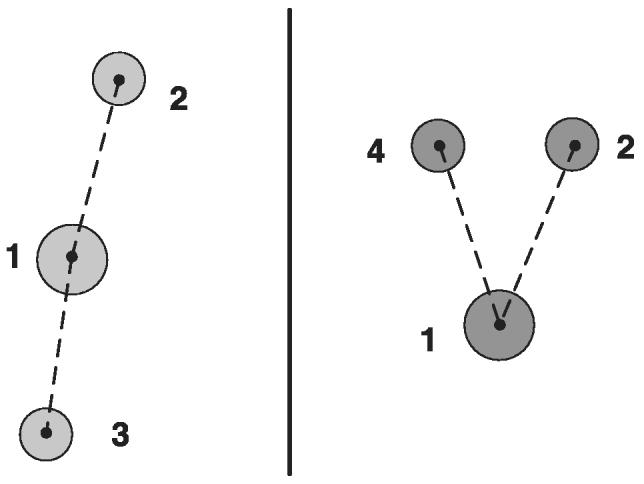
Illustration of the correspondence problem for two sets of features S_i and T_j with unequal number of features N^S = 3 (left) and N^T = 5 (right). Segments are shown as discs characterized by their index i, area $a_i^S$ and centroid location ${\overrightarrow{c}}_i^S$. Dashed lines represent the Euclidean distances between any two centroid locations.

The developed solution to the correspondence is presented here. Let us suppose that we extracted two sets of shape features S_a(a = 1, … , N^S) and T_b(b = 1, … , N^T) from two selected image frames $I_a^S$ and $I_b^T$ such as $S_i=\{{\overrightarrow{c}}_i^S,a_i^S\}$ and $T_j=\{{\overrightarrow{c}}_j^T,a_j^T\}$ , where ${\overrightarrow{c}}_k^{\Omega }$ are the 2D centroid locations and $a_k^{\Omega }$ are the area values. The number of features in each image is N^Ω, Ω = {S, T} and N^S does not necessarily equals N^T. An illustration of the correspondence problem is presented in Fig. 5 for N^S = 3 and N^S = 5.

In the first phase, the computation consists of (1) calculating a matrix of mutual distances $d_{\mathit{iu}}^S$ and $d_{\mathit{jv}}^T(i,u=1,\dots ,N^S\text{and}j,v=1,\dots ,N^T)$ for each set of segment centroids (e.g. dotted lines in Fig. 5), (2) finding a set of matching pairs of segments M_k and (3) sorting the matched segments based on the residuals of all matched centroids with respect to the estimated rigid transformation. To find a matching pair of segments, we first select a pair of segments S_i and T_j denoted by pivot segments, and introduce three similarity measures, such as (a) the area ratio A_ij(u, v), (b) the difference of Euclidian distances (residual) D_ij(u, v) and (c) the number of matching segments ${\mathcal{Q}}_{\mathit{ij}}$.

Pivoted by a pair of segments (S_i, T_j), we first compute the area ratio as ${\mathrm{A}}_{\mathit{ij}}(u,v)=\mid a_u^S∕a_v^T-1\mid$ for matching segments (S_u, T_v). Next, the difference of Euclidian distance is computed as ${\mathrm{D}}_{\mathit{ij}}(u,v)=\mid d_{\mathit{iu}}^S-d_{\mathit{jv}}^T\mid$. Finally, the number of matching pairs ${\mathcal{Q}}_{\mathit{ij}}$ is calculated by counting the number of pairs that satisfy both D_ij(u, v) < δ₁ and A_ij(u, v) < ε₁, where the value of δ₁ is the dissimilarity upper bound of a pair of distances, and ε₁ is the divergence upper bound of a ratio of two segment areas from 1. We not only maximize ${\mathcal{Q}}_{\mathit{ij}}$ but also remove the matches that do not satisfy the inequality ${\mathcal{Q}}_{\mathit{ij}}∕\left[\mathrm{Min}(N^S,N^T)\right]\ge {\lambda }_1$, where λ₁ ∈ [0, 1] is the lower bound of the normalized number of matches for a single pivot segment. Figure 6 shows the description of the defined similarity metrics.

Fig. 6.

Illustration of distance-based matching for two pivot segments $S_i=\{{\overrightarrow{c}}_i^S,a_i^S\}$ and $T_j=\{{\overrightarrow{c}}_j^T,a_j^T\}$. In order to find the best match, distance and area ratio of pairs of segments are compared to satisfy D_ij(u, v) < δ₁ and A_ij(u, v) < ε₁.

To find a final match M_k, we maximize a score function f(·) by incorporating three similarity metrics as follows:

$$M_k=\left\{(i,j)\mid (i,j)=\underset{i,j}{\arg \max }\left\{f\left({\mathcal{Q}}_{\mathit{ij}},\frac{1}{{\stackrel{-}{\mathrm{D}}}_{\mathit{ij}}},{\stackrel{-}{\mathrm{A}}}_{\mathit{ij}}\right)\right\}\right\}$$ (4)

where D̄_ij and Ā_ij are, respectively, the average error distance and area ratio pivoted by (S_i, T_j) for all matching pairs of (u, v), 0 ≤ k ≤ N^ST and N^ST is the number of matching pairs of segments (pivots). The function f(·) may be defined as an energy function or, more simply, a weighted product of all components. In our implementation, we used a weighted product of each component with normalization.

In the second phase, we first rotated segments from the set T_b(b = 1, … , N^T) to the coordinate system of the set S_a(a = 1, … , N^S) according to the parameters computed by selecting two best matches in the first phase. Next, vector-based matching is performed in a similar way as distance-based matching in the first phase. The major difference is in replacing the Euclidian distance metric D_ij(u, v) with the vector distance metric ${\mathrm{D}}_{\mathit{ij}}^{\ast }(u,v)$ defined in Eq. (5):

$${\mathrm{D}}_{\mathit{ij}}^{\ast }(u,v)=\Vert ({\overrightarrow{c}}_i^S-{\overrightarrow{c}}_u^S)-({\overrightarrow{c}}_j^T-{\overrightarrow{c}}_v^T)\Vert .$$ (5)

According to this distance metric, the vector distance incorporates both Euclidian distance and angular constrains about a pivot segment. Therefore, the matching performance is greatly increased compared with the first phase in terms of accuracy (mismatch) and the number of matching segments. The second phase contains the same three parameters as the first phase, and we denote them as ε₂, δ₂ and λ₂. In almost all experimental cases, we have set ε₁ = ε₂, δ₁ = δ₂ and λ₁ = λ₂ (see Table 3).

Table 3.

Manually selected parameters of the proposed 3D volume reconstruction method for the three evaluation pairs of images (T.S.: threshold of image S, T.T.: threshold of image T, M.R.: minimum region size for valid features, D.D.: disc diameter, ε: divergence of upper bound of ratio of two matching segment areas from 1, δ: dissimilarity upper bound of a pair of distances, λ: lower bound on the number of normalized matches).

Image	Phase	T.A (value)	T.B. (value)	M.R. (pixel)	D.D. (pixel)	ε (ratio)	δ (pixel)	λ (ratio)
1	1	1	1	50	2	1.2	20	0.4
	2	1	1	50	2	1.5	20	0.4
2	1	20	20	50	3	1.5	20	0.4
	2	20	20	50	3	1.5	20	0.4
3	1	20	20	50	3	1.5	15	0.4
	2	20	20	50	3	1.5	20	0.4

2.9. Image transformation and selection of feature pairs

As explained above, we carefully selected an affine transformation model for the final image transformation. Based on the material preparation procedure and the assumptions of the correspondence problem approach developed, the affine transformation model is constrained to only small amounts of scale and shear deformations.

Given the affine transformation model $\alpha :{\mathbb{R}}^2\to {\mathbb{R}}^2$, the image alignment can be performed by selecting at least three pairs of corresponding points and computing six affine transformation parameters as shown in Eq. (6). The values (x′, y′) = α(x, y) in Eq. (6) are the transformed coordinates of the original image coordinates (x, y) by affine transformation α(·). The four parameters a₀₀, a₁₀, a₀₁ and a₁₁ represent a 2 × 2 matrix compensating for scale, rotation and shear distortions in the final image. The two parameters t_x and t_y represent a 2D vector of translation:

$$\left[\begin{array}{c}\hfill x^{\prime }\hfill \\ \hfill y^{\prime }\hfill \end{array}\right]=\left[\begin{array}{cc}\hfill a_{00}\hfill & \hfill a_{01}\hfill \\ \hfill a_{10}\hfill & \hfill a_{11}\hfill \end{array}\right]\left[\begin{array}{c}\hfill x\hfill \\ \hfill y\hfill \end{array}\right]+\left[\begin{array}{c}\hfill t_x\hfill \\ \hfill t_y\hfill \end{array}\right].$$ (6)

From the viewpoint of image alignment accuracy, selected pairs of segment centroids should be well spatially distributed in each image and should not be collinear. If points are close to be collinear then the affine transformation parameters cannot be uniquely derived from a set of linear equations (more unknowns than the number of equations), which leads to large alignment errors. If points are locally clustered and do not cover an entire image spatially then the affine transformation is very accurate only in the proximity of the selected points. However, the affine transformation inaccuracy increases with distance from the selected points, which leads to large alignment errors because a registration error metric takes into account errors across the entire image area. In order to assess the pairs of matched centroid points in terms of their distribution and collinear arrangement, we have designed a compactness measure. It is defined as a ratio of the entire image area divided by the largest triangular area formed from the points. The measure is defined mathematically as

$$\mathit{Compactness}\mathit{Measure}=\frac{{\mathit{Area}}_{\mathit{IMACE}}}{{\mathit{Area}}_{\mathit{TRIANGLE}}}.$$ (7)

2.10. Optional transformation refinement

In this step, there is an option to accommodate a typical visual alignment by using the normalized correlation approach (Pratt, 1974). The morphology-based alignment performed so far could be refined based on intensity information in the same way as a human would incorporate morphology and intensity cues during alignment. This step is very computationally expensive with the computational complexity of O(image size × complexity of normalized correlation × M⁶), where M × M is the neighbourhood of a centroid point. One would select only a small spatial neighbourhood of the three centroid points to refine their locations based on the highest correlation value among all possible perturbations of centroid point locations. In practice, the size of the centroid point neighbourhood determines the importance assigned to morphology and intensity information during the alignment.

2.11. Image enhancement

The purpose of this step is to enhance CLSM image appearance for visual inspection. It is known that all fluorescent dyes bleach over time upon observation. This phenomenon, called photobleaching, occurs in confocal microscopy due to the high intensity of the laser illumination and the formation of oxygen radicals as a by-product of the photochemistry of fluorescence (reaction of oxygen radicals with the fluorescent dyes destroys the dyes). To remedy the photobleaching problem, one can use anti-fade agents (Franklin & Filion, 1985), such as N-propyl gallate, p-phenylenediamene (PPD), sodium azide, DABCO, or Citifluor, or apply image enhancement techniques such as contrast manipulation and histogram equalization (Stark & Fitzgerald, 1996).

Another approach to this problem is to restore or enhance image intensities. One of the most common techniques for image enhancement is histogram equalization (Benson et al., 1985). The histogram equalization method treats image intensities as random variables with values from the interval [0, 1] following a certain probability density function (PDF). By finding a transformation of the original PDF into a uniform PDF and applying it to image intensities, a newly formed image is characterized by lower contrast but uniform brightness.

Here, we chose to approach the problem with an image enhancement method that would be considered as a variation of histogram equalization (Gonzalez & Woods, 2002). The improved histogram equalization procedure involves two steps, (1) separating background pixels by thresholding with ω, and (2) applying the histogram equalization technique to foreground pixels. The final enhanced image values I_enhance are obtained according to:

$$\begin{array}{cc}\hfill & I_{\mathit{enhance}}=\mathit{HistogramEqualization}\left(I_{\mathit{fg}}\right);\hfill \\ \hfill & I_{\mathit{fg}}(x,y)=\{\begin{array}{cc}I(x,y):\hfill & \text{if}I(x,y)>\omega \hfill \\ \varphi :\hfill & \text{otherwise}\hfill \end{array}\phantom{\}}\hfill \end{array}$$ (8)

where I(x, y) and I_fg(x, y) are the original and foreground pixel value at (x, y), respectively, and ω is the threshold value. The symbol ϕ denotes background pixels, and the pixels labelled by ϕ are not considered during histogram equalization.

2.12. Evaluations of image alignment accuracy

Our primary evaluation criterion with regard to image alignment is its registration accuracy. We compare image alignment accuracy of the proposed fully automated method with registration accuracy achieved by human subjects using a manual registration method. There are three fundamental problems that arise during registration accuracy evaluations: (1) what to compare any registered image with, (2) how to compare multiple image alignment results and (3) how to evaluate accuracy of alignment (the choice of metrics).

Evaluation images

The challenge here lies in two partly conflicting objectives of our work. The first objective is to design a 3D volume reconstruction process that (a) aligns real data accurately and (b) is robust to many intensity and morphological deviations from a model. The second objective is to quantify the robustness and accuracy of the proposed 3D volume reconstruction process. If many sets of ground truth data were available then a 3D volume reconstruction process could be designed to compensate for known deviations leading to accurate and robust results (first objective). We could then easily quantify the accuracy and robustness of a 3D volume reconstruction process (second objective). However, if ground truth data are not available to meet the first objective, the design of a 3D volume reconstruction process has to be based on assumptions derived from theoretical considerations (fluorescence imaging and methodology of material preparation) and experimental observations (visual inspection of data and frame selection evaluations).

To meet the second objective, the need for evaluation (ground truth) data is even more pertinent and the problem of obtaining the data must be resolved. Given the frame selection procedure, the first and last frames within a subvolume are the best available type of registered data to assess accuracy and robustness, as illustrated in Fig. 7. Selection of evaluation images to be aligned is based on the following assumption. Presenting end frames of a real subvolume to humans is similar to showing the middle frames of two virtual subvolumes if morphological distortions due to preparation cut are neglected and an intensity profile is compromised. We model inter-subvolume morphological distortion δM^INTER = δM^INTRA + δM^PREP as a summation of intrasubvolume morphological variation δM^INTRA and the deformation introduced during material preparation δM^PREP. For evaluation purposes, we assume that the selected frames within a subvolume (known ‘ground truth’) approximate the case of selected frames from two spatially adjacent subvolumes (unknown ‘ground truth’). Thus, the experimental comparisons in this work are performed with the first and last frames within a subvolume, where the three selected pairs of frames shown in Fig. 8 came from those subvolumes that had the highest visual saliency scores of the first and last frames with a subvolume. This approach could be viewed as the most optimal compromise between the two conflicting objectives.

Fig. 7.

Real and virtual subvolumes of a specimen show two possible cuts of a specimen.

Fig. 8.

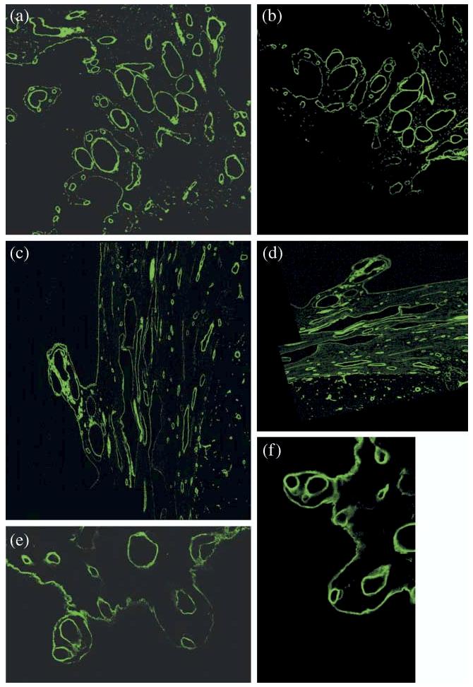
Illustration of the three selected pairs of evaluation images.

Figure 8 shows three pairs of misaligned images with known deformations by taking the first and last images along the z-axis within one CLSM stack (co-registered subvolume) and applying a representative affine transformation α^GT(·) to the last image with known transformation parameters. The representative affine transformation was determined from a set of all affine transformations obtained during manual 3D volume reconstructions. The last image before transformation is the ground truth image with respect to which both manual and automatic reconstructions are compared. All pixel coordinates of the transformed (ground truth) image ${\mathbf{P}}^{\mathit{GT}}=\{p_1^{\mathit{gt}},p_2^{\mathit{gt}},\dots ,p_n^{\mathit{gt}}\}$ are defined by the affine transformation ${\alpha }^{\mathit{GT}}:p_i\to p_i^{\mathit{gt}}$ for every pixel location P = {p₁, p₂, … , p_n}.

Registration software

The evaluation images are presented to a human subject or to an image alignment algorithm. For manual registration, the human–computer interface (HCI) for selecting points or segments is identical to our web-enabled HCI interface at http://i2k.ncsa.uiuc.edu/MedVolume. The manual and automated registration tools are part of the I2K software library.³

Evaluation metric

We chose to compare multiple alignment results by computing an average distance between a ground truth location and a location obtained from user-defined transformation (Lee & Bajcsy, 2005). The average distance E becomes our evaluation metric and is calculated over all image pixels according to:

$$E=\frac{1}{n}\sum _{i=1}^n\sqrt{{(p_{\mathit{ix}}^{\mathit{gt}}-p_{\mathit{ix}}^{\mathit{usr}})}^2+{(p_{\mathit{iy}}^{\mathit{gt}}-p_{\mathit{iy}}^{\mathit{usr}})}^2}$$ (9)

where n is the number of transformed image pixels, and ${\mathbf{P}}^{\mathit{USR}}=\{p_1^{\mathit{usr}},p_2^{\mathit{usr}},\dots ,p_n^{\mathit{usr}}\}$ are the transformed pixel coordinates according to the estimated affine transformation ${\alpha }^{\mathit{USR}}:p_i\to p_i^{\mathit{usr}}$ by user point selections. The set of affine parameters is obtained from manual (human subject's point selection and matching) or fully automated registration methods.

3. Results

3.1. Frame selection results

We evaluated two 3D volumes experimentally. One 3D volume was formed from four consecutive subvolumes consisting of 96 image frames (sample images are shown in Fig. 8), and a second was formed from six subvolumes consisting of 48 image frames. The entropy and contrast defined in Eqs (2) and (3) were multiplied according to Eq. (1), and the results are shown in Fig. 9 as a function of image frame index. These graphs demonstrate the combined entropy and contrast variations as a function of image frames from all subvolumes. The frame with maximum visual saliency score is selected automatically within each subvolume for alignment. For example, the frame indices 11 and 28 would be used for alignment of the first two depth-adjacent subvolumes because they correspond to the local maxima in Fig. 9 (left).

Fig. 9.

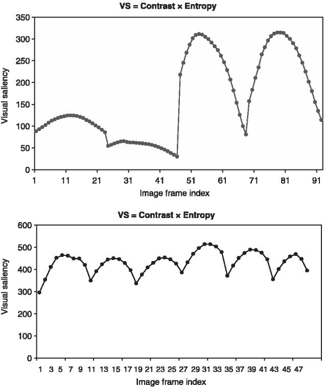
Evaluation of image frame selection from within each 3D subvolume to be used for alignment of the subvolumes. The graphs show combined visual saliency score as a function of image frame for two 3D volumes. The frame with maximum visual saliency score within each subvolume would be used for alignment.

Based on Fig. 9, one could always choose the middle frame of each physical section (subvolume) for image alignment and skip this processing step. From an accuracy viewpoint, this approach would lead to a suboptimal solution but with some computational savings. We discovered that the computational savings are negligible in comparison with all registration-related processing (less than a second per frame in comparison with several hours per frame for other processing steps according to Fig. 1). Experimental evaluations of the suboptimal accuracy loss led to the range of normalized correlation values in [0.59, 0.635] by computing the correlation of the middle frame (suboptimal solution) with all other 21 image frames inside one subvolume (potentially optimal solutions). Additional evaluations of normalized correlations for pairs of middle frames coming from adjacent cross-sections led to the range of values in [0.21, 0.27]. Thus, from our data, we concluded that based on the experimental data one would expect an inaccuracy due to a suboptimal solution to be between 0 (suboptimal and optimal solutions are identical) and 0.045/0.21 ≈ 21.43% (the worst case). Statistically, the distribution of the introduced inaccuracy would be skewed toward smaller values and would be data-dependent. In our experimental data shown in Fig. 9 (altogether ten subvolumes), 10% of the middle frames coincided with the optimal solution and the middle frame was displaced on average 2.5 frames from the optimal frame. In order to avoid these uncertainties, we recommend performing the frame selection step.

When we investigated tradeoffs between choosing the end frames of two spatially adjacent subvolumes (as opposed to selecting the frames closer to the middle frames within each subvolume), we discovered that although this method could be applied only after aligning subvolumes, it would still demonstrate the tradeoffs between intensity variations and morphological distortions along the z-axis (frame index), and hence guide us in an optimal frame selection. Figure 10 illustrates data that support the frame selection according to our proposed criteria rather than choosing the end frames.

Fig. 10.

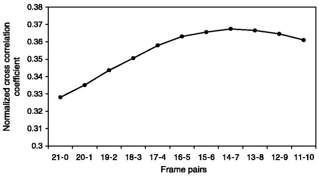
Evaluation of interframe similarity for two spatially adjacent subvolumes with 22 frames after alignment. The similarity is measured by normalized correlation (vertical axis). The horizontal axis refers to the pairs of frames that start with the end frames of subvolumes (21–0 ∼<Sub-Vol#1, frame#21> – <Sub-Vol#2, frame#0>) and finish with the middle frames (11–10 ∼<Sub-Vol#1, frame#11> – <Sub-Vol#2, frame#10>).

3.2. Manual alignment results

The experimental data consist of the total of 102 manual alignment trials with 20 human subjects. The compactness measure developed for automated alignment method (see Eq. 7) was applied to the set of points selected by human subjects, and the compactness measure values for all alignment trials are shown in Fig. 11. In order to eliminate the worst results, statistical analysis was applied. The elimination was based on a threshold value equal to 99.73% statistical confidence interval from the average and standard deviation values of all compactness measures (set to 1162.16). Figure 11 shows an alignment error as a function of the corresponding compactness measure reported for all experiments. Table 1 summarizes the results statistically per image pair.

Fig. 11.

Alignment error as a function of compactness measure associated with each trial. A high compactness measure implies that the control points selected during manual alignment are spatially dense or close to being collinear, thus leading to large alignment error. A hypothetical linear relationship of the variables is shown.

Table 1.

A summary of manual image alignment experiments for the 99.73% confidence interval. The table provides statistics computed from 86 human alignment trials after eliminating the worst six trials.

Error (pixels)	Manual (pixel-based)
Confidence interval = 9.73%
(compactness measure threshold = 1162.16)	Image 1	Image 2	Image 3	All Images
Average	43.57	22.42	21.49	29.22
SD	77.11	33.95	36.34	53.38

3.3. Automated alignment results

Table 2 details results obtained using automated alignment without and with the optional optimization step. The automated alignment leads to the same result every time the algorithm is executed with the same data, and therefore the standard deviation is equal to zero for each image pair and equal to 2.07 and 0.47 over all three image pairs without and with optimization, respectively. Some intermediate results for the automated alignment process are presented in Figs 12-15. After selecting the frames for alignment, the results of segmentation are shown in Fig. 12 (original) and Fig. 13 (segmentation) following the segmentation method described in Section 2.6. Figure 14 illustrates the correspondences found for the segments shown in Fig. 13 by considering centroid and area segment features (see Section 2.8). In Fig. 15, the circles denote three pairs of centroid points that were selected from the set of all pairs shown in Fig. 14 according to the proposed compactness measure defined in Eq. (7) and described in Section 2.9.

Table 2.

A summary of automatic image alignment experiments with and without optimization.

	Automatic with and without optimization
Error (pixels)	Image 1		Image 2		Image 3		Average
Optimization	no	yes	no	yes	no	yes	no	yes
Average	1.2839	1.4009	2.6508	2.1993	5.3500	2.2280	3.0949	1.9427
SD	0	0	0	0	0	0	2.0691	0.4694

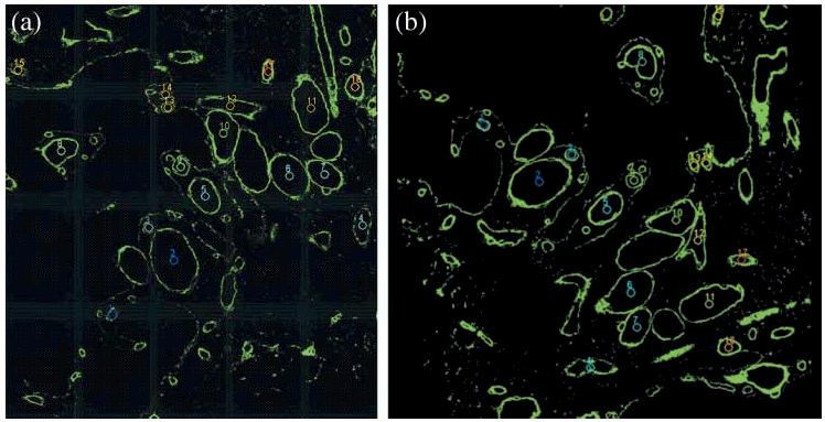
Fig. 12.

Two representative images that have to be aligned. The mathematical notations of these images in the text is $I_a^S\in V^S$ (left) and $I_b^T\in V^T$ (right). Human tonsil tissue stained for laminin.

Fig. 15.

The result of automated feature selection for the original images shown in Fig. 13 after they were processed to establish segment correspondences shown in Fig. 14. The different coloured circles represent three pairs of centroids selected automatically according to the compactness measure defined in Eq. (7).

Fig. 13.

Segmentation of input images shown in Fig. 12. Segmentation is performed by thresholding followed by connectivity analysis with a disc. The two images illustrate results obtained with different disc parameters [left image – T.S. (threshold S) = 10, right image – T.T. (threshold T) = 8, M.R. (minimum size of a region) = 80, and D.D. (disc diameter) = 1].

Fig. 14.

The correspondence outcome from two phases for the segments shown in Fig. 13. The left and right images are to be aligned. Overlays illustrate established correspondences between segments that are labelled from 1 to 17. The centroid locations of segments are sorted based on the correspondence error from the smallest to the largest.

The algorithmic parameters selected for the three evaluation pairs of images are shown in Table 3. The set of parameters includes (1) threshold values for images S and T, disc diameter and minimum acceptable segment size in the segmentation step, and (2) limiting values for centroid distances (ε₁, ε₂), segment areas (δ₁, δ₂) and numbers of segment matches (λ₁, λ₂) in the matching step. Ideally, one would like to perform general optimization of all parameters. In our case instead, the problem was constrained (1) to the same imaging device but acquiring data over a time period of several months, and (2) to the same class of specimens but prepared in separate batches. The parameters shown in Table 3 illustrate the small variability in the parameter values.

According to Table 2, the optimization step improved alignment accuracy for two out of the three test image pairs (test image pairs 2 and 3). The optimization step was conducted by choosing the correlation spatial neighbourhood size M = 5 to control (a) the amount of computation required and (b) the maximum range of shear and scale. In our experiments, all processing steps except for optimization took several seconds on a regular desktop computer. The optimization step on its own took on average 19.66 min (16, 21 and 22 min) on a single processor machine (3.0 GHz), for the three pairs of test images of pixel dimensions 578 × 549, 584 × 649 and 789 × 512. The offsets of the three centroids due to optimization were: (+1,+1), (0,0), (+1,0) for image 1; (−2,2), (1,2), (1,0) for image 2; and (2,−1), (2,2), (2,2) for image 3. The normalized correlation coefficient increased with optimization by 7.8, 21.3 and 12.4% for test image pairs 1, 2 and 3, respectively.

3.4. Image enhancement results

The techniques of histogram equalization (Fig. 16, middle) and improved histogram equalization (Fig. 16, right) were applied to images forming a 3D volume as described in Section 2.11. Based on a visual inspection of the two results in Fig. 16 (there are no metrics based on visual perception that are widely accepted in the literature), the overall intensity in the images is well adjusted with the original histogram equalization method; however, noisy pixels are overly highlighted and the edge intensity gradient is not preserved. By contrast, the proposed improved histogram equalization method provides better visual enhancement of fluorescent pixels while suppressing the image background.

Fig. 16.

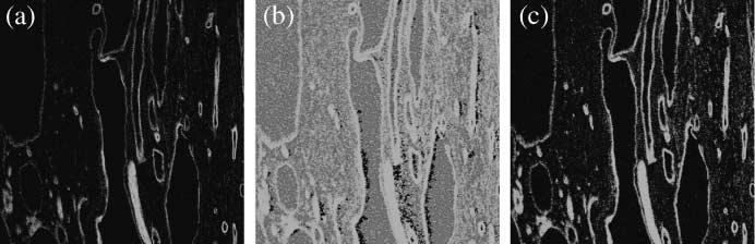
Comparison of two image enhancement techniques. Original CLSM image (left) and the results obtained by histogram equalization (middle), and by the proposed improved histogram equalization method (right) with background subtraction (threshold valuw ω = 20).

4. Discussion

The design of a 3D volume reconstruction process drew from theoretical considerations (fluorescence imaging and material preparation methodology) and experimental observations (visual inspection of data and frame selection evaluations). Frame selection experiments were shown to illustrate the tradeoffs between morphological distortion and intensity variations. The results obtained during frame selection provided additional insight into many of the registration decisions, e.g. transformation model selection, and morphological and intensity invariance.

For the evaluation of image alignment, the underlying assumptions are that: (a) the three evaluation images prepared (first and last frames within a stack) are realistic representatives of slide-to-slide alignment cases, where two cross-sections might have (i) missing, (ii) new or (iii) warped structures with a priori unknown intensity variations; (b) HCI of our software registration tools are user-friendly; (c) 102 manual alignment trials with 20 human subjects form a statistically significant pool of measurement samples; and (d) the global evaluation metric to Eq. (9) is appropriate for comparing multiple alignment results. Observations of a material preparation procedure led us to the use of the affine transformation model as modelled by the evaluation images. To obtain better understanding of rigid vs. affine transformation models, we implemented a web-enabled simulation tool at http://i2k.ncsa.uiuc.edu/MedVolume. Under the above assumptions and based on the image alignment results obtained, we concluded that manual (pixel-based) image alignment is less accurate and less consistent (large standard deviation) than the fully automated alignment (on average, 9.4 or 15 times larger alignment error without or with optimization, respectively, and 25.8 or 113.7 times larger standard deviation without or with optimization, respectively, in the 99.73% confidence interval).

The limitations of the fully automated 3D reconstruction system resulted from those inherent to all modelling assumptions, such as (a) the presence of partially closed contours of fluorescent pixels, (b) shape invariance along the z-axis for two depth-adjacent subvolumes, (c) satisfactory SNR, (d) limited amount of scale and shear deformations due to specimen preparation and imaging, and (e) a sufficient number of features detected (at least three pairs). In addition, selection and optimization of algorithmic parameters still pose challenges for automation, although the algorithmic parameters in Table 3 demonstrated a very negligible change from image to image. The limitations of the manual 3D volume reconstruction are clearly consistency, the cost of human time needed to perform image alignment and knowledge requirements to achieve good alignment accuracy (e.g. the time for training human subjects). In general, the time spent on each 3D volume reconstruction task is non-linearly proportional to the resulting quality, with certain insurmountable quality limits.

As indicated in Section 2.10, the inclusion of the alignment optimization step is optional and depends on input data. One would expect to obtain higher alignment accuracy with optimization than without optimization. The optimization step is based on pixel-to-pixel intensity correlation that should compensate for inaccuracies introduced by centroid point extraction (segmentation inaccuracy) and segment representation (shape characteristics limited to centroid and segment size), assuming correct pairs of segments were established. However, we observed that for larger size segments these inaccuracies are larger than for smaller size segments. For example, the average segment size of the three pairs of segments selected for computing the registration transformation parameters was 177, 222 and 1498 pixels for test image pairs 1, 2 and 3, respectively. Thus, we hypothesize that the optimization step will not improve alignment accuracy (and should not be used) if the set of matched segments consists of small-sized segments (e.g. less than 200 pixels but larger than the algorithmically defined minimum size threshold equal to 50 pixels). This rule for inclusion of the optimization step could be explained by the presence of larger shape variations for larger sized segments that were not captured by the two descriptors (centroid and size) and brought larger mismatch of lit up pixels defining segment boundaries. Intensity-based optimization therefore leads to alignment improvement. By contrast, smaller sized segments are represented sufficiently accurately with the set of segmented pixels and the two shape descriptors, and any additional optimization based on intensity information might worsen the results due to intensity noise. Finally, the computational cost of optimization should be offset by the alignment accuracy gain. In our experiments, an average of 19.66 min per optimization would not be considered as unreasonable. However, significantly larger execution time could be expected for larger images because the computational cost of optimization will increase exponentially with image size, and a tradeoff study of feasibility vs. accuracy gain for such experiments should be conducted beforehand.

5. Conclusions

We have presented a solution to 3D volume reconstruction of blood vessels and vasculogenic mimicry patterns in histological sections of uveal melanoma from serial fluorescently labelled paraffin sections labelled with antibodies to CD34 and laminin and studied by CLSM. Under the assumptions discussed above and including evaluation data, registration software, a number of trials and evaluation metrics, our work demonstrates significant benefits of automation for 3D volume reconstruction in terms of accuracy achieved (on average, 9.4 or 15 times smaller alignment error without or with optimization, respectively) and consistency (25.8 or 113.7 times smaller standard deviation without or with optimization, respectively) of the results and performance time. We have also outlined the limitations of fully automated and manual 3D volume reconstruction systems, and described related automation challenges. We have tried to show that given computational resources and repetitive experimental data, the automated alignment provides more accurate and consistent results than a manual alignment approach. With the proposed approach, the automation will reduce alignment execution time and future costs, as the price of more powerful computers decreases.

To our knowledge, there have been developed no robust and accurate fully automated 3D volume reconstruction methods from a stack of CLSM images without artificially inserted fiduciary markers. Our research work is also unique in terms of forming a complete system for medical inspection of 3D volumes reconstructed from CLSM images. Our approach to automating the reconstruction process incorporates the tradeoffs between computational requirements and uncertainty of the resulting reconstructions introduced by each processing step. For example, just to perform alignment refinement over a small pixel neighbourhood requires significant computational resources (Kooper et al., 2005). Thus, the approach based on morphology-based alignment followed by intensity-based refinement accommodates our prior knowledge regarding the data and limitations of our computational resources. This paper contributes to the presentation and development of a 3D volume reconstruction process with automated methods for (a) frame selection from a pair of depth-adjacent subvolumes, (b) image alignment and (c) visual enhancement. Our 3D volume reconstruction process is supported by (1) conducting experiments to compare (a) optimal and suboptimal frame selection, and (b) manual and fully automated alignment procedures, and (2) explaining the reasons behind choosing (a) the affine transformation model as opposed to a rigid model, and (b) morphology-based alignment followed by intensity-based refinement.

References

- Alkemper J, Voorhees PW. Quantitative serial sectioning analysis. J. Microsc. 2001;201:388–394. doi: 10.1046/j.1365-2818.2001.00832.x. [DOI] [PubMed] [Google Scholar]
- Benson D, Bryan J, Plant A, Gotto A, Smith L. Digital imaging fluorescence microscopy: spatial heterogeneity of photobleaching rate constants in individual cells. J. Cell Biol. 1985;100:1309–1323. doi: 10.1083/jcb.100.4.1309. [DOI] [PMC free article] [PubMed] [Google Scholar]
- Brown L. A survey of image registration techniques. ACM Comp. Surveys. 1992;24:326–276. [Google Scholar]
- Dorst L. First order error propagation of the procrustes method for 3D attitude estimation. IEEE Trans. Pattern Anal. Mach. Intell. 2005;27:221–229. doi: 10.1109/TPAMI.2005.29. [DOI] [PubMed] [Google Scholar]
- Duda R, Hart P, Stork D. Pattern Classification. 2nd edn. Wiley-Interscience; New York: 2001. [Google Scholar]
- Folberg R, Maniotis AJ. Vasculogenic mimicry. APMIS. 2004;112:508–525. doi: 10.1111/j.1600-0463.2004.apm11207-0810.x. [DOI] [PubMed] [Google Scholar]
- Franklin A, Filion W. A new technique for retarding fading of fluorescence: DPX-BME. Stain Technol. 1985;60:125–153. doi: 10.3109/10520298509113903. [DOI] [PubMed] [Google Scholar]
- Gonzalez RC, Woods RE. Digital Image Processing. 2nd edn. Prentice Hall Inc; New Jersey: 2002. [Google Scholar]
- Hill D, Batchelor P, Holden M, Hawkes D. Medical image registration. Phys. Med. Biol. 2001;46:R1–R45. doi: 10.1088/0031-9155/46/3/201. [DOI] [PubMed] [Google Scholar]
- Kooper R, Shirk A, Lee S-C, Lin A, Folberg R, Bajcsy P. 3D volume reconstruction using web services. Proc. IEEE Int. Conf. Web Services. 2005;2:709–716. doi: 10.1016/j.compbiomed.2008.01.015. [DOI] [PMC free article] [PubMed] [Google Scholar]
- Lee S-C, Bajcsy P. Feature based registration of fluorescent LSCM imagery using region centroids. Proc. SPIE. 2005;5747:170–181. [Google Scholar]
- Maintz JBA, Viergever MA. A survey of medical image registration. Med. Image Anal. 1998;2:1–36. doi: 10.1016/s1361-8415(01)80026-8. [DOI] [PubMed] [Google Scholar]
- Maniotis A, Chen X, Garcia C, DeChristopher P, Wu D, Pe'er J, Folberg R. Control of melanoma morphogenesis, endothelial survival, and perfusion by extracellular matrix. Lab. Invest. 2002;82:1031–1043. doi: 10.1097/01.lab.0000024362.12721.67. [DOI] [PubMed] [Google Scholar]
- Nocito A, Kononen J, Kallioniemi OP, Sauter G. Tissue microarrays (TMAs) for high-throughput molecular pathology research. Int. J. Cancer. 2001;94:1–5. doi: 10.1002/ijc.1385. [DOI] [PubMed] [Google Scholar]
- Papadimitriou C, Yapijakis C, Davaki P. Use of truncated pyramid representation methodology in three-dimensional reconstruction: an example. J. Microsc. 2004;214:70–75. doi: 10.1111/j.0022-2720.2004.01298.x. [DOI] [PubMed] [Google Scholar]
- Pratt WK. Correlation techniques for image registration. IEEE Trans. Aerospace Eng. Sys. 1974;10:353–358. [Google Scholar]
- Russ JC. The Image Processing Handbook. 3rd edn. CRC Press; Boca Raton: 1999. [Google Scholar]
- Spacek J. Three-dimensional reconstruction of astroglia and oligodendroglia cells. Z. Zellforsch. Mikroskop. Anat. 1971;112:430–442. [PubMed] [Google Scholar]
- Stark JA, Fitzgerald WJ. An alternative algorithm for adaptive histogram equalization. Comput. Vis. Graph. Image Process. 1996;56:180–185. [Google Scholar]
- Wu J, Rajwa B, Filmer DL, Hoffmann CM, Yuan B, Chiang C, Sturgis J, Robinson JP. Automated quantification and reconstruction of collagen matrix from 3D confocal datasets. J. Microsc. 2003;210:158–165. doi: 10.1046/j.1365-2818.2003.01191.x. [DOI] [PubMed] [Google Scholar]
- Zitova B, Flusser J. Image registration methods: a survey. Image Vis. Comp. 2003;21:977–1000. [Google Scholar]