Deterministic and Stochastic Regimes of Asexual Evolution on Rugged Fitness Landscapes

Abstract

We study the adaptation dynamics of an initially maladapted asexual population with genotypes represented by binary sequences of length L. The population evolves in a maximally rugged fitness landscape with a large number of local optima. We find that whether the evolutionary trajectory is deterministic or stochastic depends on the effective mutational distance d_eff up to which the population can spread in genotype space. For d_eff = L, the deterministic quasi-species theory operates while for d_eff < 1, the evolution is completely stochastic. Between these two limiting cases, the dynamics are described by a local quasi-species theory below a crossover time T_× while above T_× the population gets trapped at a local fitness peak and manages to find a better peak via either stochastic tunneling or double mutations. In the stochastic regime d_eff < 1, we identify two subregimes associated with clonal interference and uphill adaptive walks, respectively. We argue that our findings are relevant to the interpretation of evolution experiments with microbial populations.

THE question of whether the course of evolution is predetermined—and if yes, to what extent and under what conditions this might be so—has recently attracted the attention of many researchers (Wahl and Krakauer 2000; Rouzine et al. 2001; Yedid and Bell 2002). The answer to this question, particularly for large populations, is not obvious since the trajectories traced out during evolution are shaped by the interplay of the (deterministic) selective forces encoded in the fitness landscape and the stochasticity of the mutational process, which limits the ability of the population to find and maintain favorable genotypes.

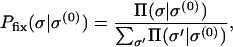
We address this question for an asexual population of size N and binary genotype sequences of length L evolving on a fitness landscape. As there is considerable evidence (Whitlock et al. 1995) for interactions among gene loci (or epistasis), it is important to consider the evolutionary process on a landscape that includes them. Such interactions may (Wright 1932; Gavrilets 2004; Weinreich et al. 2005) or may not (Lunzer et al. 2005; Weinreich et al. 2006) give rise to multiple peaks in the fitness landscape (Jain and Krug 2007). But at least on a qualitative level, recent experiments on microbial populations (Elena and Lenski 2003) support the notion that the fitness landscape underlying the adaptive process has multiple peaks (Korona et al. 1994; Lenski and Travisano 1994; Burch and Chao 1999, 2000; Elena and Sanjuan 2003). Motivated by this, we consider the dynamics of the evolutionary process on maximally rugged landscapes (Kauffman and Levin 1987; Flyvbjerg and Lautrup 1992) that have high epistasis and a large number of adaptive peaks separated by valleys.

A detailed theoretical description of the evolution of a population subject to the combined effects of selection, mutation, and stochastic drift in a complex fitness landscape constitutes a formidable problem, and previous studies have usually considered two limiting cases on the basis of the size N of the population and the mutation probability μ per generation per base (or gene locus). When the total number of mutants produced in a generation, NLμ, is small, the population consists of a single genotype at most times. Occasionally a mutation occurs in a single individual, which may become fixed in the population with a probability depending on the fitness advantage of the mutant. The population thus performs an adaptive walk along a set of genotypes connected by single point mutations, which is biased toward high fitnesses and terminates at a local fitness maximum (Gillespie 1984; Kauffman and Levin 1987; Macken and Perelson 1989; Macken et al. 1991; Flyvbjerg and Lautrup 1992; Orr 2002). Clearly, the trajectory traced out by the population in this case is determined stochastically. In the other extreme limit of applicable to enormously large populations, each (relevant) genotype is populated by many individuals and the stochasticity inherent in the selection of individuals for reproduction can be neglected. This is the regime of deterministic mutation–selection dynamics described by the quasi-species model, which was originally introduced in the context of prebiotic molecular evolution (Eigen 1971; Eigen et al. 1989; Baake and Gabriel 2000; Jain and Krug 2007).

Thus, in these two extreme cases the population either has many weighted paths available or follows a single predetermined route to the global peak. One would like to know: What is the nature of the dynamics for parameters lying between these two limits? In models, we describe the model and introduce a parameter d_eff on the basis of which various dynamical regimes are distinguished. The effective distance d_eff is basically a measure of the extent to which a finite population can spread in the space of genotype sequences by mutations. For infinite populations, this distance equals the diameter L of the entire sequence space, and we discuss this case in quasi-species dynamics. We start with our earlier work on quasi-species evolution (Krug and Karl 2003; Jain and Krug 2005), which provides in a suitably defined strong selection limit a very transparent picture of the evolutionary trajectories and the genotypes that are encountered by a population moving toward the global fitness peak. We show that provided the mutation probability μ is sufficiently small, the analysis of Jain and Krug (2005) holds beyond the strong selection limit and the evolutionary trajectories obtained at different values of μ can be superimposed by a simple rescaling of time. finite populations deals with the two subcases 1 ≤ d_eff < L and d_eff < 1. The basic idea in the first case is that the finite population behaves like a quasi-species in an effective sequence space up to a certain timescale above which the stochastic evolution takes over. We estimate the time at which the crossover from deterministic to stochastic evolution occurs. For d_eff < 1, the dynamics are stochastic at all times but depending on the product NLμ, the dynamics may be characterized by the “clonal interference” of several genotypes (Gerrish and Lenski 1998) or they may follow the adaptive walk scenario described above. In each case, we describe several individual fitness trajectories in detail both as a function of time and as a function of the system parameters. Finally, in the last section we summarize our results and discuss the relation of this work with that of others.

MODELS

We consider a haploid, asexual population with genotypes drawn from the space of binary sequences σ = {σ₁, …, σ_L} of length L, where σ_i = 0 or 1. Depending on the context, a genotype can be thought to represent a small genome, a single gene, or a sequence of L biallelic genetic loci. A fitness W(σ) ≥ 0 proportional to the expected number of offspring produced by an individual of genotype σ is associated with each sequence. Reproduction occurs in discrete, nonoverlapping generations. The structure of the population is monitored through the frequency X(σ, t) of individuals of genotype σ in generation t.

To simulate the stochastic evolution, a population of fixed size N is propagated via standard Wright–Fisher sampling; i.e., each individual in the new population chooses an ancestor from the old population with a probability proportional to the fitness of the ancestor. Subsequently, point mutations are introduced with probability μ per locus per generation. In the limit of very large populations, this leads to a deterministic time evolution for the average frequency , where the angular brackets refer to an average over all realizations of the sampling process. The evolution equation reads as

(1)

(Jain and Krug 2007), where

(2)

is the probability of producing σ as a mutant of σ′ in one generation, and d(σ, σ′) denotes the Hamming distance between the two genotypes (i.e., the number of single point mutations in which they differ). Instead of simulating a large (infinite) population, we numerically iterate the above discrete-time equation. For future reference we note that the nonlinear evolution (1) is equivalent to the linear iteration

(3)

for the unnormalized frequency , where (Jain and Krug 2007).

To generate a maximally rugged fitness landscape, the fitness values W(σ) are chosen independently from a common exponential distribution P(W) = e^−W with unit mean. In the language of Kauffman's rugged landscape models in which the fitness contribution of each of the L loci depends randomly on K other loci, our uncorrelated landscape corresponds to K = L − 1 and hence the limit of strong epistasis (Kauffman 1993). In particular, sign epistasis, in the sense that a particular point mutation may be beneficial or deleterious depending on the genetic background (Weinreich et al. 2005), is common in these landscapes. We also note that the selection coefficient for a mutant of genotype σ in a background of genotype σ′ is given by

(4)

and the probability to find a genotype of fitness larger than W is

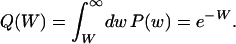(5)

We recall some typical properties of maximally rugged landscapes (Kauffman and Levin 1987; Kauffman 1993), which follow from elementary order statistics. For S exponentially distributed random variables, the average value of the maximum is given by ln S (David 1970; Sornette 2000), which yields the expected fitness 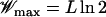of the globally fittest among the 2^L genotypes. Correspondingly, the typical fitness of a local maximum that is a genotype without fitter one-mutant neighbors is . Since the probability that a genotype is a local maximum is 1/(L + 1), there are on an average 2^L/(L + 1) local maxima in these landscapes. For such a genotype σ with fitness surrounded by typical genotypes of fitness , the selection coefficient 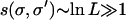. In this sense, we are dealing with a situation of strong selection throughout this article.

For the purposes of illustration, we base much of the discussion below on two reference landscapes, each of which is a single realization of landscapes with sequence length L = 15 and 6. The starting sequence σ⁽⁰⁾ is a randomly chosen genotype at which the population finds itself in the beginning of the adaptation process. For our reference landscapes, σ⁽⁰⁾ is of relatively poor fitness with value W(σ⁽⁰⁾) ≈ 0.13 for both cases. This has a rank 28,795 among 2¹⁵ = 32,768 genotypes and 55 among 2⁶ = 64 genotypes where the global maximum is assigned the rank 0. The global peak is located at Hamming distance 10 and 2 from σ⁽⁰⁾ with fitness W_max = 10.72 and 4.29 for L = 15 and L = 6, respectively. In the following discussion, instead of specifying actual fitness values for each sequence, we provide their ranks as a subscript in the population density X_rank(σ, t).

In the subsequent sections, we distinguish the dynamics on the basis of a parameter d_eff, which is a measure of the typical extension of the population in genotype space, and for strong selection, it is given by

(6)

Due to the quasi-species Equation 1, the average number of individuals produced in one generation at a sequence σ located at distance d(σ, σ⁽⁰⁾) from a localized population of size N is given by . Thus the maximum distance d_eff at which at least one individual (required for asexual reproduction) can be detected after one generation is given by (6). However, in the next generation, the mutants of σ⁽⁰⁾ can acquire further mutations thus extending the spread of the population beyond d_eff. We argue below that for landscapes with large selection coefficients as is the case with our rugged landscapes, the above definition is nevertheless a good approximation.

To see this, let us consider the evolution in a landscape with infinite selection coefficients for which (6) is exact. As argued above, starting from a localized population at σ⁽⁰⁾, at t = 1 the population spreads over a typical distance d_eff. If the landscape is such that all the sequences except the best one among the ones available within d_eff are lethal (i.e., with fitness zero), then in the next generation the population will move to the lone viable genotype (fitter than σ⁽⁰⁾). This sequence in turn can be treated as the new σ⁽⁰⁾ and the above argument can be applied recursively.

That (6) cannot hold for weak selection can be seen by considering the flat fitness landscape (with selection coefficients zero) for which it is known that the average Hamming distance over which the population spreads is

(7)

(Derrida and Peliti 1991) and which for large Nμ is simply L/2. Away from these two limiting cases, one may expect an explicit dependence on the relevant selection coefficients. For rugged landscapes, one can get an idea of such a dependence at late times when (as explained in finite populations) the population gets trapped at a sequence whose mutants within d_eff are not fitter than itself. In such a case, the population at the peak and its surrounding valley reaches a stationary state and forms a quasi-species. Approximating the surrounding genotypes by a flat fitness landscape with W(σ′) = 1 and the localizing sequence with fitness , an analysis within the unidirectional approximation shows that the population distribution is an exponential

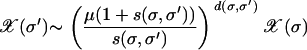(8)

(Higgs 1994). Defining d_eff as the genetic distance at which the population fraction falls to 1/N, the resulting expression for d_eff is given by

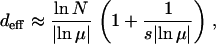(9)

which reduces to (6) with a correction that becomes negligible for 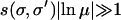. When either the selection is weak or the mutation rate is large, the effective mutational distance is larger than given by (6). In the following sections, we study three distinct cases classified on the basis of distance (6): (a) d_eff = L, (b) 1 ≤ d_eff < L, and (c) d_eff < 1.

QUASI-SPECIES DYNAMICS

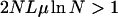
When the population , the effective distance d_eff = L and the population can spread all over the Hamming space. For small mutation probability μ (of the order 10⁻³–10⁻⁸) that we consider here, this population size far exceeds the number of available genotypes. The requirement of such a large population size for a completely deterministic description comes from (2), according to which the mutation probability decreases exponentially with the distance.

The discrete-time quasi-species Equation 1 was iterated numerically for the population fraction , where we have labeled a sequence by its rank and Hamming distance from σ⁽⁰⁾. The time evolution is depicted in Figure 1 for various μ and fixed L. Since 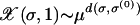, all the mutants become available immediately with a concentration decreasing exponentially with the distance from the parent sequence. As a result, the population at fitter sequences closer to the parent increases and that at σ⁽⁰⁾ decreases. One of these fit sequences becomes dominant in the sense that it supports the largest population. This sequence is in turn overtaken by a fitter sequence close to it, and this process of leadership changes goes on until the population has reached the global maximum. We are interested in the evolutionary trajectory traced out by the most populated sequence σ*(t) at time t.

Figure 1.—

Quasi-species evolution of the populations . The numerical iteration of Equation 1 is shown for μ = 10⁻⁸, 10⁻⁶, and 10⁻⁴ (top to bottom) with L = 15, starting from all the populations at sequence σ⁽⁰⁾ in the fitness landscape explained in the text. The sequences with fraction ≥0.005 are shown.

The analysis of Krug and Karl (2003) and Jain and Krug (2005) provides a simple way of identifying the genotype σ* for a given landscape and a given starting sequence. It is based on a particular strong selection limit, in which the mutation rate is scaled to zero and the fitnesses are scaled to infinity in such a way that the (appropriately normalized) logarithmic population fractions remain well behaved. The key observation is that the behavior of the evolutionary trajectory σ*(t) can be accurately predicted by simply assuming that the mutations can be turned off once the sequence space has been “seeded” by the population fraction ∼μ^d that is established by mutations after the first generation. Thus, each unnormalized population frequency changes exponentially in time according to its own fitness, from an initial value proportional to . In logarithmic variables, this implies the simple linear time evolution

(10)

(see also Zhang 1997). Since the first term on the right-hand side is the same for all sequences in a shell of constant Hamming distance d(σ, σ⁽⁰⁾), within each shell only the sequence with the largest fitness needs to be considered for determining σ*(t). It is also evident from (10) that among these shell fitnesses only fitness records, that is, sequences whose fitness is larger than the fitnesses in all shells closer to σ⁽⁰⁾, can possibly partake in the evolutionary trajectory. Fitness records can be identified purely on the basis of the fitness rank. Their statistical properties are independent of the underlying fitness distribution, but depend on the geometry of the sequence space (Jain and Krug 2005; Krug and Jain 2005).

The set of sequences {σ*} making up the evolutionary trajectory is a subset of the fitness records, from which those records are eliminated that are being bypassed by a fitter but more distant record before reaching the status of the most populated genotype (Krug and Karl 2003; Sire et al. 2006). To decide whether a given record is bypassed, the actual fitness values and not just their ranks are needed. Bypassing is a significant effect: it reduces the number of steps in the evolutionary trajectory from the number of records, which is of order L, to the order for logarithmic fitness distributions of the exponential type (Jain and Krug 2005; Krug and Jain 2005). Thus, not all of the L + 1 mutant classes can appear in the trajectory and in fact, only a vanishing fraction of a total of 2^L genotypes actually appear (Figure 1).

When applied to our reference landscape, the above analysis predicts an evolutionary trajectory involving the genotypes with ranks 28,795, 4688, 5, 1, and 0 in shells 0, 1, 2, 7, and 10, respectively, which are precisely the ones that appear in Figure 1. Each of these genotypes is also a record, none of which is bypassed in the landscape used here. To see bypassing of the contending genotypes, we need to consider larger L as the number of bypassed sequences increases with L.

As Figure 1 shows, although the set {σ*} remains the same for a broad range of mutation probability μ, the timing of the appearance of new mutants and the polymorphism of the population depends on μ. These effects are also reflected in the stepwise behavior of the population averaged fitness 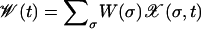in Figure 2. For smaller μ, adaptive events occur at later times. This is expected on the basis of (10) from which μ can be eliminated by a rescaling of time with |ln μ|. Indeed, the inset shows that the timing of the peak shifts can be made to coincide by scaling time with |ln μ|. The other effect with increasing μ is that the transitions between fitness peaks become more gradual (Krug and Halpin-Healy 1993), and the fitness level at a given (rescaled) time is lowered. This happens due to an increase in the diversity (the number of genotypes present in the population) that is controlled by the probability 1 − (1 − μ)^L ≈ μL for any mutation to occur. For the largest mutation probability μ = 10⁻² that we consider here, this probability is significant and the mutational load (Haldane 1927) can be estimated as follows. Using the quasi-species Equation 1 in the steady state within unidirectional approximation (Jain and Krug 2007) for the master sequence with fitness W(σ*), it immediately follows that the population fitness is given by W(σ*)e^−μL for large L and small μ. The mutational load is thus W(σ*)(1 − e^−μL) and the fitness is reduced by a factor e^−μL ≈ 0.86 for μ = 0.01 and L = 15, in very good agreement with the data in Figure 2. To summarize, the mutations affect the dynamics in two respects: on decreasing μ, the new mutants get fitter but are slower to appear (“slow-but-fit”).

Figure 2.—

Punctuated rise of the average fitness for fixed landscape and fixed initial condition in the quasi-species model with genome length L = 15. The solid line is the fitness W_max of the global maximum and the dashed line is e^−μLW_max with μ = 10⁻². The steps become more diffuse as μ increases, and the fitness level is reduced for the largest value of μ due to the broadening of the genotype distribution. Inset: average fitness plotted as a function of t/|ln μ| to show the scaling of jump times.

FINITE POPULATIONS

As we discussed above, in the infinite population limit all the genotypes are immediately occupied so that the subsequent dynamics involving the fit genotypes can be approximated as largely due to the selection process. For finite N on the other hand, the population distribution has a finite support d_eff at any time. Then if the distance to the genotype that offers selective advantage over the currently dominant one is larger than d_eff, or the distance d_eff is less than unity, the average number of individuals at the desired distance is smaller than one. One cannot work with averages under such circumstances and must take fluctuations arising due to rare mutations into account.

Crossover from deterministic to stochastic dynamics:

We first consider the case when 1 ≤ d_eff < L. Starting from a parent sequence σ⁽⁰⁾ supporting a population , the mutants can spread up to a shell at a distance d_eff < L. Then provided the selection coefficient involving the fittest and the next few fittest sequences within d_eff is large, the dynamics within this distance are similar to the quasi-species case in that the population at the fittest sequence in each shell competes with the one in other occupied shells and passing through sequences at which it becomes dominant in the least time finds the best available sequence σ* within d_eff of σ⁽⁰⁾. The last step is akin to finding the global maximum in the quasi-species case. If, however, the selection is not strong, several fit genotypes get populated, and due to a mutation in this set of fit sequences, the population may be able to find a sequence even fitter than the fittest sequence σ* within d_eff. In such an event, the fittest sequence within d_eff still achieves a majority status but only momentarily. A similar process is repeated within shells at radius d_eff from the new most populated sequence σ*. The above deterministic process is expected to occur for individual trajectories obtained in stochastic simulations as long as the population can find a sequence better than the current σ* within a distance d_eff. In particular, for d_eff ∼ 1, the local quasi-species evolution continues until the population hits a local peak, after which stochastic evolution takes over. The latter typically involves “crossing the valley” via less fit nearest-neighbor mutants to a better peak than the current one.

In Figure 3, we chose d_eff slightly above unity; since at any time typically the population can sense only L sequences, we work with a small sequence space of length L = 6 to reduce the number 2^L − L of unoccupied sequences. Also, we keep the mutation probability μ somewhat large since for d_eff close to one, N ∼ μ⁻¹ and Wright–Fisher sampling requires operations of order N per time step. Note that in this case the number of genotypes 2^L = 64 is much smaller than the population size. Nevertheless, we will see that the dynamics is far from the deterministic quasi-species limit, because the more stringent condition d_eff = L is not met. Since doubling d_eff requires increasing the population size from N to N², it is clear that fully deterministic behavior can be realized only under extreme conditions.

Figure 3.—

Evolutionary trajectories in a sequence space of length L = 6 with N = 2¹⁴, μ = 10⁻⁴ so that Nμ ≈ 1.64 and d_eff ≈ 1.05. The population fraction is denoted by X_rank(σ), where the σ_i's that do not change in the course of time are represented by a dash. Only the sequences with population fraction ≥0.05 are shown. In the initial phase, the three populations X₅₅, X₂₈, and X₅ occur in all of the above trajectories and have rather similar curves, supporting deterministic evolution. At later times, the population escapes the local peak with rank 5 via tunneling (top) and by a double mutation (center).

Deterministic dynamics:

The different runs in Figure 3 correspond to different sampling noise with all the other parameters kept the same. We start with all the individuals at sequence σ⁽⁰⁾ with rank 55. Since d_eff is close to one, the population spreads from here to sequences within Hamming distance unity of σ⁽⁰⁾ and moves to the best sequence among them, namely the sequence with rank 28. In this case, there is no bypassing (discussed in quasi-species dynamics) of a fit sequence and the best sequence in the first shell becomes the most populated sequence σ*. As the population at this sequence grows, the chance that it will produce its one-mutant neighbors also increases; in fact, a mutant better than σ* appears at time τ ∼ (1/s)ln(s/Nμ²), where the selection coefficient ), when the fraction at the current σ* becomes ∼1/Nμ (Wahl and Krakauer 2000). The population then starts growing at the sequence with rank 5, which is the best sequence in the first shell centered about the sequence ranked 28. The process so far is deterministic as is evident from the three runs. Note that the set σ* obtained using the local quasi-species theory will in general be different from the quasi-species analysis of the Hamming space containing all shells up to the shell in which the local peak is situated; this is because the sequences obtained in the former case can be outcompeted by fitter mutants before reaching fixation as discussed in the last section. For instance, if we apply the deterministic prescription to the Hamming space restricted to shell 2 about σ⁽⁰⁾, the sequence ranked 5 will not appear in the trajectory since it will be immediately overtaken by the global maximum that also lies in shell 2.

In Figure 3, the sequence with rank 5 is a local peak so a better sequence lies beyond distance unity; in fact, it lies in the second shell about this local peak and carries the rank label 2. The trajectories in Figure 3 take different routes from here onward. In all three cases, the last most populated sequence shown is at a distance 4 from the global maximum, which in fact lies at distance 2 from the initial sequence. Thus, a finite population wanders around and is inefficient in search of the global peak.

Figure 4 shows the evolutionary trajectories for larger μ (and hence d_eff) for fixed population size. In Figure 4A, since d_eff ≈ 1.4, the population finds the best sequence 28 in shell 1 about σ⁽⁰⁾ as before. But as the sequence with the globally largest fitness became available due to a mutation in a nearest-neighbor mutant of σ⁽⁰⁾, the population moves to the global peak. We performed several runs for this set of parameters and found that X₅ never achieved a majority status. On increasing μ further corresponding to d_eff ≈ 2.1, the sequence with rank 0 being within d_eff of the initial sequence became immediately available, and the population formed a quasi-species around the global peak.

Figure 4.—

Evolutionary trajectories for μ = 10⁻³ (A) and μ = 10⁻² (B) with N = 2¹⁴ and L = 6. (A) The effective distance d_eff ≈ 1.4 and the population passes deterministically through the rank 28 sequence toward the global maximum. (B) Distance d_eff ≈ 2.1 and the population reaches the global maximum almost immediately.

Stochastic dynamics:

We now describe the individual trajectories in Figure 3 in some detail. In Figure 3, top, at t = 7, a nearest neighbor of σ⁽⁰⁾ with rank 40 mutated at one locus to produce an individual at rank 4 sequence, which is a local peak. The rank 4 sequence replaces the rank 5 sequence as the most populated genotype before the rank 5 sequence has reached fixation. Since the two sequences are four point mutations apart, this constitutes an example of what has been called a leapfrog episode, in which two consecutive majority genotypes appear that are not closely related to each other but have a common ancestor further back in the genealogy (Gerrish and Lenski 1998). Later, a rank 50 neighbor of rank 4 sequence mutated once at t = 996 to populate rank 1 sequence, thus enabling the population to shift from one peak to another.

In Figure 3, center, although a rank 48 neighbor of the sequence ranked 5 mutated once at t = 1234 to produce an offspring with rank 2, this individual was lost. At t = 2384, a double mutation in the sequence ranked 5 allowed the population to shift the peaks without crossing the valley. In Figure 3, bottom, the population remained trapped at the rank 5 sequence until the last observed time t = 10⁴.

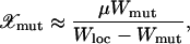
The process of shifting peaks via valley crossing (Wright 1932) or stochastic tunneling (Iwasa et al. 2004; Weinreich and Chao 2005) can happen if many mutants at Hamming distance unity from a local peak are available. While the Wrightian concept of valley crossing involves moving the whole population through a low-fitness sequence, the process of stochastic tunneling requires only the presence of a few low-fitness neighbors and we discuss this here. During the residence time of the population near the peak, a mutation–selection balance is reached between the peak genotype and its one-mutant neighbors. Then the average fraction of population at a given valley sequence with fitness W_mut can be estimated using the quasi-species equation, and one has

(11)

where W_loc is the fitness of the local peak. Clearly, the total number of mutants produced depends on the neighborhood of the local peak; if the fitness of the neighbors is much smaller than that of the local peak, then it is of the order NμL/W_loc where we have used that the average value of exponentially distributed variables is 1. Otherwise it is dominated by the population at the best one-mutant neighbor with fitness close to W_loc. In Figure 3, the sequence ranked 4 produced on average NLμ ∼ 10 mutants, while rank 5 produced a suite of ∼200 mutants, a lower bound (∼80) of which can be obtained by using (11) and the fitness W_mut of the rank 6 sequence, which is the fittest nearest neighbor of rank 5 sequence.

Since there are typically many low-fitness sequences available in the valley, it is likely that the population trapped at a local peak escapes due to a mutation in one of the NμL one-mutant neighbors. This gives the simple estimate of the tunneling time to be ∼(Nμ²L)⁻¹ ∼ 10³ for our choice of parameters. This in fact is a lower bound as the tunneling time depends inversely on the advantage conferred by the next local peak. An expression for the rate () to tunnel to a beneficial mutation via a deleterious one has been obtained in Iwasa et al. (2004), using a Moran process (also see Weinreich and Chao 2005). This is given by the product of three factors: average number of deleterious mutants produced, mutation probability with which a deleterious mutant mutates to an advantageous one, and the fixation probability that is the relative fitness difference between the final and initial mutants, finally yielding

(12)

where W_loc,{i,f} refers to fitness of the initial and the final local peaks. Inserting the fitness values of the two local peaks in question, T_tunnel turns out to be ∼3000, which is somewhat larger than that observed in Figure 3, top.

In Figure 3, center, although many mutants are available at the valley sequence ranked 6, the population could not tunnel through this sequence as it does not have a better neighbor other than sequence 5 itself. Instead a double mutation at t = 757 was responsible for escaping the local peak at the sequence ranked 5 to the next local peak with rank 2. Since the time T_double for the (desired) double mutation to occur in one generation is given by

(13)

(Iwasa et al. 2004; Weinreich and Chao 2005), it exceeds T_tunnel if W_mut ∼ W_loc, and in such a case, tunneling is the dominant mode of escaping the local peak. On the other hand, the valleys typically encountered in a rugged landscape are “deep” as and . In this situation, the population may attempt to hop across the valley; the probability for such an event is roughly given by Nμ² times the average number of fitter neighbors available at distance 2 away. The latter is simply (L²/2)Q(W(σ*)). Using , we again find that the timescale over which a double mutation can occur is of the same order as the tunneling time.

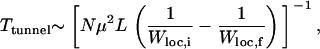
Crossover time:

We now estimate the time T_× at which the crossover from deterministic to stochastic evolution occurs using an argument employed previously by Krug and Karl (2003) and Jain and Krug (2005). We consider the evolution Equation 10 for the unnormalized population according to which the logarithmic population at a fit sequence increases linearly. Then the crossover time T_× at which the first local peak is reached can be approximated by the typical time at which the population at the first local peak (rank 5 in Figure 3) overtakes the population at the most populated sequence σ* (rank 28) at Hamming distance unity from it. This is given by

(14)

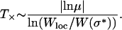
For the landscape used in Figure 3, the fitness W(σ*) ≈ 0.81 and W_loc ≈ 1.65 so that T_× works out to be ∼13 time steps, which is in reasonable agreement with the time at which X₅ appears. The dependence of T_× on L can be found by noting that generally the fitness ratio in the argument of the logarithm is close to unity, so that the logarithm can be expanded. The denominator then reduces to W_loc/W(σ*) − 1 ≈ 1/W(σ*) on using that the typical difference between two exponentially distributed independent random variables is equal to unity (David 1970; Sornette 2000). The fitness W(σ*) of the last-but-one most populated sequence in the quasi-species regime is expected to be of the same order as the fitness of the local peak, which increases as ln L. Thus for exponentially distributed fitness and d_eff = 1, the local quasi-species theory works over a timescale that increases as

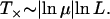(15)

Although we discussed mainly the case d_eff = 1 above, it is easy to see that for larger effective distance also, the local quasi-species theory will work up to a crossover time after which the population will get trapped at a “local peak” that does not have a better sequence available within Hamming distance d_eff and will have to wait for a rare mutation to find a better sequence. For , the crossover time can be easily generalized by approximating it by the time required for the last overtaking event to happen, which is given by Krug and Karl (2003) and Jain and Krug (2005):

(16)

Expanding the logarithm as above, and using that the peak genotype is the best among sequences, it follows that

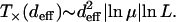(17)

Fully stochastic evolution:

We now turn to the regime when the effective distance is less than unity. Unlike in the previous cases, now the dynamics is stochastic at all times. The parameter d_eff < 1 implies that the average number of mutants Nμ produced at Hamming distance unity is also <1. Since the population is discrete, this number cannot be observed until time ∼(Nμ)⁻¹ when one mutant is produced at a given sequence. However, since the mutation probability is rotationally symmetric, a total of ∼LNμ new mutants at Hamming distance unity can be produced in one generation. The dynamics depend on whether the parameter LNμ is above or below unity, and we study these two cases in the following subsections. We focus mainly on the short time regime as the behavior at long times is expected to be similar to that discussed previously.

Clonal interference:

Figure 5 shows the temporal evolution of the population fraction for three different sampling noises (keeping the rest of the parameters the same). Clearly the population traces different trajectories in each case. In Figure 5, the population at σ⁽⁰⁾ produced a total of NLμ ∼ 1–2 mutants in one generation. Thus in this regime, the sequence space is very sparsely populated as only two to three genotypes are occupied. But since many [∼LQ(W(σ ⁽⁰⁾)) ∼ 13] of them are better than the parent, the population immediately begins the hill-climbing process. In Figure 5, top, the best one-mutant neighbor of σ⁽⁰⁾ with rank 4688 mutated once at t = 6 to move the population at a highly fit sequence ranked 159, which is also a local peak. In Figure 5, center, while most of the population climbed the nearest neighbor of the parent with rank 9195, an individual at a much lower rank 20,940 produced an offspring at 4117 at t = 5. Thus, due to the interference of rank 20,940 sequence, the population managed to access an even fitter sequence. After a single mutation at the genotype ranked 4117, the population reached a local peak with rank 1524 from where it escaped via double mutation. In Figure 5, bottom, at t = 5, the rank 14,622 neighbor of σ⁽⁰⁾ mutated once to populate a local peak with rank 2711. However, the population escaped this local peak by climbing a better local peak with rank 5 made available due to one mutation in sequence 14,622 at t = 7. In each case, since the selection coefficients involved are of order unity, the fitter mutants get fixed immediately and one can neglect the time to reach fixation.

Figure 5.—

Stochastic trajectories for L = 15, N = 2¹⁰, μ = 10⁻⁴ with Nμ ≈ 0.10 and LNμ ≈ 1.54. The population passes through different routes in each case right from the beginning and at short times, several mutants at constant Hamming distance are produced simultaneously. Only the mutants that achieve a fraction ≥0.005 are shown in the plot. (Top) All the mutants shown belong to the same lineage; (center and bottom) while a fit mutant is on its way to fixation, a split in the lineage produced an even better mutant, thus bypassing the former one.

In the preceding sections with , all the mutants are available within the occupied shells and the best among them becomes the most populated sequence σ*. However, for Nμ < 1, only a few randomly sampled sequences can get populated and as most of the genotypes available at Hamming distance 1 from σ⁽⁰⁾ are of comparable fitness, each of them can achieve a moderate population frequency. While the best among them has the highest chance of achieving majority status, the other mutants in the meanwhile can establish their own lineage by creating their own (small) suite of one-mutant neighbors. If a mutant better than the one that is currently going to fixation is produced, there is a competition and the latter is bypassed. This process is reminiscent of the bypassing discussed in quasi-species dynamics—in both cases, while a fit mutant is going to fixation, it may get bypassed by an even better one. However, while the set of mutants that will compete with each other in this manner is predetermined for large populations, here they are stochastically generated in time.

The competition between several beneficial mutations in an asexual population has been termed clonal interference (Gerrish and Lenski 1998). A quantitative criterion for the occurrence of clonal interference, adapted to the present situation, reads

(18)

(Wilke 2004), which is clearly satisfied in Figure 5. However, the usual view of clonal interference as an impediment to the simultaneous fixation of different beneficial mutations that slows down adaptation (Gerrish and Lenski 1998; Wilke 2004) relies on a situation in which the fitness effects are essentially additive, and hence strong (sign) epistasis is absent. In rugged fitness landscapes, on the other hand, the presence of several competing genotypes increases the likelihood of finding high-fitness genotypes. This effect is thus seen to speed up the adaptive process compared to the regime where beneficial mutations arise and fix sequentially, which we consider next.

Adaptive walk:

The above discussion, of course, is contingent on the fact that several genotypes are available to explore the landscape. We finally consider the case in which the rate LNμ at which the new mutants appear is very small. Then the time required to produce a new mutant is very large, and the competing mutants are not produced, enabling the population at the currently occupied genotype to reach a fraction unity. The population is thus localized at a single sequence at all times unlike in the previous cases where this happened only at long times. In Figure 6, the dynamics in the regime LNμ < 1 are shown for three different values of μ with fixed L and N. The effect of decreasing μ is similar to that in the quasi-species model in that the adaptive events are delayed and the polymorphism is reduced. Since the dynamics are now stochastic, the trajectories are different and an averaging is required to deduce the effect on fitness.

Figure 6.—

Population evolution when for L = 15, N = 2¹⁰ with μ = 10⁻⁵, 10⁻⁶, and 10⁻⁷ (top to bottom). The mutants with X_rank(σ) ≥ 0.005 are shown.

At short times, the number of occupied genotypes decreases with decreasing mutation probability. At late times, however, the population can be associated with a single sequence for large μ also due to a reduction in Q(W). In Figure 6, top, the left-hand side of (18) is ∼2, and correspondingly several genotypes coexist at early times. For , as in Figure 6, bottom, the population shifts as a whole by one Hamming distance. Since the mutation probability is small, to a first approximation, the population is likely to move only by one step and the hops to larger distances can be neglected. Thus, the population keeps moving one step uphill on the rugged landscape until it encounters a local peak whereupon this adaptive walk stops. The typical length of this walk is ln L ≈ 3 for L = 15 (Flyvbjerg and Lautrup 1992; Kauffman 1993). For μ = 10⁻⁷ in Figure 6, bottom, the population reaches the sequence with rank 2947, which is a local peak. The time to escape this sequence to a fitter one in the shell at Hamming distance 2 is of order (LNμ²)⁻¹ (as discussed above), which for our choice of parameters requires ∼10¹⁰ time steps. For small N and μ that we consider here, it may be possible for a valley mutant to get fixed before the next local peak does. This requires that the time to fix a valley mutant is smaller than the time ∼(Nμ)⁻¹ to produce its one-mutant neighbor with fitness W_loc,f (Carter and Wagner 2002; Nowak et al. 2004). The valley mutant fixation time is exponentially large in N if the mutant fitness 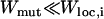, while it is of order N for the near neutral case. Clearly, the above requirement can be met only when the population escapes through a “shallow” valley, which is a rather unlikely scenario in a rugged landscape.

Before the population gets trapped at a local peak, the dynamics can be described by the mutational landscape model (Gillespie 1984), which applies to a genetically homogeneous population undergoing beneficial mutation with a very low probability. As pointed out in Orr (2002), the behavior of the population undergoing an adaptive walk is neither deterministic nor completely random in that each (better) mutant would be equally likely to get fixed. In fact, each one-mutant neighbor better than the currently occupied one has a probability to get fixed given by

(19)

where the sum is over the fitter nearest neighbors of σ⁽⁰⁾, and the unnormalized fixation probability is given by

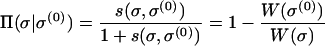(20)

for large N (Durrett 2002). In Figure 6, bottom, the probability for the sequence ranked 25,483 to get fixed is ≈0.049, which is almost half of the fixation probability ≈0.095 of the best available sequence with rank 4688.

DISCUSSION

In this article, we posed the question under what conditions biological evolution is predictable. To answer this, we studied the dynamics of a finite population N within a mutation–selection model defined on the space of binary genotype sequences of length L. This work thus considers L-loci models, unlike that of Rouzine et al. (2001), which focuses on the one-locus problem. Our simulations also differ from those of Wahl and Krakauer (2000), where the dynamics are described by the quasi-species Equation 1 as long as the population fraction X(σ, t) exceeds 1/N and if the fraction falls below this cutoff, an individual is added to sequence σ with a certain probability. We have instead simulated the full stochastic process defined by Wright–Fisher dynamics, which allows us to track the exact evolutionary path of any mutant. The fitness landscape under consideration is highly epistatic with many local optima.

We classified the various evolutionary regimes using a parameter d_eff defined in (6) that has been obtained under the assumption of strong selection. Usually the boundary between deterministic and stochastic evolution is defined by the product Nμ (Johnson et al. 1995; Wahl and Krakauer 2000; Rouzine et al. 2001); as most of these theories are based on one-locus models (Johnson et al. 1995; Rouzine et al. 2001), the description in terms of Nμ suffices. We are instead dealing with the whole sequence space in which mutations can occur to a distance greater than unity depending on the population size N and mutation probability μ. This requires a description in terms of the distance d_eff that measures the typical distance to which the mutants can spread. The boundary Nμ = 1 is included in our description as this corresponds to d_eff = 1. However, in contrast to the product Nμ, the logarithmic dependence of (6) implies that moderate changes in d_eff require enormous changes of N or μ.

Our conclusions summarized in Table 1 fall into three broad categories. The infinite-population case with d_eff = L is described by the deterministic quasi-species model (Eigen 1971). Given the fitness landscape and the starting point, one can predict the path taken by the initially unfit population to a peak in the landscape. For finite populations with , although the long time course is determined by stochastically occurring rare mutations, it is possible to predict the trajectory until a time T_× (Equation 17) that increases with L and N, using the deterministic prescription locally. We emphasize that the dynamics described by the local quasi-species theory that apply to shells of size d_eff centered about the current σ* are different from those of the quasi-species theory applied to the Hamming space restricted to the shells up to the one in which the local peak is located. This is simply because the initial population μ^d at the local peak in question can be <1/N. The intuitive picture provided by the local quasi-species theory is in fact equivalent to the description in Wahl and Krakauer (2000), where quasi-species is applied to full space provided the lower cutoff 1/N is imposed. The viewpoint that quasi-species dynamics can be useful in understanding the behavior of finite populations has been expressed by other authors also (see, for example, Wilke 2005).

TABLE 1.

Summary of regimes in evolution on rugged landscapes where d_eff = ln N/|ln μ|

	deff = L	1 ≤ deff < L	deff < 1
Behavior	Deterministic	Crossover deterministic → stochastic	Stochastic
Regime	Quasi-species	t < T×: local quasi-species	: clonal interference
		t > T×: valley crossing or hopping	LNμ < 1: adaptive walk

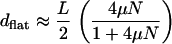
The local quasi-species description breaks down when the population fails to find a genotype better than the currently occupied one within distance d_eff. Then rare mutations (of the order ) that allow the population to access a distance >d_eff play an important role. On rugged landscapes, the population can escape this situation either by double mutations (for Nμ ∼ 1) or by tunneling through the low-fitness mutants (Iwasa et al. 2004; Weinreich and Chao 2005). Large populations are able to cross a fitness valley much more rapidly than expected on the basis of the adaptive walk picture, in which the fixation of a deleterious mutation is exponentially unlikely (van Nimwegen and Crutchfield 2000; Gavrilets 2004; Weinreich and Chao 2005). The reason is that in a large population the less-fit genotypes connecting the two fitness peaks are always present in some number, enabling the population to climb the new peak without ever in its entirety residing in the valley. This is similar to the peak shift mechanism found in the quasi-species model, where all possible mutants are always present in the population (Jain and Krug 2005, 2007).

To summarize, there is a crossover in the dynamics when from a deterministic quasi-species-type dynamics to stochastic dynamics in which stochastic escapes occur. For an RNA virus with typical population size N ∼ 10⁶ and mutation probability μ ∼ 10⁻³ per base per generation in a genome of ∼1000 bases (Lázaro 2007), these parameters give d_eff ≈ 2, which suggests that the local quasi-species dynamics operate in the finite viral populations for short times. This scenario is expected to hold good for human immunodeficiency virus also for which the product Nμ ∼ 1 (Rouzine and Coffin 1999).

For Nμ < 1, the dynamics are stochastic right from the start. The long-time dynamics are expected to be qualitatively similar to those discussed above. But the short-time dynamics differ considerably and depend on the number of one-mutant neighbors. While many analytical results are available for the adaptive walk limit (Gillespie 1984; Kauffman 1993), the parameter regime when NLμ is not too small on epistatic landscapes requires further attention. In experiments on Escherichia coli that has L ∼ 10⁶, μ ∼ 10⁻¹⁰, and typical colony sizes of order 10⁶, but , which hints at the stochastic nature of the bacterial evolution. This behavior has been seen in the experiments by the Lenski group in which the fitness of bacterial populations evolving under identical conditions diverged in time (Korona et al. 1994; Lenski and Travisano 1994).

In this article, we have provided a unified picture of the nature of the evolutionary process. As our models are defined on sequence space, this constitutes a step toward realistic modeling of the biological evolution occurring in the genotypic space. Inclusion of other relevant factors such as recombination could be the next step in our understanding of genetic evolution.

References

- Baake, E., and W. Gabriel, 2000. Biological evolution through mutation, selection, and drift: an introductory review, pp. 203–264 in Annual Reviews of Computational Physics VII, edited by D. Stauffer. World Scientific, Singapore.
- Burch, C. L., and L. Chao, 1999. Evolution by small steps and rugged landscapes in the RNA virus Φ6. Genetics 151: 921–927. [DOI] [PMC free article] [PubMed] [Google Scholar]
- Burch, C. L., and L. Chao, 2000. Evolvability of an RNA virus is determined by its mutational neighbourhood. Nature 406: 625–628. [DOI] [PubMed] [Google Scholar]
- Carter, A. J. R., and G. P. Wagner, 2002. Evolution of functionally conserved enhancers can be accelerated in large populations: a population-genetic model. Proc. R. Soc. Lond. Ser. B Biol. Sci. 269: 953–960. [DOI] [PMC free article] [PubMed] [Google Scholar]
- David, H. A., 1970. Order Statistics. Wiley, New York.
- Derrida, B., and L. Peliti, 1991. Evolution in a flat fitness landscape Bull. Math. Biol. 53: 355–382. [Google Scholar]
- Durrett, R., 2002. Probability Models for DNA Sequence Evolution. Springer, New York.
- Eigen, M., 1971. Self organization of matter and evolution of biological macromolecules. Naturwissenchaften 58: 465–523. [DOI] [PubMed] [Google Scholar]
- Eigen, M., J. McCaskill and P. Schuster, 1989. The molecular quasispecies. Adv. Chem. Phys. 75: 149–263. [Google Scholar]
- Elena, S. F., and R. E. Lenski, 2003. Evolution experiments with microorganisms: the dynamics and genetic bases of adaptation. Nat. Rev. Genet. 4: 457–469. [DOI] [PubMed] [Google Scholar]
- Elena, S. F., and R. Sanjuan, 2003. Climb every mountain? Science 302: 2074–2075. [DOI] [PubMed] [Google Scholar]
- Flyvbjerg, H., and B. Lautrup, 1992. Evolution in a rugged fitness landscape. Phys. Rev. A 46: 6714–6723. [DOI] [PubMed] [Google Scholar]
- Gavrilets, S., 2004. Fitness Landscapes and the Origin of Species. Princeton University Press, Princeton, NJ.
- Gerrish, P. J., and R. E. Lenski, 1998. The fate of competing beneficial mutations in an asexual population. Genetica 102: 127–144. [PubMed] [Google Scholar]
- Gillespie, J. H., 1984. Molecular evolution over the mutational landscape. Evolution 38: 1116–1129. [DOI] [PubMed] [Google Scholar]
- Haldane, J. B. S., 1927. A mathematical theory of natural and artificial selection. V. Proc. Camb. Philos. Soc. 23: 838–844. [Google Scholar]
- Higgs, P. G., 1994. Error thresholds and stationary mutant distributions in multi-locus diploid genetics models. Genet. Res. 63: 63–78. [Google Scholar]
- Iwasa, Y., F. Michor and M. A. Nowak, 2004. Stochastic tunnels in evolutionary dynamics. Genetics 166: 1571–1579. [DOI] [PMC free article] [PubMed] [Google Scholar]
- Jain, K., and J. Krug, 2005. Evolutionary trajectories in rugged fitness landscapes. J. Stat. Mech. Theor. Exp., P04008.
- Jain, K., and J. Krug, 2007. Adaptation in simple and complex fitness landscapes, in Structural Approaches to Sequence Evolution: Molecules, Networks and Populations, edited by U. Bastolla, M. Porto, H. Roman and M. Vendruscolo. Springer, Berlin (in press).
- Johnson, P. A., R. E. Lenski and F. C. Hoppensteadt, 1995. Theoretical analysis of divergence in mean fitness between initially identical populations. Proc. R. Soc. Lond. Ser. B 259: 125–130. [Google Scholar]
- Kauffman, S. A., 1993. The Origins of Order. Oxford University Press, New York.
- Kauffman, S. A., and S. Levin, 1987. Towards a general theory of adaptive walks on rugged landscapes. J. Theor. Biol. 128: 11–45. [DOI] [PubMed] [Google Scholar]
- Korona, R., C. H. Nakatsu, L. J. Forney and R. E. Lenski, 1994. Evidence for multiple adaptive peaks from populations of bacteria evolving in a structured habitat. Proc. Natl. Acad. Sci. USA 91: 9037–9041. [DOI] [PMC free article] [PubMed] [Google Scholar]
- Krug, J., and T. Halpin-Healy, 1993. Directed polymers in the presence of columnar disorder. J. Phys. I 3: 2179–2198. [Google Scholar]
- Krug, J., and K. Jain, 2005. Breaking records in the evolutionary race. Physica A 358: 1–9. [Google Scholar]
- Krug, J., and C. Karl, 2003. Punctuated evolution for the quasispecies model. Physica A 318: 137–143. [Google Scholar]
- Lázaro, E., 2007. Genetic variability in RNA viruses: consequences in epidemiology and in the development of new strategies for the extinction of infectivity, in Structural Approaches to Sequence Evolution: Molecules, Networks and Populations, edited by U. Bastolla, M. Porto, H. Roman and M. Vendruscolo. Springer, Berlin (in press).
- Lenski, R. E., and M. Travisano, 1994. Dynamics of adaptation and diversification-a 10,000 generation experiment with bacterial populations. Proc. Natl. Acad. Sci. USA 91: 6808–6814. [DOI] [PMC free article] [PubMed] [Google Scholar]
- Lunzer, M., S. P. Miller, R. Felsheim and A. M. Dean, 2005. The biochemical architecture of an ancient adaptive landscape. Science 310: 499–501. [DOI] [PubMed] [Google Scholar]
- Macken, C. A., and A. S. Perelson, 1989. Protein evolution on rugged landscapes. Proc. Natl. Acad. Sci. USA 86: 6191–6195.2762321 [Google Scholar]
- Macken, C. A., P. S. Hagan and A. S. Perelson, 1991. Evolutionary walks on rugged landscapes. SIAM J. Appl. Math. 51: 799–827. [Google Scholar]
- Nowak, M. A., F. Michor, N. L. Komarova and I. Iwasa, 2004. Evolutionary dynamics of tumor suppressor gene inactivation. Proc. Natl. Acad. Sci. USA 101: 10635–10638. [DOI] [PMC free article] [PubMed] [Google Scholar]
- Orr, H. A., 2002. The population genetics of adaptation: the adaptation of DNA sequences. Evolution 56: 1317–1330. [DOI] [PubMed] [Google Scholar]
- Rouzine, I. M., and J. M. Coffin, 1999. Linkage disequilibrium test implies a large effective population number for HIV in vivo. Proc. Natl. Acad. Sci. USA 96: 10758–10763. [DOI] [PMC free article] [PubMed] [Google Scholar]
- Rouzine, I. M., A. Rodrigo and J. M. Coffin, 2001. Transition between stochastic evolution and deterministic evolution in the presence of selection: general theory and application to virology. Microbiol. Mol. Biol. Rev. 65: 151–185. [DOI] [PMC free article] [PubMed] [Google Scholar]
- Sire, C., S. Majumdar and D. S. Dean, 2006. Exact solution of a model of time-dependent evolutionary dynamics in a rugged fitness landscape. J. Stat. Mech., L07001.
- Sornette, D., 2000. Critical Phenomena in Natural Sciences. Springer, Berlin.
- van Nimwegen, E., and J. P. Crutchfield, 2000. Metastable evolutionary dynamics: Crossing fitness barriers or escaping via neutral paths? Bull. Math. Biol. 62: 799–848. [DOI] [PubMed] [Google Scholar]
- Wahl, L. M., and D. C. Krakauer, 2000. Models of experimental evolution: the role of genetic chance and selective necessity. Genetics 156: 1437–1448. [DOI] [PMC free article] [PubMed] [Google Scholar]
- Weinreich, D. M., and L. Chao, 2005. Rapid evolutionary escape by large populations from local fitness peaks is likely in nature. Evolution 59: 1175–1182. [PubMed] [Google Scholar]
- Weinreich, D. M., R. A. Watson and L. Chao, 2005. Sign epistasis and genetic constraint on evolutionary trajectories. Evolution 59: 1165–1174. [PubMed] [Google Scholar]
- Weinreich, D. M., N. F. Delaney, M. A. DePristo and D. L. Hartl, 2006. Darwinian evolution can follow only very few mutational paths to fitter proteins. Science 312: 111–114. [DOI] [PubMed] [Google Scholar]
- Whitlock, M. C., P. C. Phillips, F. B.-G. Moore and S. J. Tonsor, 1995. Multiple fitness peaks and epistasis. Annu. Rev. Ecol. Syst. 26: 601–629. [Google Scholar]
- Wilke, C. O., 2004. The speed of adaptation in large asexual populations. Genetics 167: 2045–2053. [DOI] [PMC free article] [PubMed] [Google Scholar]
- Wilke, C. O., 2005. Quasispecies theory in the context of population genetics. BMC Evol. Biol. 5: 44. [DOI] [PMC free article] [PubMed] [Google Scholar]
- Wright, S., 1932. The roles of mutation, inbreeding, crossbreeding and selection in evolution, pp. 356–366 in Proceedings of the Sixth International Congress of Genetics, edited by D. F. Jones. Brooklyn Botanic Garden, Menasha, WI.
- Yedid, G., and G. Bell, 2002. Macroevolution simulated with autonomously replicating computer programs. Nature 420: 810–812. [DOI] [PubMed] [Google Scholar]
- Zhang, Y.-C., 1997. Quasispecies evolution of finite populations. Phys. Rev. E 55: R3817–R3819. [Google Scholar]