Inference of Bacterial Microevolution Using Multilocus Sequence Data

Abstract

We describe a model-based method for using multilocus sequence data to infer the clonal relationships of bacteria and the chromosomal position of homologous recombination events that disrupt a clonal pattern of inheritance. The key assumption of our model is that recombination events introduce a constant rate of substitutions to a contiguous region of sequence. The method is applicable both to multilocus sequence typing (MLST) data from a few loci and to alignments of multiple bacterial genomes. It can be used to decide whether a subset of isolates share common ancestry, to estimate the age of the common ancestor, and hence to address a variety of epidemiological and ecological questions that hinge on the pattern of bacterial spread. It should also be useful in associating particular genetic events with the changes in phenotype that they cause. We show that the model outperforms existing methods of subdividing recombinogenic bacteria using MLST data and provide examples from Salmonella and Bacillus. The software used in this article, ClonalFrame, is available from http://bacteria.stats.ox.ac.uk/.

BACTERIA reproduce clonally but their genomes evolve by a variety of mechanisms, including point mutation, genome rearrangement, deletion, duplication, bacteriophage lysogeny, gene degradation, transposition, slippage mutation in DNA sequence repeats, and homologous and nonhomologous recombination (Maynard Smith et al. 1993; Feil et al. 1999, 2000; Lawrence and Hendrickson 2003). Recombination can occur when bacterial DNA enters the host cell via conjugation (which requires cell-to-cell contact between a donor and a receiver), transformation (uptake of naked DNA that remains from the lysis of another cell), or transduction (which involves packing of host DNA in a phage and release in the receiver).

The variety of evolutionary mechanisms by which bacteria evolve can pose problems when attempting to infer relationships between strains. Clonal relationships can be represented by a genealogy, which is a tree where each leaf is a member of the sample and each internal node is the most recent common ancestor of the descendant strains. Each node is associated with a time before the present when that ancestor divided. Many methods for inferring these relationships rely on DNA sequence differences. Point mutations happen approximately randomly and independently and thus, in the absence of other processes, would allow accurate reconstruction of clonal relationships using standard phylogenetic methods (Felsenstein 1989; Swofford 2002; Drummond and Rambaut 2003). However, even in “housekeeping genes” that are required for metabolic function, so that gross changes in sequence such as insertions or deletions are likely to be lethal and therefore rarely observed, homologous recombination with other bacteria from the same population can change several nucleotides at once (Milkman and Crawford 1983). These events are overweighted by nucleotide-based phylogenetic methods in comparison to point mutations, which can lead to inaccurate genealogies being inferred (Schierup and Hein 2000).

The necessity to account for recombination as well as point mutation in genealogical inference has led to the development of sequencing strategies such as multilocus sequence typing (MLST), which involves sequencing a handful (typically seven) of fragments from housekeeping genes that are each sufficiently far apart on the chromosome of the type strain that it would be unlikely for more than one of them to be affected by a single recombination event (Maiden et al. 1998). It has also led to the use of allele designations for each unique sequence at each locus rather than the sequence itself. Alleles are considered to be equally distinct from each other whether they differ at one nucleotide position or at many with the consequence that recombination and mutation events are given similar weight in analysis. A variety of methods have been adapted, and new ones such as BURST have been developed, to analyze genetic relationships using allele designations (Jolley et al. 2001; Feil et al. 2004; Spratt et al. 2004).

Allele-based methods have important limitations. Alleles that differ at one or two nucleotides can provide evidence for a higher degree of relatedness for the strains that carry them than alleles that differ by many. For example, if recombination were rare, and a strain differed from a second one by one or two nucleotide differences at six of seven loci and by many nucleotides at the seventh one then the two strains would be classified as unrelated by allele-based methods despite the clear evidence for a relatively recent common ancestor provided by the six similar loci. Additionally, variation in relatedness within each sequence fragment is ignored. A half fragment of identical sequence provides evidence of relatedness even if the other half contains several nucleotide differences because this spatial pattern will most likely have been caused by a homologous recombination event whose boundary occurred at the middle of the fragment. Allele-based methods are thus more suited to exploratory data analysis than to fine statistical inference. Ultimately, we are interested in patterns of relatedness for entire bacterial genomes and therefore would like to dispense with arbitrary boundaries between loci and instead infer the beginning and end points of each homologous recombination event.

Here we describe a statistical approach for inferring bacterial clonal relationships on the basis of DNA sequences that accounts for both point mutation and homologous recombination. In bacteria, each recombination event affects a contiguous region of sequence, but leaves the remainder of the circular chromosome unchanged. In the language of eukaryotic geneticists, we therefore need to model gene conversion-like events, but not crossovers. Our method estimates the extent of the clonal frame for each branch of the genealogy, which is the subset of the genome that has not undergone recombination (Milkman and Bridges 1990). Our approach is model based in the sense that it attempts to infer the parameters and events in the evolutionary process that led to the observed pattern of DNA sequence variation. However, our method does not attempt to model the origin of the DNA imported in homologous recombination events, instead assuming that imported stretches differ from the sequence they replace at a constant proportion of nucleotides, ν. ν is estimated from the data but does not have a straightforward biological interpretation.

We do not attempt to model the origin of imports for two reasons. First, a full description of the ancestral relationships of all the DNA in a sample, the ancestral recombination graph (ARG), is extremely complex (Griffiths and Marjoram 1996). This complexity makes it computationally challenging to perform inference of the ARG even for modestly sized data sets in which the sample can be assumed to come from a closed, homogenous population in which recombination takes place at a uniform rate between all pairs of strains (McVean and Cardin 2005). Second, bacteria are often more promiscuous than eukaryotes, occasionally importing DNA from different species (e.g., Dingle et al. 2005) or even genera (Ochman et al. 2000), making the standard assumption of a closed, homogeneous population particularly unrealistic. Ignoring interpopulation events is problematic even if they are rare because these events can be responsible for a large number of nucleotide differences. Our method avoids both of these problems. However, because it does not look for potential sources of descent for each stretch of DNA, it tends to underestimate the number of recombination events that have taken place (see results below). Nevertheless, it is still able to infer genealogies more accurately than existing methods, with an algorithm that is fast enough to be applied to multiple bacterial genomes.

We perform inference in a Bayesian framework, which means that we need to specify a prior for the genealogical process that defines the probability of any genealogy before observing the data. We assume a standard neutral coalescent model (Kingman 1982), which is equivalent to assuming that the bacteria in the sample come from a constant-sized population in which each bacterium is equally likely to reproduce, irrespective of its previous history. More details about the coalescent can be found, for example, in Donnelly and Tavaré (1995). A coalescent prior has the advantage of tractability and simplicity. However, it has been shown that for many bacterial populations, there is an excess of isolates with identical allelic profiles, in comparison to neutral expectations (Fraser et al. 2005; Jolley et al. 2005). Since bacteria do not disperse at each replication, different growth conditions in different physical locations could introduce local correlations in the genealogy. The geographical and temporal extent of these correlations has not been established for any bacterial species and other factors such as selection and demography can also cause deviations from neutral expectation. These deviations might introduce biases in the genealogy produced by our method. Fortunately new genotyping technologies will allow population variation to be surveyed at a genomic scale. Such data have the potential to provide a great deal of information on the shape of the genealogy, which reduces the importance of the prior and will ultimately reveal the causes of the deviations from neutrality that have been observed.

MODEL AND METHODS

We now provide a more detailed description of our modeling assumptions and the algorithms used to perform inference. The mathematical symbols used and their meanings are summarized in Table 1.

TABLE 1.

Symbols used

Symbol	Description
Data
𝒜	Aligned sequence data
N	Number of sequences
L	Total length of the sequences
b	Number of blocks in the alignment
{si}i=1,…,b	Size of the ith block
Model parameters
𝒯	Genealogy
ℛ	Locations of recombination events associated with the branches of the genealogy
𝒞	Ancestral sequences for the internal nodes of the genealogy
ℳ	Model parameters: ν, R, δ, θ
θ/2	Rate of mutation on the branches of the genealogy
R/2	Rate of recombination on the branches of the genealogy
ν	Rate of nucleotide differences in the recombined stretches
δ	Mean of the exponential distribution modeling the length of recombinant segments
{ti}i=1,…,N−1	Age of the ith coalescent event (looking back in time)
u	Probability that a specific recombination event starts at any given site within a block
u′	Probability that a specific recombination event starts at the beginning of a given block
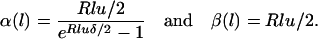
α(l)	Parameter of the exponential distribution modeling the length of imported regions for a branch of length l
β(l)	Parameter of the exponential distribution modeling the length of nonimported regions for a branch of length l

Model:

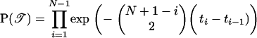
We perform statistical inference assuming that the clonal genealogy and the sequences on each node have been generated by the probabilistic model described in this section and summarized in Figure 1. Let t₁, … , t_N−1 specify the times before the present at which branching takes place in the genealogy, with t₁ < t₂ < . . . < t_N−1 and let t₀ = 0. The assumption of a coalescent prior means that for all i ∈ [1, … , N − 1], the difference t_i − t_i−1 is exponentially distributed with mean 2/(N − i)(N − i + 1). The prior probability for the entire genealogy, 𝒯, is equal to the product of probability of all N − 1 branching events,

(1)

Figure 1.—

Illustration of the model. Two blocks (horizontal lines) evolve by point mutation (black crosses) and recombination from an unmodeled origin (colored arrows, inducing the substitutions marked by colored crosses). corresponds to the observed sequences and corresponds to the sequences at internal nodes.

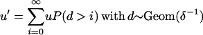
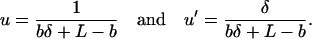
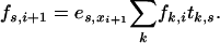
Each sequence is assumed to consist of b blocks of size (s₁, … , s_b), with . Each site of the sequence at the topmost node of the tree is equally likely to be one of the four bases A, C, G, and T. The sequence associated with each daughter node is generated by the combined effects of recombination and mutation. Recombination happens between each node as a Poisson process of rate R/2, so that for a branch of length l, the total number of recombination events is Poisson distributed with mean Rl/2. Each recombination event affects a contiguous stretch of the sequence of the daughter node. Only a small proportion of the chromosome may be available in the alignment and we model only events that affect this subset while assuming that events occur uniformly on the whole chromosome. To do this, we make the simplifying assumptions that blocks are distant enough from each other that each recombination event affects one and only one block and that recombination events are equally likely to start at any site on the genome. The total length of a recombination event is assumed to be geometrically distributed with mean δ. For any given recombination event that affects a given block, the probability that it starts at any nucleotide in the block except for the first is identical and is denoted u. The probability that the observed beginning of the event is at the first nucleotide of a block is higher and equal to

(2)

(3)

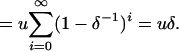
Summing over all possible sites, we get

(4)

Within the recombined regions (which are affected by at least one recombination), the daughter sequence is altered with constant rate ν. Within the nonrecombined regions the daughter sequence at each nucleotide is altered with probability θl/2L on the branches of the genealogy. Altered nucleotides are replaced according to the model of Jukes and Cantor (1969), where all substitutions are equally likely.

Inference:

Given the data 𝒜, which consist of the N sequences at the leaves of the genealogy, we wish to infer the genealogy, 𝒯; the sequences at each of the internal nodes, 𝒞; the position of the recombined regions in each of the branches of the genealogy, ℛ; and the four model parameters . In formal terms, we wish to calculate the posterior of all these terms given the data, . While it is not possible to compute this distribution exactly, it is possible to use Markov chain Monte Carlo (MCMC) to obtain an approximate sample (Gilks et al. 1998). See, for example, Pritchard et al. (2000) for another application of MCMC to population genetics inference.

MCMC involves updating subsets of the parameters, conditional on the values of the others. To do so, we make use of the following decomposition:

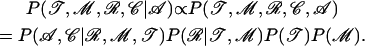(5)

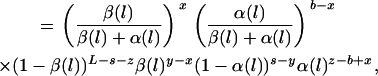
is the prior probability of the genealogy, which is independent of other parameters and given by Equation 1. is the prior probability of the model parameters that are detailed in appendix c. is the prior probability of the locations of the recombined regions for each branch of the genealogy. The locations of these regions are independent from branch to branch and can be calculated block-by-block using a Markovian approximation detailed in appendix a, where the lengths of recombined and nonrecombined regions are assumed to be exponentially distributed with parameters α(l) and β(l), respectively. Each branch has an associated map of imported regions, r, where r_i,j = 1 when the jth position of the ith block of r is imported and r_i,j = 0 otherwise. The prior distribution of r for a branch of length l is given by

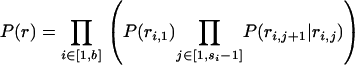(6)

(7)

where 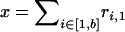is the number of blocks starting in imported state, y is the total number of imported regions of r, z is the total number of nonimported regions of r, and .

is proportional to the product for each branch of 𝒯 of the probability to obtain the sequence at the bottom of the branch given the sequence at the top of the branch and the location of imports for the branch. For a branch a of length l this is equal to

(8)

where x is the number of nonidentical sites in nonimported regions, y the number of identical sites in nonimported regions, z the number of nonidentical sites in imported regions, and L − x − y − z the number of identical sites in imported regions.

We are now in a position to outline updates for the elements of 𝒞, ℛ, 𝒯, and ℳ. The model parameters ℳ and the ages of the nodes of the genealogy are updated using the Metropolis–Hastings algorithm as described in appendix c. We also designed an additional update to deal with missing data presented in appendix d.

The ancestral sequences and maps of imports are updated node-by-node. We outline the update for a nonroot internal node n of the tree 𝒯. A similar update is used for the root. The locations of the recombined regions are highly correlated with the ancestral sequences of the nodes, so to achieve better mixing of the Markov chain we update the location of recombination events of the branch above and the two branches below each internal node simultaneously with the ancestral sequence associated to n. This is done using the forward–backward algorithm as detailed in appendix b.

The branching of the genealogy is updated by a version of the branch-swapping algorithm of Wilson and Balding (1998). A nonroot internal node x is chosen uniformly as well as a node y and we propose to reconnect x on the branch above y. y is chosen according to the procedure adopted by Wilson and Balding (1998). The age of the newly created node n is drawn uniformly from [max(t_x, t_y), t_z] if y has a father z and from [t_y, t_y + 1] if y is the root. To calculate the ancestral sequence and location of imports for the new node n, we apply the forward–backward algorithm described in appendix b to the node n. The move is accepted according to the Metropolis–Hastings acceptance ratio

(9)

where the ratio of posterior probabilities can be calculated using Equation 5 and is the probability to propose the new parameters and is given by

(10)

where Q(y | x) is the probability to propose y given x as described by Wilson and Balding (1998); Q(age) is the probability that the age of n was proposed, which is equal to 1 if y is the root and to 1/(t_z − max(t_x, t_y)) otherwise; and Q(HMM) (hidden Markov model, HMM) is the probability that the forward–backward algorithm returned the given ancestral sequence for n and location of imports for n and its children x and y.

In all of the examples shown, each iteration of the MCMC algorithm updates the ancestral sequence and associated location of imported regions for each internal node once as described in appendix b. Updates are also performed for the age of each node; for the values θ, R, ν, and δ; and for the nucleotide sequence of any missing data. A single attempt is also made to change the topology 𝒯 using the branch-swapping algorithm. However, experimentation has shown that the mixing is improved by attempting several topology updates per iteration, especially for large data sets. Convergence and mixing properties were assessed by monitoring parameters and comparing runs with different starting conditions (Gelman and Rubin 1992).

APPLICATIONS TO DATA

Detection of imports from an external origin:

The simplest use of our method is to detect genetic imports affecting closely related strains, from sources that are external to the data set. Our model is particularly well suited to this scenario because of the assumption that all recombination events introduce novel polymorphisms. Even if this assumption that imported stretches contain a constant rate ν of new polymorphisms is not met exactly, it should still be relatively easy for the model to distinguish imports from point mutations, which will be scattered and rare.

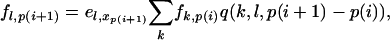
This use is illustrated in Figure 2 for four genomes of Salmonella enterica, serovar Typhimurium [LT2 is published in McClelland et al. 2001; DT2, DT104, and SL1344 are unpublished data from the Sanger Institute (J. Parkhill and N. Thomson)]. An alignment of the four genomes was built using Mauve (Darling et al. 2004): 57 sequence stretches were found that are locally colinear in all four genomes, making up an alignment of total length L = 4,957,309 bp. Each of these was input as a block in our program. Our program was run for 10,000 iterations (including 5000 burn-in iterations), which required 72 hr on a desktop computer. Results were highly replicable between different runs.

Figure 2.—

Application to whole genomes of Salmonella enterica serovar Typhimurium. (A) A neighbor-joining tree; (B) a UPGMA tree; (C) a majority-rule consensus tree based on the output of BEAST (Drummond and Rambaut 2003); (D) a majority-rule consensus tree based on the posterior distribution of genealogies inferred by our method. Black numbers above each branch indicate observed/expected numbers of mutations, while red numbers below the branch indicate the equivalent values for recombination events followed by the total number of substitutions caused. The scale is the same for all three trees and is proportional to the expected number of mutations in each branch in D given the inferred values of θ and 𝒯. (E) Highlights the events on each branch of D. Each row represents 300,000 bp, with recombined regions in red and point mutations in green. (F) Three regions containing imports, with crosses indicating substitutions and the red line indicating probability for each nucleotide to have recombined. The location of the beginning and end of each region is indicated in kilobase pairs.

Our method (Figure 2D) produces a tree with shorter branches than those of neighbor joining (Figure 2A, with root chosen arbitrarily), UPGMA (Figure 2B), or BEAST (Figure 2C) (Drummond and Rambaut 2003). One reason is that our method identified 50 imported regions with an estimated mean length δ of 800 bp that have introduced a total of 872 substitutions. These events (Figure 2E) are in most cases visually obvious, introducing a much higher number of substitutions than observed in the clonal frame (Figure 2F). ν, the rate of differences introduced by recombination is estimated between 1.2 and 1.4%. This value is close to the average number of differences between strains of S. enterica based on MLST data (Falush et al. 2006) and much higher than the maximum rate of mutations inferred in the clonal frame of any branch of the genealogy, which is 0.01%, implying that the method should successfully identify imports from unrelated S. enterica as long as they are >200–300 bp in length.

Our analysis allows us to make a detailed reconstruction of the events involved in the divergence of these four strains. First, it shows that LT2 and DT104 are the most closely related, sharing 141 point mutations and four imports. Second, the genealogy is star-like in shape, splitting into four lineages soon after they all shared a common ancestor. This pattern is unlikely under the coalescent prior. Specifically, the ratio of the last and first coalescence times in the posterior is higher than that in a random coalescent genealogy 98% of the time. Our program inferred this pattern because most of the polymorphic sites in the data set are unique to one strain. This pattern is consistent with a rapid clonal expansion of the most recent common ancestor of these Typhimurium, which perhaps coincided with adaptation to its current niche in farm animals. Third, there is clear evidence for a higher number of mutations in the DT2 lineage, with SL1344 also evolving more slowly than the other strains, since the observed number of mutations in both lineages is significantly different from what is expected given a constant mutation rate. The elevated rate of change is not due to relaxed selection, since the ratio of synonymous to nonsynonymous mutations does not differ significantly between lineages (data not shown). Thus, the mutation rate has changed at least twice during a relatively short evolutionary history.

Our algorithm was, however, unable to infer which pair of LT2, DT104, and the ancestor of DT2 and SL1344 is most closely related. This is indicated by a three-way branching at the top of the consensus tree shown in Figure 2D, which means that there is not a pair of strains that is most closely related in 50% of the posterior sample of genealogies produced by the MCMC. The inability to infer this branching pattern despite having data from the entire genome is partly due to the star-shaped genealogy but also to the intrinsic difficulty of resolving the location and sequence of the root of a tree.

Application to simulated data from a closed population:

A more ambitious use of the method is to attempt to define the clonal relationships and imports for a sample from an entire bacterial species. The assumptions of the model fit less well since in many instances recombination will reassort existing polymorphisms rather than introduce novel ones. In addition, the deeper branches in the genealogy might be difficult or impossible to resolve accurately, especially if there has been substantial recombination so that most of the genome of each strain has been exchanged since they shared a common ancestor. Finally, imports from closely related strains might be difficult to distinguish from mutation, particularly for the longer branches, so that the value of ν becomes more important in the inference.

Analysis of simulated data sets shows that despite these potential difficulties our model provides useful results and outperforms existing methods of subdividing bacterial populations. To evaluate the performance of our algorithm we simulated ARGs using the algorithm described in Hudson (1983) but with gene conversion rather than crossing over. The simulation parameters were chosen to approximately mimic MLST data, with seven unlinked fragments of 500 bp each for N = 100 isolates and an average tract length of δ = 1000 (Tables 2 and 3). For each data set, 100,000 iterations of our program were performed (including 50,000 burn-in interations), which required ∼12 hr on a desktop computer. Instead of checking convergence for each run we assess the validity of the results by comparison with the true history.

TABLE 2.

Comparison of the efficiency and accuracy of UPGMA using site-by-site and gene-by-gene bootstrapping, BURST, and our method on simulated data

	Parameters		UPGMAa		UPGMAb		BURST		Our program
Simulation no.	θ/L (×100)	ρ	Efficiency	Accuracy	Efficiency	Accuracy	Efficiency	Accuracy	Efficiency	Accuracy
1	0.2	0	0.16	0.94	0.19	0.90	0.11	0.83	0.17	0.95
2	1.0	0	0.42	0.91	0.44	0.91	0.20	0.84	0.42	0.94
3	5.0	0	0.57	0.85	0.57	0.82	0.15	0.86	0.75	0.94
4	0.2	1	0.14	1.00	0.14	1.00	0.11	0.84	0.19	0.94
5	1.0	1	0.37	0.86	0.38	0.84	0.19	0.82	0.43	0.95
6	5.0	1	0.65	0.85	0.67	0.87	0.15	0.85	0.73	0.93
7	0.2	5	0.14	0.87	0.15	0.88	0.12	0.86	0.19	0.86
8	1.0	5	0.35	0.79	0.38	0.76	0.18	0.80	0.40	0.86
9	5.0	5	0.57	0.74	0.58	0.77	0.14	0.88	0.70	0.90
10	0.2	10	0.21	0.67	0.17	0.85	0.14	0.80	0.19	0.81
11	1.0	10	0.33	0.66	0.34	0.73	0.18	0.80	0.39	0.84
12	5.0	10	0.70	0.85	0.70	0.87	0.16	0.91	0.71	0.89

^aSite-by-site bootstrapping.

^bGene-by-gene bootstrapping.

TABLE 3.

Comparison of the efficiency and accuracy of our method for different sizes of simulated data

	7 × 500 bp				14 × 500 bp
Simulation no.	θ/L (×100)	ρ	Efficiency	Accuracy	θ/L (×100)	ρ	Efficiency	Accuracy
1	0.2	0	0.17	0.95	0.2	0	0.28	0.96
2	1.0	0	0.42	0.94	1.0	0	0.58	0.94
3	5.0	0	0.75	0.94	5.0	0	0.84	0.96
4	0.2	1	0.19	0.94	0.2	2	0.23	0.96
5	1.0	1	0.43	0.95	1.0	2	0.54	0.96
6	5.0	1	0.73	0.93	5.0	2	0.84	0.94
7	0.2	5	0.19	0.86	0.2	10	0.27	0.86
8	1.0	5	0.40	0.86	1.0	10	0.53	0.90
9	5.0	5	0.70	0.90	5.0	10	0.79	0.91

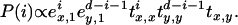
Figure 3 compares our method and eBURST (Feil et al. 2004), an implementation of the BURST algorithm, for one example with θ = 0.2 per site, and ρ = 5 for the entire data set. In this example, it is clearly not going to be possible to infer every branch of the genealogy let alone to accurately estimate each branch length (both shown in Figure 3A) because the 100 isolates have only 27 sequence types between them. We handle the statistical uncertainty by retaining only branches that are supported in a majority-rule consensus tree (Bryant 1997) on the basis of the posterior probability for the genealogy and using the posterior mean for the length of each supported branch (Figure 3B). Our algorithm both correctly captures the overall structure of the tree and correctly infers the sequence types (STs) of most internal nodes (shown in italics on each branch, with x denoting an ST that is not found in extant strains). One of the few errors is that the strain with ST 20 is not correctly grouped with STs 7 and 4 on the genealogy inferred by our method. An explanation can be found by looking at the sequence types of the ancestral nodes of the real topology: ST 20 was in fact the type of the most recent common ancestor of more than half of the sample. This type disappeared by mutation and recombination, but reappeared later once due to recombination. Our program has correctly inferred that the type of the most recent common ancestor (MRCA) of STs 1 and 3 was 20 and therefore clustered the observed isolate of type 20 at that point in the tree, which is the most parsimonious explanation for the observed data but not the correct one in this case.

Figure 3.—

Application to simulated MLST data. (A) The true clonal genealogy; (B) the genealogy inferred by our program; (C) a UPGMA tree. The genealogies were drawn using the radial tree option of Mega (Kumar et al. 2001) and share a common scale. STs of internal nodes are indicated in italics in A and B, with x indicating an ST that does not occur in the sample. STs are indicated in regular type, with the size of the font approximately proportional to the number of strains represented. (D) The output of eBURST; (E) a network representation of our output using Graphviz (Gansner and North 2000). The network shows inferred ancestral nodes in black and the location of isolates in red, with each red line indicating a single isolate. Each isolate has the genotype of the node it is connected to, unless otherwise indicated. Nodes whose ST is not found among isolates are shown as an empty circle. The ancestral node of each network component is indicated by a thicker circle.

A UPGMA tree (Figure 3C) correctly captures most of the branch structure of the tree but gets the branching order of the deepest clades wrong (i.e., in the true tree ST 3 is more closely related to ST 2 than to ST 11 while the UPGMA tree indicates the opposite). Another issue is that many branch lengths are exaggerated (e.g., ST 21). Indeed the correlation coefficient between the time of divergence between pairs of strains and their number of nucleotide differences on which UPGMA is based is 0.91, whereas the times inferred by our method have a correlation coefficient of 0.97 with the true values. The UPGMA tree also does not make it explicit which STs constitute monophyletic clusters (e.g., ST 11 does not since it occurs in more than one place in the true tree).

eBURST (Figure 3D) correctly identifies many of the subdivisions at the tips of the tree. However, it fails to identify any of the deep nodes in the tree, for example, failing to indicate that ST 11 and ST 14 are related to each other, and also fails to find close relatives for ST 25 or ST 26. Moreover, although it sometimes assigns ancestral sequences to particular lineages these assignments are not particularly accurate (for example, ST 23 is not ancestral to ST 3). A similar network representation of the consensus genealogy (without estimated branch lengths) obtained using our method is shown in Figure 3E. This representation, which should be particularly useful for large data sets, makes it explicit that some STs (for example, ST 2) probably occur in more than one location in the true genealogy, while others probably form a single cluster (such as ST 17). Indeed in this case, inspection of the true genealogy shows that some ST 2 isolates are more closely related to ST 17 isolates than they are to some of the other ST 2's.

More formally, two types of error can be identified for the branching pattern. An error of type A happens, for example, for STs 1, 9, and 12, where the clustering of these three STs is correctly identified by our method, but the details of how these three STs relate to each other was not inferred. We call efficiency the ratio of numbers of correctly inferred clusters and clusters present in the data (this second number being always equal to N − 1). An error of type B happens, for example, for ST 20, which is not inferred to be a close relative of 4 as it should be, causing the cluster containing STs 4 and 7 to be wrong. We call accuracy the proportion of inferred clusters that are correct. For this example the efficiency of our program is 18% and its accuracy is 90%. Exactly the same method can be used to measure the performance of BURST (which we reimplemented ourselves for the purpose of comparison). We interpreted BURST output as a genealogy analogous to ours. Specifically we assume that only STs at the tips of each complex and groups of STs that form a single clade radiating from the ancestral ST are predicted to be monophyletic. According to these criteria, the efficiency of BURST is 13% and its accuracy is 68%. The alternative assumption that each ST constitutes a monophyletic lineage gives an increase in efficiency, but at the expense of a large decrease in accuracy (data not shown).

We have performed simulations of 10 ARGs similar to the one presented above for a range of parameter combinations (θ, ρ), which shows that our algorithm provides accurate subdivisions and outperforms existing methods (Table 2). BURST has consistent accuracy of 80–91% for all parameter combinations we explored but never infers >20% of the nodes correctly, even when there are a large number of mutations on the tree, so that the data are potentially highly informative about relationships between strains.

UPGMA trees can be bootstrapped either site-by-site or gene-by-gene. The latter takes into account the property that recombination can import an entire gene that may look similar to the sequence of another strain. Gene-by-gene bootstrapping performs more accurately for high recombination rates but both methods generally underperform our program in both accuracy and efficiency. The efficiency of our method is significantly increased for all parameter combinations by doubling the number of loci to 14, showing that additional sequencing is likely to be effective in providing additional resolution (Table 3).

In general, the performance of our method increases with θ and decreases with ρ. For low values of θ (simulations 1, 4, 7, and 10), the accuracy and efficiency of our program is only slightly better than that of bootstrapped UPGMA trees. However, for higher values of θ (simulations 3, 6, 9, and 12), our program outperforms bootstrapped UPGMA trees both in accuracy and in efficiency by up to 10% (simulations 3 and 9).

Our model can also be used to estimate model parameters (Table 4). It provides accurate and approximately unbiased estimates of θ and the size of imported chunks, δ. Estimates for the recombination rate ρ are poor when ρ and θ are low (simulations 1–7 and 10) but become better for higher values of these two parameters (simulations 9 and 12).

TABLE 4.

Parameter estimation on simulated data

	Parameters		θ/L			R			δ−1
Simulation no.	θ/L (×100)	ρ	Mean	SD	Right	Mean	SD	Right	Mean	SD	Right
1	0.2	0	0.17	0.05	10/10	0.03	0.06	0/10	0.014	0.018	9/10
2	1.0	0	0.98	0.14	10/10	0.10	0.12	0/10	0.015	0.017	9/10
3	5.0	0	5.01	0.57	10/10	0.06	0.08	0/10	0.021	0.022	9/10
4	0.2	1	0.24	0.05	10/10	0.17	0.35	0/10	0.011	0.014	8/10
5	1.0	1	0.97	0.17	10/10	1.01	0.41	1/10	0.012	0.014	9/10
6	5.0	1	5.09	0.57	9/10	2.98	0.42	3/10	0.004	0.004	8/10
7	0.2	5	0.22	0.06	10/10	1.27	1.16	0/10	0.012	0.015	10/10
8	1.0	5	1.03	0.16	10/10	3.36	0.81	4/10	0.001	0.001	7/10
9	5.0	5	5.06	0.56	10/10	4.80	0.98	6/10	0.002	0.001	7/10
10	0.2	10	0.2	0.06	8/10	12.92	2.1	0/10	0.010	0.013	7/10
11	1.0	10	1.03	0.16	9/10	5.38	1.3	3/10	0.001	0.001	9/10
12	5.0	10	5.15	0.6	10/10	8.92	1.51	8/10	0.002	0.001	7/10

Application to a Bacillus MLST data set:

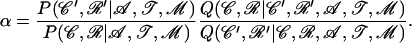
Finally, we present a reanalysis of the Bacillus data set described in Priest et al. (2004). We calculated a 95% majority-rule consensus genealogy assuming no recombination (Figure 4A) and estimating recombination parameters and location of imports from the data (Figure 4B), on the basis of 100,000 iterations including 50,000 burn-in iterations, which required ∼6 hr on a desktop computer. This consensus was highly replicable between different runs of the algorithm. Figure 4D shows the location of imports for each of the seven MLST loci estimated for a selection of branches as indicated in Figure 4B.

Figure 4.—

Application to MLST data of Bacillus. (A) The output of our program with R fixed at 0; (B) the output of our program with R inferred; (C) the eBURST output. Each row of D corresponds to the inferred events on a branch of B as labeled. The columns correspond to the seven housekeeping gene fragments of the Bacillus MLST scheme. Black crosses indicate inferred substitutions with the intensity proportional to its probability and the height of the red lines represents the inferred probability for recombination on a scale from 0 to 1.

Our analysis shows that although many of the clades can be correctly identified using phylogenetic methods, ignoring recombination has important effects on the inference. First, our analysis indicates that a majority of the polymorphisms have been introduced by recombination, so that estimates of the time since divergence between lineages would be substantially overestimated by assuming a molecular clock calibrated using the mutation rate. Second, the existence of some clades is obscured by particular recombination events. For example, ST 20 is closely related to STs 58, 10, and 43, but a single genetic import in the pycA gene in the common ancestor of the latter three STs (corresponding to event G in Figure 4D) obscured this close relationship. Third, statistical support for some subdivisions, such as many of those within the Kurstaki clade, is overestimated. Indeed, the topmost node in our genealogy, indicating the relationships between Kurstaki, Cereus, and Others, is not resolved, consistent with the general difficulty in inferring deep branches when substantial recombination has taken place.

Our analysis confirms and refines the original conclusions of Priest et al. (2004), namely that some of the named groupings of Bacillus do not correspond to monophyletic groups, so that the taxonomy needs to be redefined. Our method provides the most accurate basis to date for redefining this taxonomy. The inferred value of ν is high with a 95% credibility region of 0.031–0.042 and some events have even higher values (e.g., event G in Figure 4D introduces substitutions at a rate of 0.06). Such events introduce a higher rate of polymorphism than is available in the Bacillus population studied (∼2.5–3.0%), which means that they might come from outside Bacillus. These imports have greatly increased average branch lengths, accounting for the size difference between Figure 4A and 4B. Thus, standard methods of inference assuming a coalescent model with within-population recombination would be particularly inappropriate for this data set. The average tract length of recombination chunks δ is surprisingly small with a 95% credibility region of 193–435 bp; however, this low value may in part be due to model misspecification and the fact that the gene fragments of the Bacillus MLST scheme are quite short (405 bp on average), making inference of tract size more difficult.

Our method also produces estimates of the relative frequency of recombination and mutation. However, the limited information provided by short sequence fragments and the wide variety of estimates obtained by different methods suggest that these estimates should also be treated with care. Two quite different measures have been used: the ratio of probabilities that an individual nucleotide will be altered through recombination and point mutation, r/m, and the ratio of absolute number of events ρ/θ. For Neisseria meningitidis, three quite different methods have been used to estimate r/m. Our method, using the data set of Jolley et al. (2005), which ran for 100,000 iterations including 50,000 of burn in, gives 5–8; a population genetic method based on the pattern of linkage disequilibrium within sequence fragments (McVean et al. 2002) gives 6–16; and a method based on the number of nucleotide changes within single-locus variants of robustly assigned clonal founders gives 80 (Feil et al. 1999, 2000, 2001). The three published estimates of ρ/θ are more consistent, each including 1. These are our estimate (0.7–1.2), the estimate of Jolley et al. (2005) (0.16–1.8), and that of Fraser et al. (2005) based on the distribution of allele sharing within a population (1.1). For Bacillus, 95% credibility regions for r/m and ρ/θ based on our method are 1.3–2.8 and 0.2–0.5, respectively, showing that recombination is rare compared to the level observed in Neisseria or in many other bacteria.

eBURST finds few clades in this example, reflecting a paucity of single-locus variants, implying that the STs are too distantly related to be clustered by this type of method (Figure 4C). Our method finds many more subdivisions, which is analogous to the better performance of our method for high values of θ in the simulated data. Specifically, eBURST has correctly grouped STs 25 and 8 together. Looking at the events on branches A and C on our output indicates that the difference between these two types is a single mutation on the glpF gene, making them single-locus variants of each other. However, eBURST does not see that ST 15 is also a close relative because two mutations, one on glpF and one on tpi, separate it from ST 8. A less stringent definition of clonal complexes would allow these strains to be grouped together but would not help to spot a relationship where several genes have been altered through point mutations. Examples of this are branches D, E, and F: many genes have been mutated, but in a pattern consistent with clonal evolution.

DISCUSSION

We have described a general method for using multilocus sequence data to assess the clonal relationships among a sample of bacteria. As well as defining lineages, i.e., subsets of the sample that uniquely share a particular common ancestor, the algorithm can be used to infer the relative age of each lineage, the sequence of the ancestor, and the recombination and mutation events that have taken place in giving rise to each of its descendants.

Application of our method to simulated data sets shows that as well as providing additional information that existing methods do not, our method provides more accurate subdivisions and appropriate measures of statistical uncertainty. Further, our method is uniquely able to fully and appropriately utilize information from long stretches of contiguous sequence, up to complete genomes. Although our method is slower than non-model-based approaches such as UPGMA trees or the BURST algorithm, the time taken to perform each iteration is a linear function of the product of the number N of strains and the length L of the sequences. The algorithm should be run for longer as N increases, but the algorithm remains feasible to apply to scores of bacterial genomes or MLST data from thousands of isolates.

Most problems in bacterial epidemiology and systematics require accurate information about genealogies, whether on a very short timescale (e.g., in tracking the origin of a particular disease outbreak) or on a longer one (e.g., in identifying lineages that have acquired specific phenotypes), ranging up to species splits. On short timescales, the dominant paradigm has been to identify either isolates with identical STs or “clonal complexes,” i.e., groups of closely related genotypes that share a recent common ancestor, on the basis of sharing a particular number of alleles. Over longer timescales, analysis is typically performed using phylogenetic methods, on the basis of a large number of concatenated fragments (Gevers et al. 2005). Our method allows us to estimate degrees of relatedness at a wide range of different timescales using a single unified approach. Indeed application of our method correctly indicates that sharing the same ST can provide quite different information on when the strains last shared a common ancestor, depending on the genotypes of the rest of the sample. ST complexes can also differ considerably in their antiquity. Since the method provides indications of uncertainty it also indicates when there is insufficient information to infer clonal relationships in a given data set.

An advantage of model-based approaches over ad hoc methods is that they can be refined to take into account a wide variety of features of the data. For example, instead of the Jukes–Cantor model for mutation used here, it would be possible to incorporate more sophisticated models of mutation, such as those discussed in Whelan et al. (2001). Incorporating such a parametric mutational model into our inferential framework would be straightforward. In addition to assuming a simple mutational model, our method does not take into account insertions, deletions, or rearrangements and can handle only fully aligned sequence data. In principle it might be possible to jointly infer alignment and genealogy (Suchard and Redelings 2006). The model we use for the prior on the genealogies is a standard coalescent that assumes a constant population size. This can be generalized to include population subdivisions and growth as described in Wilson et al. (2003). It would also be possible to allow changes in demographic parameters and mutation or recombination rates in different parts of the genealogy (e.g., Drummond et al. 2005, 2006).

The key assumptions of the model concern recombination. The method does not attempt to model the origin of genetic imports and instead assumes that imports introduce a uniform rate of novel substitutions ν. As a consequence, the model tends to underestimate the number of recombinations as opposed to mutation events and can infer incorrect subdivisions, particularly if recombination is frequent compared to mutation. There are a number of different ways of addressing these limitations. For example, it should be relatively easy to assign putative origins for inferred imports on the basis of homology with different sequences from within or external to the data set in question and hence to make inferences on patterns of recombination in bacteria, which can be highly nonrandom (Zhu et al. 2001; Didelot et al. 2007; Falush et al. 2006).

It might also be possible to incorporate some information on origin of imports directly into the model. For example, for each branch in the genealogy, it would be possible to distinguish between substitutions that are novel and those that are already present in another lineage. Those that are present are more likely to have been introduced by recombination and also provide information about the likely origin of the event. Another interesting refinement would be to make the substitution rate in recombined regions nonconstant. One way to do this would be to have a different value of ν for each recombined region, but this implies a nonconstant dimensionality of the parameter space, which requires the use of complex inferential methods, for example, reversible-jump MCMC (Green 1995) or exact sampling (Fearnhead 2006). Alternatives include having a different value of ν for each branch or having several possible values of ν representing different distances of the import source. Each of these refinements would make the inference a lot slower unless efficient approximations can be found.

In summary, we find that the method that we described here provides accurate estimation of bacterial genealogies and specific genetic changes both for simulated data and for real data. The application of our general approach to the large-scale DNA sequence data sets that are becoming available should facilitate a detailed understanding of patterns of microevolution and phenotypic change (Falush and Bowden 2006) in diverse bacterial genera.

The algorithms described in this article have been implemented in a computer software package, ClonalFrame, which is available at http://bacteria.stats.ox.ac.uk/.

APPENDIX A: MARKOVIAN STRUCTURE OF THE RECOMBINED AND UNRECOMBINED REGIONS

Under our model, recombination may happen several times on a branch of the tree and affect the same portion of the genome repetitively. However, because recombination erases previous polymorphism accumulated through recombination and mutation for that branch, it is impossible to tell how many successive recombination events took place. We therefore describe each site of each branch as having two states: imported or unimported. The lengths of imported and nonimported regions follow complex distributions that are, respectively, those of busy and idle periods of an M/M/∞ queue with arrival rate Rlu/2 and mean service requirement δ as studied by Roijers et al. (2007).

To facilitate statistical inference, we approximate the relationship of these two states for a branch of length l to make it Markovian with transition matrix from one nucleotide to the next equal to

(A1)

Where α(l)⁻¹ and β(l)⁻¹ are set to be equal to the means of the busy and idle periods of an M/M/∞ queue, respectively,

(A2)

Consequently, the average length of an imported region is α(l)⁻¹ and the average length of an unimported region is β(l)⁻¹.

The imported and unimported states are not observed directly for each branch but the level of polymorphism between the genotypes at the top and the bottom of a branch gives us some information on the state. Under our model, the expected polymorphism rates in affected and unaffected regions are ν and θl/2L, respectively. We can therefore use a hidden Markov model to infer the location of affected and unaffected regions given the genotype at the top and at the bottom of a branch of 𝒯.

APPENDIX B: UPDATE OF THE ANCESTRAL SEQUENCES AND MAPS OF IMPORT

We consider a nonroot node n. Let a and b denote the children of n and f denote its father. Let l_n, l_a, and l_b denote the lengths of the branches above n, a, and b, respectively. We need to update the ancestral sequence c_n and map of imports r_n of n, as well as the map of imports r_a and r_b of the two children of n given the rest of the parameters and the data. These depend only on l_n, l_a, and l_b and the ancestral sequences c_a, c_b, and c_f of a, b, and f, so that we need to sample from . To do so, we first sample from and then sample from .

To sample from , we consider the HMM (Durbin et al. 1998; Rabiner 1989), where at each location the hidden states are the values of r_n, r_a, and r_b and the observed messages are the values of c_f, c_a, and c_b. This HMM has eight different possible hidden states because r_n, r_a, and r_b take values in {0, 1} (0 for a nonimported region and 1 for an imported region) and five messages (enumerated in the emission matrix section below). Samples from are obtained using the forward–backward algorithm, with the transition and emission matrices detailed below. The second step, sampling from , is straightforward: we calculate for each position the probabilities of c_n to be A, C, G, and T given l_n, l_a, l_b, r_n, r_a, r_b, c_f, c_a, and c_b at that position and choose one of the four possibilities with their respective probabilities.

Transition matrix:

Let π_i denote the hidden state at site i and x_i denote the message at site i. The transition matrix T is defined by . Here T is simply a function of the α(l) and β(l) for the branches above and below n: each term of T is equal to the product for each j ∈ {n, a, b} of β(l_j) if r_j stays in a nonimported region, 1 − β(l_j) if r_j steps into an imported region, 1 − α(l_j) if r_j stays in an imported region, and α(l_j) if r_j steps into a nonimported region.

Emission matrix:

The emission matrix E is defined by e_s,m = P(x_i = m | π_i = s). For j ∈ {n, a, b} let μ_j = θl_j/(2L) if r_j is in a nonimported region and ν otherwise. Assuming that there are no repeat mutations on each branch, the emission probabilities in E are equal to (1 − μ_n)(1 − μ_a)(1 − μ_b) + μ_nμ_aμ_b/9 for message 1 (c_f, c_a, and c_b are equal), (1 − μ_a)(1 − μ_b)μ_n + μ_aμ_b(1 − μ_n)/3 + 2μ_nμ_aμ_b/9 for message 2 (c_f is different from c_a and c_b), (1 − μ_n)(1 − μ_b)μ_a + μ_bμ_n(1 − μ_a)/3 + 2μ_nμ_aμ_b/9 for message 3 (c_a is different from c_f and c_b), (1 − μ_n)(1 − μ_a)μ_b + μ_aμ_n(1 − μ_b)/3 + 2μ_nμ_aμ_b/9 for message 4 (c_b is different from c_f and c_a), and 2(1 − μ_n)μ_aμ_b/3 + 2(1 − μ_a)μ_nμ_b/3 + 2(1 − μ_b)μ_nμ_a/3 + 2μ_nμ_aμ_b/9 for message 5 (c_f, c_a, and c_b are all different).

Forward–backward algorithm:

We can use the transition and emission matrices T and E above to calculate the matrix F, where f_s,i = P(x₁, … , x_i, π_i = s). This is done by using the recursion equation

(B1)

We can then draw π_L from P(π_L = s) = f_s,L and each π_i iteratively for all i from L − 1 down to 1, using

(B2)

The complexity of this algorithm is O(M²L), where L is the length of the alignment and M the number of hidden states (eight here). This is acceptable even for full bacterial genomes where the length of an alignment is a few million base pairs, but as this procedure will be called repetitively in the Monte Carlo Markov chain for each internal node of the phylogeny, a considerable proportion of the time will be spent in it and it is therefore interesting to optimize it as much as possible.

Optimization:

One way in which this algorithm can be made much faster is to calculate only the values of f_s,i for a subset of the sites that we call the “reference sites.” We used the polymorphic sites, the sites at the beginning or end of blocks, and additional sites at intervals of 50 bp. If p(i) denotes the ith reference site then Equation B1 becomes

(B3)

where

(B4)

The values of Q can be calculated recursively, using

(B5)

Note that as the values of Q do not depend on p(i) and p(i + 1) but only on their difference d, Q can be calculated once and for all before applying the forward–backward algorithm for all d = [1, … , max_{i∈[1,…,L−1]}(p(i + 1) − p(i))].

In the backward step, we use the following equation instead of (B2):

(B6)

This determines the hidden states at all reference sites. To finish, we determine the hidden states between two reference sites by assuming that there is no change of state when two consecutive polymorphic sites have the same state and assuming that there is only one transition point when they are different. For a transition between states x and y at distance d from each other, the probability that the transition is at a distance i from the polymorphic site of state x for all i ∈ [0, … , d] is given by

(B7)

It is possible to verify that this approximation has only a minor effect on the behavior of the program by calculating the acceptance ratio of the move as if it was a Metropolis–Hastings move; i.e., the ratio

(B8)

As this is a Gibbs move, the acceptance ratio should be equal to one. Without the approximation above α = 1 exactly, which proves that the move is working as expected and with the approximation log(α) varies between −1 and 1, which means that this approximation does not have much effect on the behavior of the move.

APPENDIX C: UPDATE OF THE PARAMETER MODELS ℳ AND THE AGES OF THE GENEALOGY

Let ℳ denote the set of parameters of our model, i.e., . Depending on how much prior information we have on each of these parameters we might want to estimate them or not in the MCMC.

ν is the only one that can be updated using a Gibbs step: as the likelihood is a binomial function of ν, using a conjugate Beta prior for ν leads to a Beta-distributed posterior. Here we used a Beta(1, 1) prior for ν, i.e., a uniform prior on [0, 1]. A non-Beta prior distribution can also be assumed if we use a Metropolis–Hastings move as described below.

For R, δ⁻¹, and θ we have to use a Metropolis–Hastings update. A natural uninformative prior is a uniform prior for the log of each parameter. To make it proper, we consider only values of each parameter between 10⁻¹⁰ and 1.

We propose to update the value of log(θ) by adding s to it with s drawn uniformly from [−0.05; 0.05]. If the proposed value is <10⁻¹⁰ or >1, the move is rejected. This move is symmetric and its acceptance probability is simply equal to the minimum of one and the ratio of posterior probabilities calculated using Equation 5.

The ages of 𝒯 are updated using Metropolis–Hastings updates. For each internal node n of the tree 𝒯, its age is updated by adding to it a random draw from Unif([−0.05, 0.05]). If the new age is <0, less than the age of one of the children of n, or more than the age of the father of n, then the move is rejected. The proposal distribution is therefore symmetric and the move is accepted with a probability equal to the minimum of one and the ratio of the likelihood with the new age over the likelihood before the update.

APPENDIX D: DEALING WITH MISSING DATA

There can be several reasons why an alignment contains gaps. First, deletions and insertions in one sequence create indels that correspond to small gaps in the alignment. Second, when aligning genomes against each other, if one sequence is incomplete then gaps may appear in the alignment depending on which alignment method is used. Finally, sequences sometimes contain uncertainty about some of the nucleotides.

Here we treat gaps in the input alignment as missing data. Each missing nucleotide of each sequence in 𝒜 is therefore considered to be a parameter over which we need to mix as well as for any other parameter. Let 𝒢 denote the set of these missing nucleotides. We use a Gibbs step to update 𝒢 given 𝒜 and the current values of all the other parameters. Our prior for each missing nucleotide is uniform over the four possible nucleotides.

Clearly, the value of each missing nucleotide g in sequence a depends only on the value x at that position in the ancestral sequence of the father of a in 𝒯, the value r of the locations of recombinations on the branch above a, and the length l of the branch above a:

• If r = 0, g = x with probability 1 − θl/(2L) and equals something else with probability θl/(6L);

• If r = 1, g = x with probability 1 − ν and equals something else with probability ν/3.

References

- Bryant, D., 1997. Hunting for trees, building trees and comparing trees: theory and method in phylogenetic analysis. Ph.D. Thesis, Department of Mathematics, University of Canterbury, Christchurch, New Zealand.
- Darling, A. C., B. Mau, F. R. Blattner and N. T. Perna, 2004. Mauve: multiple alignment of conserved genomic sequence with rearrangements. Genome Res. 14: 1394–1403. [DOI] [PMC free article] [PubMed] [Google Scholar]
- Didelot, X., M. Achtman, J. Parkhill, N. R. Thomson and D. Falush, 2007. A bimodal pattern of relatedness between the Salmonella paratyphi A and typhi genomes: Convergence or divergence by homologous recombination? Genome Res. 17: 61–68. [DOI] [PMC free article] [PubMed] [Google Scholar]
- Dingle, K. E., F. M. Colles, D. Falush and M. C. Maiden, 2005. Sequence typing and comparison of population biology of Campylobacter coli and Campylobacter jejuni. J. Clin. Microbiol. 43: 340–347. [DOI] [PMC free article] [PubMed] [Google Scholar]
- Donnelly, P., and S. Tavaré, 1995. Coalescents and genealogical structure under neutrality. Annu. Rev. Genet. 29: 401–421. [DOI] [PubMed] [Google Scholar]
- Drummond, A., and A. Rambaut, 2003. BEAST v1.0 (http://evolve.zoo.ox.ac.uk/beast/).
- Drummond, A., A. Rambaut, B. Shapiro and O. Pybus, 2005. Bayesian coalescent inference of past population dynamics from molecular sequences. Mol. Biol. Evol. 22: 1185–1192. [DOI] [PubMed] [Google Scholar]
- Drummond, A. J., S. Y. Ho, M. J. Phillips and A. Rambaut, 2006. Relaxed phylogenetics and dating with confidence. PLoS Biol. 4: e88. [DOI] [PMC free article] [PubMed] [Google Scholar]
- Durbin, R., S. Eddy, A. Krogh and G. Mitchison, 1998. Biological Sequence Analysis: Probabilistic Models of Proteins and Nucleic Acids. Cambridge University Press, Cambridge/London/New York.
- Falush, D., and R. Bowden, 2006. Genome-wide association mapping in bacteria? Trends Microbiol. 14: 353–355. [DOI] [PubMed] [Google Scholar]
- Falush, D., M. Torpdahl, X. Didelot, D. F. Conrad, D. J. Wilson et al., 2006. Mismatch induced speciation in Salmonella: model and data. Philos. Trans. R. Soc. B 361: 2045–2053. [DOI] [PMC free article] [PubMed] [Google Scholar]
- Fearnhead, P., 2006. Exact and efficient Bayesian inference for multiple changepoint problems. Stat. Comput. 16: 203–213. [Google Scholar]
- Feil, E., M. Maiden, M. Achtman and B. Spratt, 1999. The relative contributions of recombination and mutation to the divergence of clones of Neisseria meningitidis. Mol. Biol. Evol. 16: 1496–1502. [DOI] [PubMed] [Google Scholar]
- Feil, E. J., J. M. Smith, M. C. Enright and B. G. Spratt, 2000. Estimating recombinational parameters in Streptococcus pneumoniae from multilocus sequence typing data. Genetics 154: 1439–1450. [DOI] [PMC free article] [PubMed] [Google Scholar]
- Feil, E. J., E. C. Holmes, M. C. Enright, D. E. Bessen, N. P. J. Day et al., 2001. Recombination within natural populations of pathogenic bacteria: short-term empirical estimates and long-term phylogenetic consequences. Proc. Natl. Acad. Sci. USA 98: 182–187. [DOI] [PMC free article] [PubMed] [Google Scholar]
- Feil, E. J., B. C. Li, D. M. Aanensen, W. P. Hanage and B. G. Spratt, 2004. eBURST: inferring patterns of evolutionary descent among clusters of related bacterial genotypes from multilocus sequence typing data. J. Bacteriol. 186: 1518–1530. [DOI] [PMC free article] [PubMed] [Google Scholar]
- Felsenstein, J., 1989. PHYLIP—phylogeny inference package (version 3.2). Cladistics 5: 164–166. [Google Scholar]
- Fraser, C., W. P. Hanage and B. G. Spratt, 2005. Neutral microepidemic evolution of bacterial pathogens. Proc. Natl. Acad. Sci. USA 102: 1968–1973. [DOI] [PMC free article] [PubMed] [Google Scholar]
- Gansner, E. R., and S. C. North, 2000. An open graph visualization system and its applications to software engineering. Softw. Pract. Exper. 30: 1203–1233. [Google Scholar]
- Gelman, A., and D. B. Rubin, 1992. Inference from iterative simulation using multiple sequences. Stat. Sci. 7: 457–511. [Google Scholar]
- Gevers, D., F. M. Cohan, J. G. Lawrence, B. G. Spratt, T. Coenye et al., 2005. Re-evaluating prokaryotic species. Nat. Rev. Microbiol. 3: 733–739. [DOI] [PubMed] [Google Scholar]
- Gilks, W. R., S. Richardson and D. J. Spiegelhalter, 1998. Markov Chain Monte Carlo in Practice. Chapman & Hall, London/New York.
- Green, P. J., 1995. Reversible jump Markov chain Monte Carlo computation and Bayesian model determination. Biometrika 82: 711–732. [Google Scholar]
- Griffiths, R., and P. Marjoram, 1996. Ancestral inference from samples of DNA sequences with recombination. J. Comput. Biol. 3: 479–502. [DOI] [PubMed] [Google Scholar]
- Hudson, R. R., 1983. Properties of a neutral allele model with intragenic recombination. Theor. Popul. Biol. 23: 183–201. [DOI] [PubMed] [Google Scholar]
- Jolley, K. A., E. J. Feil, M.-S. Chan and M. C. J. Maiden, 2001. Sequence type analysis and recombinational tests (START). Bioinformatics 17: 1230–1231. [DOI] [PubMed] [Google Scholar]
- Jolley, K. A., D. J. Wilson, P. Kriz, G. Mcvean and M. C. J. Maiden, 2005. The influence of mutation, recombination, population history, and selection on patterns of genetic diversity in Neisseria meningitidis. Mol. Biol. Evol. 22: 562–569. [DOI] [PubMed] [Google Scholar]
- Jukes, T. H., and C. R. Cantor, 1969. Evolution of protein molecules, pp. 21–132 in Mammalian Protein Metabolism, edited by H. N. Munro. Academic Press, New York.
- Kingman, J. F. C., 1982. The coalescent. Stoch. Proc. Appl. 13: 235–248. [Google Scholar]
- Kumar, S., K. Tamura, I. B. Jakobsen and M. Nei, 2001. MEGA2: molecular evolutionary genetics analysis software. Bioinformatics 17: 1244–1245. [DOI] [PubMed] [Google Scholar]
- Lawrence, J., and H. Hendrickson, 2003. Lateral gene transfer: When will adolescence end? Mol. Microbiol. 50: 739–749. [DOI] [PubMed] [Google Scholar]
- Maiden, M. C. J., J. A. Bygraves, E. Feil, G. Morelli, J. E. Russell et al., 1998. Multilocus sequence typing: a portable approach to the identification of clones within populations of pathogenic microorganisms. Proc. Natl. Acad. Sci. USA 95: 3140–3145. [DOI] [PMC free article] [PubMed] [Google Scholar]
- Maynard Smith, J., N. Smith, M. O'Rourke and B. Spratt, 1993. How clonal are bacteria? Proc. Natl. Acad. Sci. USA 90: 4384–4388. [DOI] [PMC free article] [PubMed] [Google Scholar]
- McClelland, M., K. E. Sanderson, J. Spieth, S. W. Clifton, P. Latreille et al., 2001. Complete genome sequence of Salmonella enterica serovar Typhimurium LT2. Nature 413: 852–856. [DOI] [PubMed] [Google Scholar]
- McVean, G. A., and N. J. Cardin, 2005. Approximating the coalescent with recombination. Philos. Trans. R. Soc. Lond. B Biol. Sci. 360: 1387–1393. [DOI] [PMC free article] [PubMed] [Google Scholar]
- McVean, G., P. Awadalla and P. Fearnhead, 2002. A coalescent-based method for detecting and estimating recombination from gene sequences. Genetics 160: 1231–1241. [DOI] [PMC free article] [PubMed] [Google Scholar]
- Milkman, R., and M. M. Bridges, 1990. Molecular evolution of the Escherichia coli chromosome. III. Clonal frames. Genetics 126: 505–517. [DOI] [PMC free article] [PubMed] [Google Scholar]
- Milkman, R., and I. Crawford, 1983. Clustered third-base substitutions among wild strains of Escherichia coli. Science 221: 378–380. [DOI] [PubMed] [Google Scholar]
- Ochman, H., J. G. Lawrence and E. A. Groisman, 2000. Lateral gene transfer and the nature of bacterial innovation. Nature 405: 299–304. [DOI] [PubMed] [Google Scholar]
- Priest, F. G., M. Barker, L. W. Baillie, E. C. Holmes and M. C. Maiden, 2004. Population structure and evolution of the Bacillus cereus group. J. Bacteriol. 186: 7959–7970. [DOI] [PMC free article] [PubMed] [Google Scholar]
- Pritchard, J., M. Stephens and P. J. Donnelly, 2000. Inference of population structure using multilocus genotype data. Genetics 155: 945–959. [DOI] [PMC free article] [PubMed] [Google Scholar]
- Rabiner, L. R., 1989. A tutorial on hidden Markov models and selected applications in speech recognition. Proc. IEEE 77: 257–286. [Google Scholar]
- Roijers, F., M. Mandjes and J. van den Berg, 2007. Analysis of congestion periods of an M/M/inf-queue. Performance Evaluation (in press).
- Schierup, M. H., and J. Hein, 2000. Consequences of recombination on traditional phylogenetic analysis. Genetics 156: 879–891. [DOI] [PMC free article] [PubMed] [Google Scholar]
- Spratt, B., W. Hanage, B. Li, D. Aanensen and E. Feil, 2004. Displaying the relatedness among isolates of bacterial species—the eBURST approach. FEMS Microbiol. Lett. 241: 129–134. [DOI] [PubMed] [Google Scholar]
- Suchard, M. A., and B. D. Redelings, 2006. BAli-Phy: simultaneous Bayesian inference of alignment and phylogeny. Bioinformatics 22: 2047–2048. [DOI] [PubMed] [Google Scholar]
- Swofford, D., 2002. PAUP*. Phylogenetic Analysis Using Parsimony (*and Other Methods), Version 4. Sinauer Associates, Sunderland, MA.
- Whelan, S., P. Li and N. Goldman, 2001. Molecular phylogenetics: state-of-the art methods for looking into the past. Trends Genet. 17: 262–272. [DOI] [PubMed] [Google Scholar]
- Wilson, I. J., and D. J. Balding, 1998. Genealogical inference from microsatellite data. Genetics 150: 499–510. [DOI] [PMC free article] [PubMed] [Google Scholar]
- Wilson, I. J., M. E. Weale and D. J. Balding, 2003. Inferences from DNA data: population histories, evolutionary processes and forensic match probabilities. J. R. Stat. Soc. Ser. A 166: 155–188. [Google Scholar]
- Zhu, P., A. van der Ende, D. Falush, N. Brieske, G. Morelli et al., 2001. Fit genotypes and escape variants of subgroup III Neisseria meningitidis during three pandemics of epidemic meningitis. Proc. Natl. Acad. Sci. USA 98: 15056–15061. [DOI] [PMC free article] [PubMed] [Google Scholar]